Slope stability prediction under seismic loading based on the EO-LightGBM algorithm

Predicting the stability of slopes under seismic conditions is critical for geological hazard prevention and infrastructure safety. This study proposes an optimized prediction model based on EO-LightGBM to enhance the accuracy of slope stability assessment. A dataset containing 96 numerical simulation cases was constructed using FLAC3D, incorporating key influencing factors such as slope angle, inclination angle, slope height, rock mechanical parameters, and hard-to-soft rock thickness ratio. The dataset was split into a training set (76 samples) and a test set (20 samples). LightGBM, a gradient boosting decision tree (GBDT) model, was initially trained on the dataset, while Equilibrium Optimizer (EO) was utilized for hyperparameter optimization, focusing on learning rate, number of decision trees, maximum depth, and number of leaf nodes. The five-fold cross-validation approach was adopted to evaluate model generalization ability. The experimental results demonstrate that EO-LightGBM achieves a prediction accuracy of 94.0%, precision of 96.0%, recall of 92.0%, and an F1-score of 96.0%, outperforming traditional machine learning models such as SVM, KNN, and Decision Tree. Comparative analysis further confirms that EO-LightGBM effectively reduces error rates and enhances the adaptability of slope stability prediction models under complex seismic conditions. This study provides a reliable computational tool for seismic slope stability evaluation, contributing to improved risk assessment in geotechnical engineering.

1 Introduction

Seismic slope stability assessment is of great significance in the fields of geological engineering and infrastructure safety (Ahangari Nanehkaran et al., 2022; Mahmoodzadeh et al., 2022; Zeng et al., 2021). Slope instability induced by earthquakes may lead may lead to severe economic losses and casualties. Similarly, cyclic loading in subsurface environments, such as that around buried cables, alters material properties over time, making accurate prediction of slope stability under seismic loading a critical aspect of disaster prevention and mitigation (Qin and Chian, 2018; Qin and Zhou, 2023). Traditional slope stability analysis methods primarily include the Limit Equilibrium Method (LEM) and various computational tools, as seen across disciplines from fluid dynamics to geotechnical engineering (Deng et al., 2017), Lattice Element Methods (LEM) have proven effective in capturing multiphysics interactions in geomaterials, offering an alternative to traditional FEM/DEM approaches (Xu et al., 2020). (Azarafza et al., 2021) investigated the application of the limit equilibrium method in discontinuous rock slope stability analysis and found that this method is widely applicable under various failure mechanisms and geological conditions due to its computational simplicity, short analysis time, and compatibility with probabilistic statistical approaches for assessing safety factors and potential sliding surfaces. Additionally, the study summarized two-dimensional and three-dimensional slope stability analysis methods based on the limit equilibrium approach and explored its application prospects in natural slopes and artificial cut slopes. Kalatehjari and Ali (2013) examined the instability factors of slopes along a highway in Anhui, China, and discovered risks of wedge failure and toppling instability due to jointed rock layers and discontinuities. The study employed DIP.6 for kinematic analysis and Slide 6.020 for limit equilibrium analysis to determine slope instability conditions. The results indicated that empirical methods combined with limit equilibrium analysis effectively validate slope failure mechanisms and provide a basis for slope reinforcement design. The limit equilibrium method evaluates slope stability by assuming sliding surfaces and calculating mechanical equilibrium but does not account for the nonlinear deformation characteristics of materials or the cyclic response of geomaterials under repeated loading conditions (Deng et al., 2017). Su and Shao (2021) proposed a three-dimensional slope stability analysis method based on finite element stress analysis, demonstrating its capability to compute both local and overall safety factors for sliding surfaces. The study introduced an improved ellipsoidal sliding surface construction method to enhance critical surface search accuracy and employed a two-stage particle swarm optimization algorithm to optimize the sliding surface search. The results showed that this method effectively computes safety factors for non-spherical sliding surfaces and exhibits high consistency with the strength reduction method, verifying its applicability and effectiveness. Kardani et al. (2021a) developed a hybrid stacked ensemble approach combining finite element analysis (FEA) and field data to enhance slope stability prediction accuracy. The study utilized the Artificial Bee Colony (ABC) algorithm to optimize the combination of base classifiers and selected an appropriate first-level meta-classifier from 11 optimized machine learning (OML) algorithms. Finite element analysis generated synthetic databases for model training, while real-world slope cases were used for model testing. Finite element analysis can simulate slope deformation and stress distribution under seismic loading but has a high computational cost. Sun et al. (2022) proposed a novel approach (Y-slope) to simulate the entire slope failure process, including failure initiation, propagation, and deposition. This algorithm integrates finite element and discrete element methods and improves computational efficiency by incorporating absorbing boundary conditions to balance the initial stress state. The study adopted the strength reduction method, considering both tensile and shear failure modes, and automatically extracted safety factors and critical failure surfaces. By introducing an energy dissipation mechanism, the model effectively simulates the kinematic process of slope blocks in the later failure stages. Numerical tests validated the accuracy and robustness of Y-slope, demonstrating the failure mechanisms and processes of homogeneous and jointed rock slopes. Mebrahtu et al. (2022) investigated the deep-seated landslides in the Debre Sina region of Ethiopia and found that landslides frequently occur in this area. The study assessed the stability of complex slopes composed of different geological materials using the limit equilibrium method and the shear strength reduction method based on finite element analysis. The results indicated that slopes exhibited instability under both static and pseudo-static loading conditions, with stability strongly influenced by saturation conditions and seismic loads. Although the discrete element method is suitable for simulating large deformations and failure processes, obtaining high-precision input parameters in practical applications remains challenging. Furthermore, the computational accuracy of these methods largely depends on empirical parameter selection, making them less adaptable for slope stability assessment under complex working conditions.

With the advancement of artificial intelligence (AI) and machine learning (ML) technologies, data-driven approaches have been widely applied in slope stability prediction. Zhang et al. (2022) developed a support vector machine (SVM)-based slope stability prediction model and proposed an algorithm for handling complex data. The study first established an SVM regression model and optimized its parameters using a grid search. The model was trained on slope datasets, and the optimized SVM prediction results were compared with those of random forests and artificial neural networks. Lin et al. (2024) investigated a convolutional neural network with self-attention (CNN-SA)-based multi-material slope stability prediction model and proposed an integrated prediction approach applicable to soil, rock, and soil-rock mixed slopes. The study utilized digital twin (DT) technology to construct a small-scale numerical slope dataset, adjusting parameters to create a dataset containing 19,666 slope scenarios. A total of 80% of the data was used to train the CNN-SA model, while the remaining 20% and six real-world slopes were used for testing. Xie et al. (2022) proposed a random forest (RF)-based rock slope angle prediction model using real-world measurement data. The study selected ten key factors affecting slope angles, including rock strength, rock quality designation (RQD), joint spacing, continuity, aperture, roughness, filling, weathering, groundwater, and engineering direction, as independent variables to construct an RF prediction model. Machine learning methods such as support vector machines (SVM), decision trees (DT), random forests (RF), and gradient boosting decision trees (GBDT) have been applied to slope stability prediction. These methods learn complex nonlinear relationships from large-scale datasets, including those combining analytical and machine learning techniques for thermal and geomechanical property estimation (Rizvi et al., 2020a). Kai and Ke (2022) developed a LightGBM-based slope stability prediction model to mitigate slope failure-induced disasters and accidents. The study selected six key factors—unit weight, cohesion, internal friction angle, slope angle, slope height, and pore water pressure ratio—as input variables, with slope stability as the output variable. The model’s generalization ability was evaluated using a confusion matrix and AUC. The results demonstrated that LightGBM effectively captures the nonlinear relationships between influencing factors and slope stability. Light Gradient Boosting Machine (LightGBM), as an efficient algorithm based on gradient boosting decision trees, has gained widespread attention in engineering geology due to its fast computation speed, superir model performance, and suitability for large-scale datasets. To address recent advancements in machine learning applications for slope stability prediction and to highlight the novelty of our proposed approach, a summary of representative studies is provided in Table 1. Although LightGBM has demonstrated promising performance in slope stability prediction, and related numerical techniques such as lattice element modeling have been successfully used to characterize soil behavior, its effectiveness is highly dependent on appropriate hyperparameter tuning (Rizvi et al., 2018). As summarized in Table 1, various machine learning-based models, including hybrid frameworks combining metaheuristics and classical ML algorithms, have been explored to enhance prediction accuracy. These studies highlight different optimization strategies, data requirements, and performance metrics. However, they also reveal certain limitations, such as reliance on synthetic datasets, lack of cross-domain generalization, or insufficient integration with engineering knowledge. Therefore, to address these gaps, this study proposes an EO-LightGBM model that leverages the global optimization capability of the Equilibrium Optimizer (EO) to improve hyperparameter selection, thereby enhancing the model’s robustness and predictive performance for slope stability analysis under seismic conditions. Key hyperparameters such as learning rate, number of trees, maximum depth, and number of leaves have different optimal combinations across datasets. Traditional hyperparameter optimization methods like Grid Search and Random Search have low computational efficiency in high-dimensional parameter spaces and may converge to local optima.

Table 1

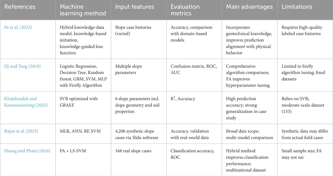
Table 1. Summary of representative studies on slope stability prediction using machine learning methods.

To address this issue, metaheuristic optimization algorithms such as Genetic Algorithm (GA), Particle Swarm Optimization (PSO), and Differential Evolution (DE) have been introduced to optimize hyperparameters globally and enhance model predictive capabilities. Among these, the Equilibrium Optimizer (EO) has gained increasing attention. EO, proposed by Afshin Faramarzi et al., in 2020, is inspired by the mass balance phenomenon and performs global search through equilibrium state simulation. Sun et al. (2023) explored an EO-LightGBM model for inverse analysis of mechanical parameters of surrounding rock in soft rock tunnels. The study used displacement data for inversion analysis and validated the results through FLAC3D numerical simulations, achieving a maximum mean error of 6.03%, demonstrating the rationality and accuracy of the EO-LightGBM model. EO simulates mass transfer between different equilibrium states to optimize variables toward optimal solutions, thereby improving search efficiency and global convergence. Compared to other optimization algorithms, EO has fewer control parameters and benefits from integration with advanced modeling techniques such as dynamic lattice element simulations of cemented geomaterials (Rizvi et al., 2020b). Previous studies have shown that EO effectively enhances classification and regression tasks by optimizing machine learning model hyperparameters. This study integrates EO with LightGBM to develop an EO-LightGBM model for hyperparameter optimization and improved slope stability prediction accuracy. The FLAC3D numerical simulation software is used to construct a seismic slope stability dataset, generating 96 slope stability cases with different slope angles, inclinations, heights, rock mechanical parameters, and soft-to-hard rock thickness ratios. The dataset consists of 76 samples for model training and 20 samples for testing. LightGBM is initially trained, and EO is used to optimize hyperparameters to enhance prediction performance. Five-fold cross-validation is employed to ensure model generalization and reduce bias from data partitioning.

2 Methods

2.1 Equilibrium optimizer algorithm (EO)

The Equilibrium Optimizer (EO) algorithm was proposed by Afshin Faramarzi et al., in 2020, with the fundamental idea of performing a global optimization search by simulating the mass balance phenomenon (Wang et al., 2021; Micev et al., 2021; Kardani et al., 2021b). The EO algorithm is designed based on the mass balance equation within a control volume, enabling efficient searching within the solution space while avoiding local optima. The search process of EO is established on a mathematical model that guides optimization variables toward the target equilibrium state. Assuming the optimization problem aims to minimize an objective function, as shown in Equation 1.

$\min f\left(X\right),X\in \mathrm{\Omega }(1)$

where X = [x1,x2, ,xn] represents a candidate solution in the search space, and Ω denotes the feasible solution domain. EO introduces multiple equilibrium state solutions X_eq, which represent the optimal solutions that may be reached during the search process. The equilibrium state solutions are computed based on historical best solutions and updated using statistical information from the search population, defined as as shown in Equation 2.

${\mathbf{X}}_{eq}=\frac{1}{N}{\displaystyle \sum _{i=1}^N}{w}_i·{\mathbf{X}}_i(2)$

where N represents the number of equilibrium state solutions, w_i is the weight coefficient, and Xi denotes the best solution selected from the current population.

The core of the algorithm is updating the solution position based on the mass balance equation. EO establishes an optimization model based on equilibrium states, assuming that the update process of solution Xt at iteration t satisfies as shown in Equation 3.

${\mathbf{X}}_{t+1}={\mathbf{X}}_{eq}+r_1\left({\mathbf{X}}_{eq}-{\mathbf{X}}_t\right)+r_2·F(3)$

where r₁ and r₂ are random numbers controlling the search step size and direction, and F is the search factor, defined as shown in Equation 4.

$F=\lambda ·\left(UB-LB\right)·r_3(4)$

where λ is the control parameter, UB and LB are the upper and lower bounds of the variables, respectively, and r₃ is a random perturbation factor that enhances search diversity (Wang et al., 2021). The weight is calculated using a fitness ranking method to ensure more stable optimization searching, determined as shown in Equation 5.

$w_i=\frac{f\left(X_i\right)-f\left(X_{\text{best}}\right)}{{\displaystyle {\sum }_{j-1}^N}\left(f\left(X_j\right)-f\left(X_{\text{best}}\right)\right)}(5)$

where f(X_best) represents the optimal fitness value in the current population. A balance factor G is introduced to regulate the search intensity, as shown in Equation 6.

$G=G_0{e}^{-\frac{t}{T}}(6)$

where G₀ is the initial balance factor, T is the maximum number of iterations, and t is the current iteration count. The optimization process typically terminates at the maximum iteration count T or when the convergence condition is met, as shown in Equation 7.

$\left|f\left(X_t\right)-f\left(X_{t-1}\right)\right|<ϵ(7)$

where ϵ is the convergence threshold, indicating that the variation in the objective function has become sufficiently small.

2.2 LightGBM ensemble learning

LightGBM (Light Gradient Boosting Machine) is an efficient machine learning algorithm based on Gradient Boosting Decision Trees (GBDT), which achieves powerful ensemble learning capabilities through the gradient boosting framework (Guo et al., 2023; Sai et al., 2023). LightGBM employs a histogram-based method for decision tree splitting and improves computational efficiency and prediction accuracy using a leaf-wise growth strategy.

LightGBM is built upon the GBDT method, with the core idea of iteratively training multiple weak learners, where each new model fits the residuals of the previous iteration, allowing the overall model to gradually converge to the optimal solution. Given a dataset $\mathcal{D}={\left\{\left(x_i,y_i\right)\right\}}_{i-1}^N$, where x_i represents the input features and yi denotes the true labels, GBDT optimizes the objective function iteratively, as shown in Equation 8.

$F_t\left(x\right)=F_{t-1}\left(x\right)+\eta h_t\left(x\right)(8)$

where F_t(x) represents the cumulative prediction model at the tth iteration, h_t(x) is the weak learner (regression tree) trained in the tth iteration, and η is the learning rate that controls the update magnitude of the model. In each iteration, GBDT computes the gradient direction based on the objective loss function and fits the negative gradient using a new regression tree, as shown in Equation 9.

$h_t\left(x\right)=\arg \underset{h}{\min }{\displaystyle \sum _{i=1}^N}L\left(y_i,F_{t-1}\left(x_i\right)+h\left(x_i\right)\right)(9)$

where $L\left(y_i,F\left(x_i\right)\right)$ represents the loss function, and the commonly used squared loss function $L{\left(y,F\left(x\right))=(y-F\left(x\right)\right)}^2$ is used to compute the prediction error. LightGBM improves upon traditional GBDT by optimizing splitting strategies and training methods, including histogram-based splitting, efficient data storage, leaf-wise growth strategies, and categorical feature processing.

LightGBM employs a histogram-based method for feature partitioning, discretizing continuous features into a fixed number of bins, where each bin represents a range of feature values. This approach reduces memory consumption and accelerates computation. For a given feature x, LightGBM constructs a histogram H, as shown in Equation 10.

$H_j={\displaystyle \sum _{x_i\in B_j}}{g}_i,H_j^{\prime }={\displaystyle \sum _{x_i\in B_j}}{h}_i(10)$

where g_i and h_i represent the first-order and second-order gradients of the objective loss function, respectively. Bj denotes the feature value range of the jth bin, while Hj and Hj’ represent the sum of the first-order and second-order gradients of all samples within that bin. LightGBM selects the optimal split point by computing the gain value of the histogram, as shown in Equation 11.

$\text{Gain}=\frac{{\left(H_L\right)}^2}{H_L^{\prime }}+\frac{{\left(H_R\right)}^2}{H_R^{\prime }}-\frac{{\left(H_T\right)}^2}{H_T^{\prime }}(11)$

where H_L and H_L’ represent the first-order and second-order gradients of the left child node, H_R and H_R’ denote the first-order and second-order gradients of the right child node, and H_T and H_T’ correspond to the first-order and second-order gradients of the current node. During the tree growth process, the leaf node with the highest gain is selected for splitting to ensure a more balanced tree structure, as shown in Equation 12.

$\text{SplitNode}=\arg \underset{\text{leaf}}{\max }\text{Gain}\left(\text{leaf}\right)(12)$

This strategy enables faster loss reduction, enhances the model’s representation capability, and avoids unnecessary computations. LightGBM incorporates L₁ and L₂ regularization terms into the objective function to prevent model overfitting, with the regularized objective function formulated as shown in Equation 13 (Sibindi et al., 2023).

$L\left(F\right)={\displaystyle \sum _{i=1}^N}L\left(y_i,F\left(x_i\right)\right)+{\lambda }_1‖w{\Vert }_1+{\lambda }_2‖w{\Vert }_2^2(13)$

where ${\lambda }_1‖w{\Vert }_1$ represents the L₁ regularization term, which enhances sparsity, and ${\lambda }_2‖w{\Vert }_2^2$ represents the L₂ regularization term, which prevents overly large parameters from causing model overfitting. Feature importance is determined by the number of splits, as shown in Equation 14.

$I_j={\displaystyle \sum _{t\in {\mathcal{T}}_j}}{\text{Gain}}_t(14)$

where Tj represents the set of all tree nodes where feature j is used for splitting, and Gaint denotes the gain value of the node. Ultimately, features with lower importance scores can be pruned to improve training efficiency. The training process typically terminates when one of the following conditions is met: the number of training iterations reaches the predefined maximum T, or the change in the loss function falls below the predefined threshold ϵ, as shown in Equation 15.

$\left|L_t-L_{t-1}\right|<ϵ(15)$

2.3 EO-LightGBM integrated model

The workflow of the EO-LightGBM-based seismic slope stability prediction model is illustrated in Figure 1. The dataset is generated through numerical simulations using FLAC software to ensure accuracy and diversity, covering slope stability characteristics under various working conditions. After dataset construction, the data is split into a training set (76 samples) and a test set (20 samples) in an 8:2 ratio, where the training set is used for model training, and the test set is used for performance evaluation. During the training process, the 76 training samples are first fed into the LightGBM model, where a classifier is constructed based on the Gradient Boosting Decision Tree (GBDT). Since the LightGBM model includes multiple key hyperparameters, such as learning rate, number of decision trees, maximum depth, and number of leaf nodes, the Equilibrium Optimizer (EO) is employed for hyperparameter tuning. By simulating the mass balance-based search strategy, EO optimizes hyperparameter combinations to enhance model predictive performance. A specific objective function is defined to evaluate model performance under different parameter combinations, and the EO algorithm searches within the parameter space to achieve the optimal objective function value, thereby constructing the optimized prediction model EO-LightGBM. During model training, a five-fold cross-validation method is applied to assess generalization capability. Upon training completion, the optimal model is saved and validated using the test set to evaluate its prediction accuracy for slope stability. In addition to the EO-LightGBM model, conventional models are also trained for comparative analysis. Various performance metrics, including accuracy, precision, recall, and F1-score, are computed to assess predictive performance, demonstrating the advantages of the EO-LightGBM model in seismic slope stability prediction tasks.

Figure 1

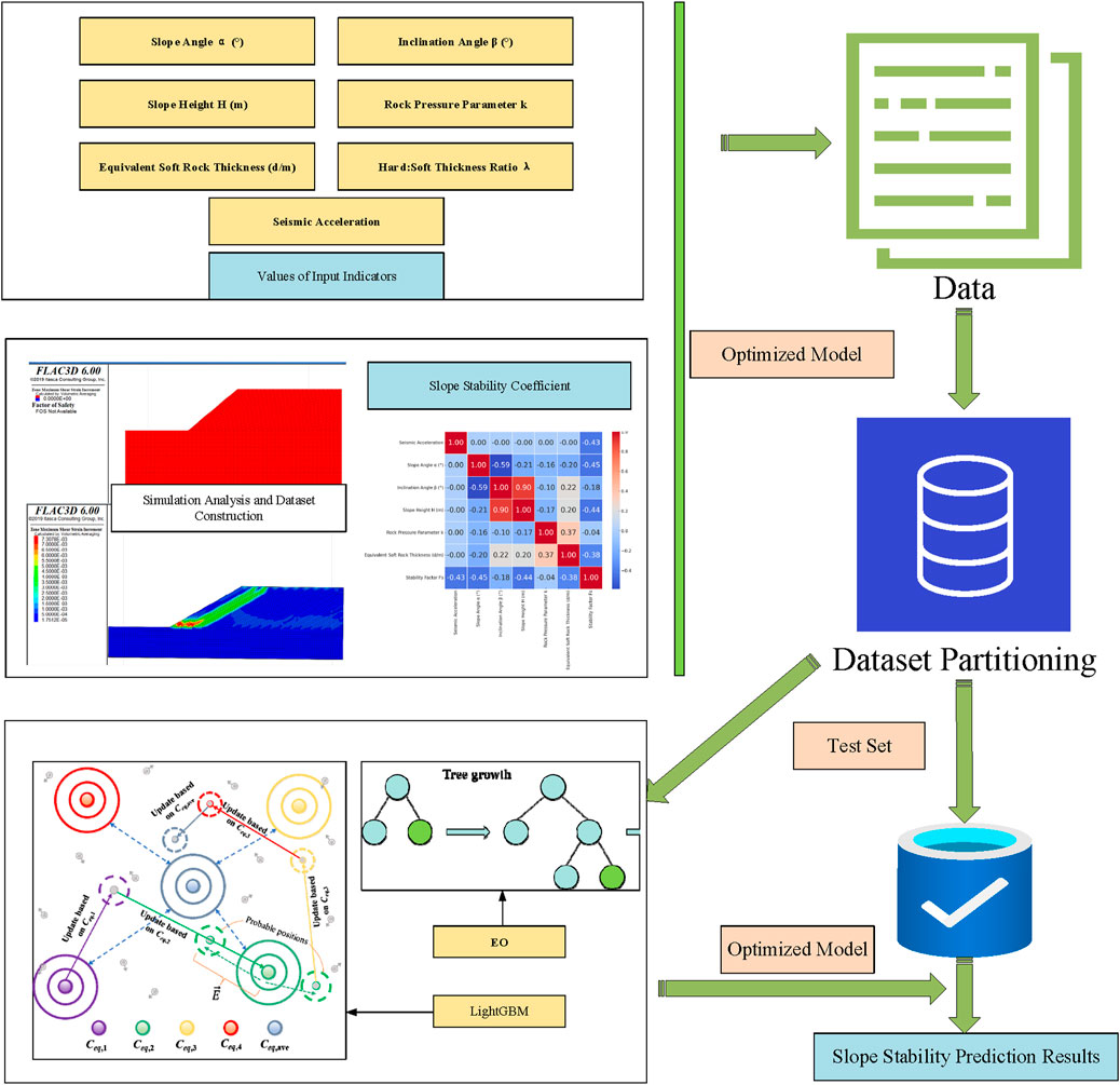
Figure 1. Slope stability prediction workflow.

In the EO-LightGBM model, the hyperparameter optimization process was implemented as follows. The search space for hyperparameters was defined within practical engineering ranges: learning rate [0.01, 0.3], number of decision trees [50, 300], maximum tree depth (Zeng et al., 2021; Zhang et al., 2022), and number of leaf nodes [10, 80]. The initial population size was set to 30, and each individual represented a set of hyperparameter combinations. The EO algorithm simulated the mass balance transfer among individuals to iteratively update solutions. Random initialization ensured population diversity. The stopping criterion was set as either reaching a maximum of 100 iterations or achieving convergence when the objective function change was less than ×110⁻⁴. During the search, five-fold cross-validation error was used as the objective function to guide the optimization. This design ensured a balanced exploration and exploitation process, enhancing the stability and reproducibility of hyperparameter selection.

3 Slope stability prediction and analysis

3.1 Dataset construction

3.1.1 Simulation model construction and experimental design

The FLAC3D software is utilized to investigate the dynamic response mechanisms of soft and hard rock slopes under seismic loading. A high-precision finite element simulation model is established to address the complex nonlinear behavior inherent in geotechnical dynamic problems. The ideal linear elastic constitutive model and the Mohr–Coulomb criterion are adopted as instability criteria to characterize the failure behavior of geomaterials under seismic excitation. Additionally, strain-softening characteristics are incorporated to simulate the influence of different lithologies on the dynamic stability of slopes (Yuan et al., 2024; Qi, 2023). To enhance computational accuracy, a high-resolution unstructured mesh is applied for model discretization, with particular emphasis on refining the mesh density along the slope surface and within critical failure zones to accurately capture stress concentration effects. The mesh configuration is illustrated in Figure 2. Seismic loading is applied using dynamic acceleration time histories with varying intensities, frequencies, and durations to replicate real seismic effects. Three representative synthetic seismic motions are selected for loading, and their corresponding time history curves are presented in Figure 3. The study primarily analyzes the dynamic response characteristics of slopes under different seismic magnitudes, lithological distributions, and slope angles, focusing on parameters such as displacement, acceleration, stress distribution, and failure modes. Seismic loading is applied through a combination of equivalent static loading and time-domain dynamic analysis methods, where the former provides a preliminary assessment of overall slope stability and the latter captures transient dynamic response characteristics. The boundary conditions incorporate a combination of free-field and non-reflective boundaries to minimize seismic wave reflections and ensure the realistic propagation of seismic loading.

Figure 2

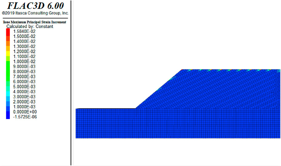
Figure 2. Example of soft and hard rock slope numerical model construction.

Figure 3

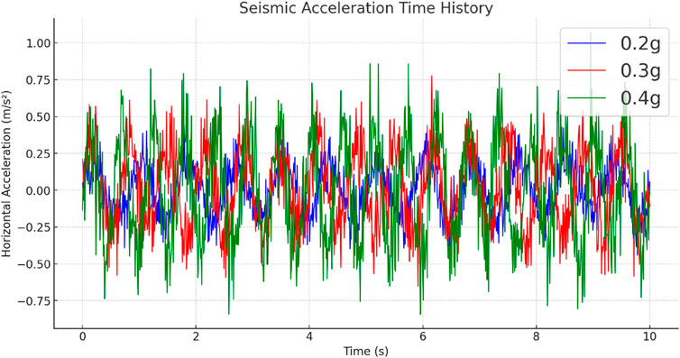
Figure 3. Artificially synthesized seismic acceleration time histories.

The experimental parameter settings are shown in Table 2. The computational results of different models will be used to evaluate the impact of soft-hard rock interfaces on the dynamic stability of slopes, revealing the Fs values of slopes under seismic loading. Table 3 presents the source code configuration for a specific experiment implemented in FLAC3D 3.0 software.

Table 2

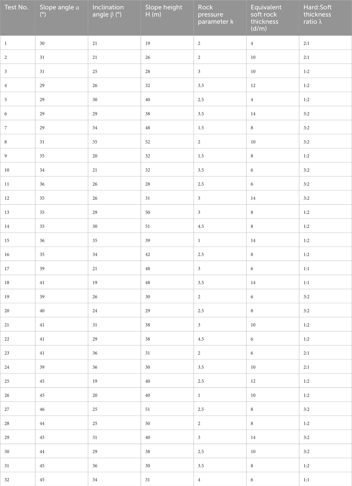
Table 2. Experimental parameters table for dynamic response of soft and hard rock slopes.

Table 3

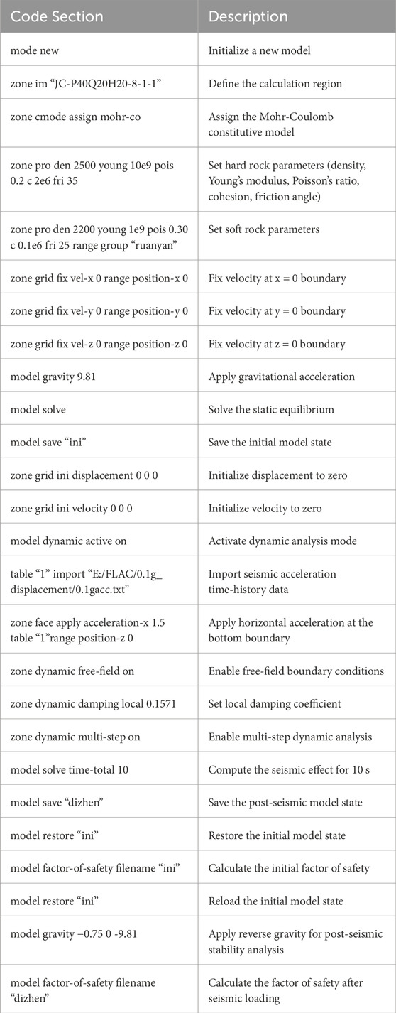
Table 3. FLAC3D simulation code example.

3.1.2 Data results and statistical analysis

In slope stability studies, statistical analysis of key parameters can reveal the primary factors influencing slope stability and provide data support for subsequent predictive model development. Geological and mechanical characteristic variables, such as seismic loading, slope angle, slope height, and rock pressure parameters, exhibit different distribution trends and correlations under various conditions. To investigate these relationships, this study employs scatter plot distribution analysis and correlation analysis to examine the distribution characteristics of the data and the interrelationships among variables. The detailed analysis results are presented in Figure 4.

Figure 4

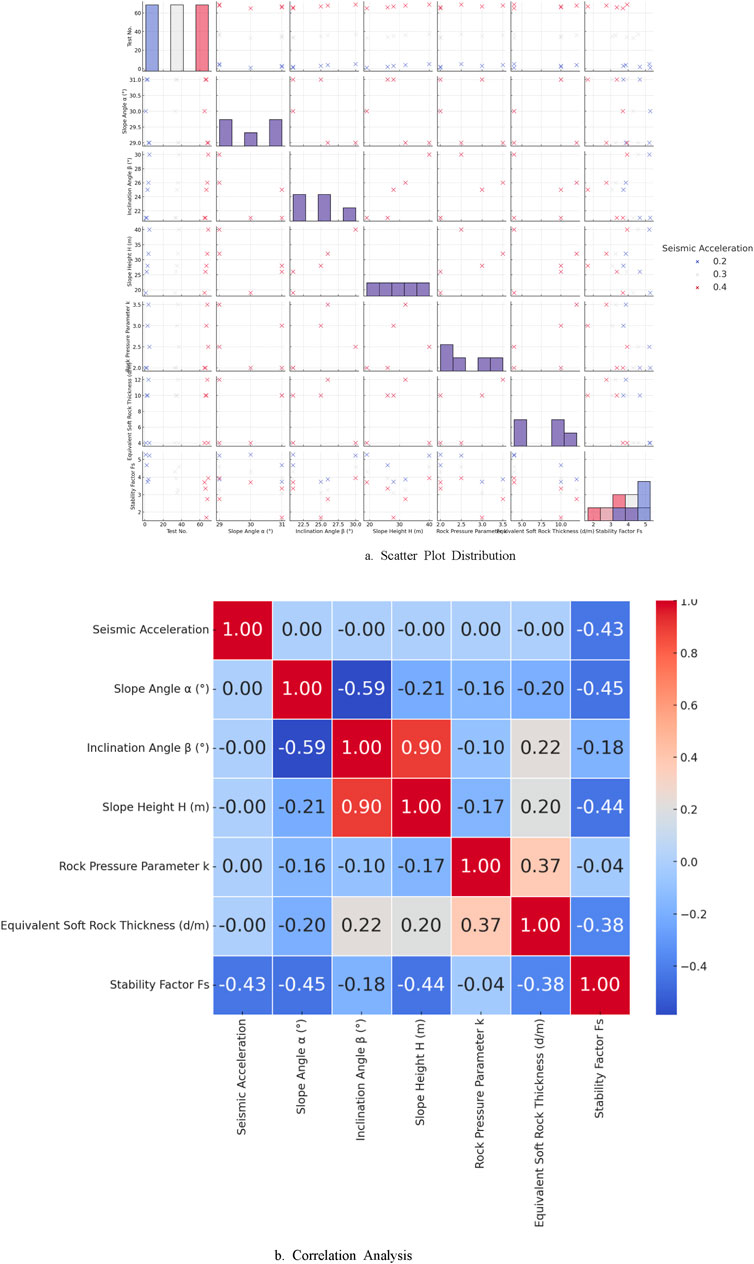
Figure 4. Statistical analysis of data. (a) Scatter plot distribution (b) correlation analysis.

Figure 4a illustrates the scatter plot distribution of the data. The distribution of samples under different seismic accelerations (0.2 g, 0.3 g, 0.4 g) across various variable spaces is visually presented, with the diagonal elements representing the histogram distribution of each variable. The scatter plot reveals that the values of slope height, slope angle, and rock pressure parameters are relatively concentrated, while the dispersion of data varies under different acceleration conditions. The Fs exhibits distinct distribution characteristics across different variables, with parameters such as slope angle and slope height having a significant influence. The overall distribution trend reflects the potential impact of different variables on slope stability. Figure 4b presents the correlation matrix heatmap, where correlation coefficients between variables are depicted using a color gradient. Positive correlations are indicated by warm colors, while negative correlations are represented by cool colors, with the intensity of the colors reflecting the strength of the correlation. The data analysis indicates that slope angle and Fs exhibit a strong negative correlation (−0.45), and slope height and Fs also show a notable negative correlation (−0.44). Additionally, seismic acceleration and Fs demonstrate a significant negative correlation (−0.43), suggesting that increasing seismic loads considerably reduce slope stability. Furthermore, the interaction between different variables, such as slope angle and slope height (−0.21), and slope angle and inclination angle (−0.59), exhibits a certain structural pattern. These correlation analysis results indicate that slope parameters and seismic loading are the key factors influencing slope stability, and the variation trends of the Fs under different variable conditions require further in-depth investigation.

To evaluate the predictive performance of the trained model, several widely used metrics are adopted, including accuracy, precision, recall, and F1-score. Accuracy reflects the overall correctness of the model’s predictions, while precision measures the proportion of true positives among all positive predictions. Recall evaluates the model’s ability to identify actual positive cases, and F1-score provides a balanced evaluation by harmonizing precision and recall. These metrics offer a comprehensive assessment of classification performance under different slope stability scenarios.

3.2 Model training and hyperparameter optimization

The EO-LightGBM algorithm is employed for model training to enhance the accuracy of slope stability prediction under seismic loading. The dataset includes key variables such as seismic acceleration, slope angle, slope height, and rock layer mechanical parameter ratios. The data is divided into a training set and a test set in an 8:2 ratio, with the training set used for model development and the test set for model evaluation. LightGBM is implemented within a gradient boosting framework that iteratively learns data features and optimizes the objective function to minimize prediction errors. Hyperparameter tuning is performed using the Equilibrium Optimizer (EO) through a global search strategy, optimizing parameters including the learning rate, number of decision trees, maximum depth, and number of leaf nodes. EO simulates the mass balance phenomenon to determine the search step size and direction, updating the hyperparameter combinations at each iteration to ensure convergence of the objective function toward an optimal value. A five-fold cross-validation approach is employed to evaluate model stability across different hyperparameter configurations, and the best parameter set is selected based on minimization of the prediction error. Figure 5 illustrates the impact of different parameter combinations on the convergence behavior of the loss function during model training.

Figure 5

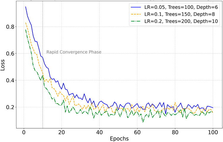
Figure 5. Loss curves for different parameter combinations after model optimization.

Figure 5 shows that all curves exhibit a rapid decline in the loss function within the initial 5–10 iterations, followed by a stabilization phase with minor fluctuations before gradually converging. When using a lower learning rate (LR = 0.05), the model experiences a smaller initial drop and a relatively slower overall convergence speed. In contrast, a higher learning rate (LR = 0.2) results in a faster decline in the loss value over the same number of iterations, maintaining the lowest level in later stages, indicating that a higher learning rate accelerates model convergence. Increasing the maximum depth and the number of decision trees further improves model convergence performance. Models with greater depth achieve lower loss values in later stages with smaller fluctuations, suggesting their superior ability to learn complex features. Overall, the parameter combination (LR = 0.2, Trees = 200, Depth = 10) exhibits the best performance in terms of loss minimization and convergence stability.

3.3 Analysis of prediction results

To validate the accuracy of the EO-LightGBM model in predicting slope stability, a total of 20 test samples were input into the trained and saved optimal predictive model for evaluation. To facilitate the prediction analysis of the slope Fs, the regression problem was transformed into a classification problem, where a slope Fs greater than 1 was classified as 1 (stable), while a factor less than 1 was classified as 0 (unstable). The prediction results of the EO-LightGBM model were compared with those of the LightGBM model alone and the actual slope stability conditions. Incorrectly predicted samples were marked with (×) in the visualization, as illustrated in Figures 6, 7.

Figure 6

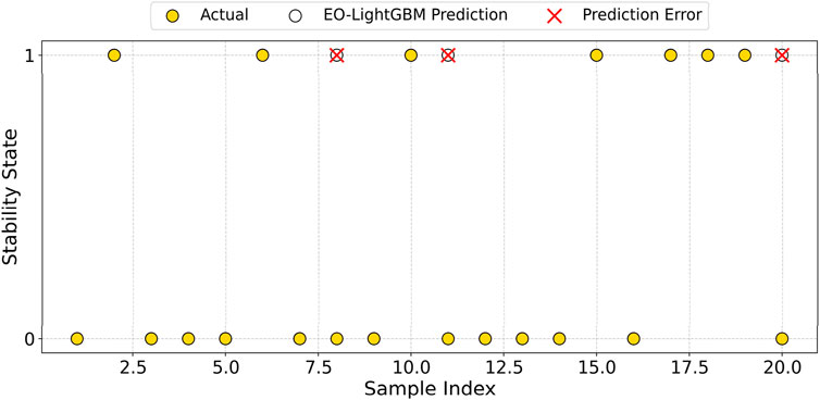
Figure 6. Comparison of EO-LightGBM predictions and actual slope stability states.

Figure 7

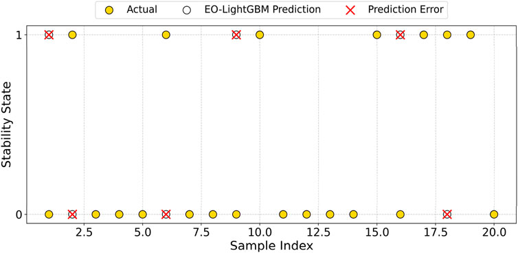
Figure 7. Comparison of LightGBM predictions and actual slope stability states.

Figure 6 presents the comparison between EO-LightGBM predictions and actual slope stability conditions. The majority of the predicted results are consistent with the actual stability states, with only a few misclassified samples. These misclassified samples are primarily located near the decision boundary, indicating that the model may still produce misclassifications under specific conditions. Overall, EO-LightGBM exhibits fewer prediction errors, and the distribution of errors is relatively scattered, demonstrating its strong generalization ability and high accuracy in identifying slope stability conditions.

Figure 7 illustrates the comparison between LightGBM predictions and actual slope stability conditions. Compared to Figure 6, the number of misclassified samples in the LightGBM model is higher, with errors more concentrated within the data distribution, particularly near the decision boundary. The increase in error rate reflects that the model’s adaptability to complex slope data is slightly inferior to that of EO-LightGBM, indicating that applying EO for hyperparameter optimization enhances prediction accuracy and reduces misclassification.Experimental results demonstrate that EO-LightGBM exhibits higher accuracy in slope stability prediction, with the optimized model significantly reducing errors and improving the model’s ability to distinguish slope stability conditions more effectively.

3.4 Comparative analysis with traditional machine learning models

To further validate the advantages of the EO-LightGBM model in slope stability prediction, multiple traditional machine learning models were selected for comparison. The predictive performance of different models on the test set was analyzed. Figure 8 presents a comparison of EO-LightGBM with traditional models across various evaluation metrics, including accuracy, precision, recall, and F1-score, quantifying the models’ predictive capability and stability.

Figure 8

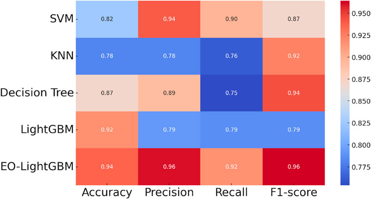
Figure 8. Comparison of prediction results with traditional models.

EO-LightGBM outperforms all compared models across all evaluation metrics, achieving an accuracy of 0.94, a precision of 0.96, a recall of 0.92, and an F1-score of 0.96, demonstrating its superiority over traditional models. Although SVM achieves a precision comparable to that of EO-LightGBM, its lower recall suggests weaker generalization capability, particularly near classification boundaries. KNN shows the weakest performance across all metrics, with a recall as low as 0.76, indicating limited capability in distinguishing between stable and unstable slope conditions. The decision tree model achieves a reasonable F1-score of 0.94 but exhibits slightly inferior stability compared to EO-LightGBM. While LightGBM performs well in terms of accuracy and precision, its overall predictive stability remains lower than that of the optimized EO-LightGBM. These results indicate that EO-LightGBM, after hyperparameter optimization, significantly enhances prediction accuracy and stability, reduces misclassification, and improves model adaptability under complex working conditions. The comparative analysis further confirms the superiority of EO-LightGBM, providing a more robust computational tool for practical applications in seismic slope stability prediction.

4 Discussion

This study constructed a dataset for the seismic stability of soft-hard interlayered rock slopes based on FLAC3D numerical simulations, and proposed an EO-LightGBM hybrid intelligent model that integrates the Equilibrium Optimizer (EO) with the Light Gradient Boosting Machine (LightGBM) to achieve efficient and high-accuracy prediction of slope safety factors under complex geological conditions. The results demonstrate that the proposed model performs well in both training and testing stages, indicating strong fitting capacity and generalization ability.

Nevertheless, there are several limitations associated with this study. First, the dataset is entirely based on numerical simulations rather than real-world monitoring data. Although simulations allow for controlled variable experiments, systematic parameter combinations, and consistent boundary conditions, they cannot fully replicate the complexity of real engineering conditions. In practice, slope stability is influenced by factors such as anisotropy of rock mass, joint distribution, fluctuations in groundwater level, and material heterogeneity, which are difficult to model comprehensively in idealized numerical simulations. This limitation may affect the model’s adaptability and robustness in real-world applications.

Second, the FLAC3D simulations adopt a linear elastic constitutive model that does not consider nonlinear deformation, strain-softening, or plastic flow behavior of rock and soil materials under strong seismic loading. As a result, the instability process in highly strained regions may not be accurately captured, potentially reducing the authenticity of the dataset used for model training. Moreover, the complex structure of soft-hard rock slopes, including weak interlayers and interface effects, has not been explicitly discussed in the simulation design or analysis.

Regarding optimization, while the Equilibrium Optimizer improves the efficiency of hyperparameter search for the LightGBM model, its performance is still constrained by initial population distribution and parameter ranges. In complex non-convex search spaces, it may fall into local optima, causing instability in training outcomes. In future studies, optimization methods such as Bayesian optimization, differential evolution, or adaptive particle swarm optimization could be introduced to enhance the reliability and convergence of hyperparameter tuning.

As for evaluation metrics, this study employed three widely used regression indicators: mean absolute error (MAE), root mean square error (RMSE), and coefficient of determination (R²). Results show that EO-LightGBM performs better than the baseline LightGBM in prediction accuracy, particularly under small-sample conditions, confirming its modeling strength in high-dimensional feature spaces. However, with only 96 samples in total, the size of the test set remains limited. Although five-fold cross-validation helps reduce evaluation bias, it cannot entirely eliminate accidental errors. Expanding the dataset and adopting Monte Carlo cross-validation would help improve the model’s robustness.

To enhance the engineering applicability and academic contribution of the proposed model, future work could proceed in the following directions:

1. Multi-source data fusion: Real monitoring data, such as InSAR displacement, fiber Bragg grating (FBG) strain measurements, and UAV-based photogrammetry, could be integrated with simulation data to improve prediction reliability under complex loading and geological conditions. Developing a comprehensive database of soft-hard rock slopes will also aid training and validation.

2. Advanced modeling strategies: Deep learning techniques such as convolutional neural networks (CNN) and long short-term memory networks (LSTM) can be introduced to extract features from spatial or spatio-temporal datasets. This is particularly valuable for handling 2D/3D data derived from images, sensors, or monitoring platforms.

3. Comparative algorithmic analysis: In addition to LightGBM, alternative models such as XGBoost, Random Forest, support vector regression (SVR), and deep neural networks (DNN) should be incorporated and compared using various metaheuristic optimizers like genetic algorithms (GA) or artificial bee colony (ABC) algorithms to comprehensively assess model effectiveness.

4. System development for practical deployment: Combining the EO-LightGBM model with a GIS-based interface can yield an intelligent slope assessment tool. Such a system can allow users to input key parameters, rapidly assess slope stability, identify high-risk zones, and generate engineering recommendations. This integration will promote intelligent design and decision-making in slope engineering.

Although the proposed EO-LightGBM model provides a promising and effective approach for seismic slope stability prediction, it must be validated on more diverse real-world cases. Future studies should focus on expanding the dataset, incorporating field data, applying advanced algorithms, and developing practical systems to improve the model’s generalization ability and engineering significance. These efforts will support disaster early warning, optimized construction practices, and intelligent slope management.

5 Conclusion

This study proposed an EO-LightGBM model for predicting slope stability under seismic loading. Based on a FLAC3D-simulated dataset of 96 samples, the model incorporates key parameters such as slope angle, height, seismic acceleration, and lithological configuration. The Equilibrium Optimizer (EO) was applied to fine-tune LightGBM hyperparameters, enhancing the model’s generalization capability and accuracy.

Experimental evaluation using five-fold cross-validation demonstrated that EO-LightGBM achieved the highest performance among all compared models. Specifically, EO-LightGBM obtained an accuracy of 0.94, precision of 0.96, recall of 0.92, and F1-score of 0.96. These metrics significantly outperformed traditional classifiers such as SVM (accuracy: 0.82, F1-score: 0.87), KNN (accuracy: 0.78, F1-score: 0.92), Decision Tree (accuracy: 0.87, F1-score: 0.94), and even non-optimized LightGBM (accuracy: 0.92, F1-score: 0.79).

The results confirm that the EO-LightGBM model provides superior predictive power and robustness, especially under complex geotechnical conditions. The hybrid strategy of combining machine learning and global optimization offers a promising approach for seismic slope stability assessment, with strong applicability in practical geohazard risk mitigation. Future work will incorporate field monitoring data and deep learning models to further enhance prediction reliability and engineering adaptability.

Data availability statement

The original contributions presented in the study are included in the article/supplementary material, further inquiries can be directed to the corresponding author.

Author contributions

NM: Conceptualization, Data curation, Formal Analysis, Funding acquisition, Investigation, Methodology, Project administration, Resources, Software, Supervision, Validation, Visualization, Writing – original draft, Writing – review and editing. YZ: Conceptualization, Data curation, Formal Analysis, Methodology, Resources, Software, Validation, Writing – original draft, Writing – review and editing. ZY: Data curation, Formal Analysis, Methodology, Project administration, Software, Validation, Visualization, Writing – original draft, Writing – review and editing.

Funding

The author(s) declare that financial support was received for the research and/or publication of this article. This work was supported by National Natural Science Foundation of China (42207192). Scientific and Technological Achievements Transformation Project of Qinghai Province (2022-SF-158). The authors also thank the editors and anonymous reviewers for their constructive comments that improved the manuscript.

Conflict of interest

The authors declare that the research was conducted in the absence of any commercial or financial relationships that could be construed as a potential conflict of interest.

Generative AI statement

The author(s) declare that no Generative AI was used in the creation of this manuscript.

Publisher’s note

All claims expressed in this article are solely those of the authors and do not necessarily represent those of their affiliated organizations, or those of the publisher, the editors and the reviewers. Any product that may be evaluated in this article, or claim that may be made by its manufacturer, is not guaranteed or endorsed by the publisher.

References

Ahangari Nanehkaran, Y., Pusatli, T., Chengyong, J., Chen, J., Cemiloglu, A., Azarafza, M., et al. (2022). Application of machine learning techniques for the estimation of the safety factor in slope stability analysis. Water 14 (22), 3743. doi:10.3390/w14223743

CrossRef Full Text | Google Scholar

Azarafza, M., Akgün, H., Ghazifard, A., Asghari-Kaljahi, E., Rahnamarad, J., and Derakhshani, R. (2021). Discontinuous rock slope stability analysis by limit equilibrium approaches–a review. Int. J. Digit. Earth 14 (12), 1918–1941. doi:10.1080/17538947.2021.1988163

CrossRef Full Text | Google Scholar

Deng, D., Li, L., and Zhao, L. (2017). Limit equilibrium method (LEM) of slope stability and calculation of comprehensive factor of safety with double strength-reduction technique. J. Mt. Sci., 14(11): 2311–2324. doi:10.1007/s11629-017-4537-2

CrossRef Full Text | Google Scholar

Guo, J., Yun, S., Meng, Y., Wang, L., Ye, D., Zhao, Z., et al. (2023). Prediction of heating and cooling loads based on light gradient boosting machine algorithms. Build. Environ. 236, 110252. doi:10.1016/j.buildenv.2023.110252

CrossRef Full Text | Google Scholar

Hoang, N. D., and Pham, A. D. (2016). Hybrid artificial intelligence approach based on metaheuristic and machine learning for slope stability assessment: a multinational data analysis. Expert Syst. Appl., 46: 60–68. doi:10.1016/j.eswa.2015.10.020

CrossRef Full Text | Google Scholar

Kai, Z., and Ke, Z. (2022). Prediction study on slope stability based on LightGBM algorithm. China Saf. Sci. J. 32 (7), 113. doi:10.16265/j.cnki.issn1003-3033.2022.07.1473

CrossRef Full Text | Google Scholar

Kalatehjari, R., and Ali, N. (2013). A review of three-dimensional slope stability analyses based on limit equilibrium method. Electron J. Geotech. Eng. 18, 119–134. Available online at https://www.researchgate.net/publication/236174492.

Google Scholar

Kardani, N., Bardhan, A., Gupta, S., Sharma, D., Chatterjee, R. S., Zhang, Y., et al. (2021b). Predicting permeability of tight carbonates using a hybrid machine learning approach of modified equilibrium optimizer and extreme learning machine. Acta Geotech. 17, 1239–1255. doi:10.1007/s11440-021-01257-y

CrossRef Full Text | Google Scholar

Kardani, N., Zhou, A., Nazem, M., Zhang, Y., and Lyu, Y. (2021a). Improved prediction of slope stability using a hybrid stacking ensemble method based on finite element analysis and field data. J. Rock Mech. Geotech. Eng. 13 (1), 188–201. doi:10.1016/j.jrmge.2020.05.011

CrossRef Full Text | Google Scholar

Khajehzadeh, M., and Keawsawasvong, S. (2023). Predicting slope safety using an optimized machine learning model. Heliyon, 9, e23012. doi:10.1016/j.heliyon.2023.e2301212).

PubMed Abstract | CrossRef Full Text | Google Scholar

Lin, M., Chen, X., Chen, G., Zhang, T., Wang, L., and Liu, Y. (2024). Stability prediction of multi-material complex slopes based on self-attention convolutional neural networks. Stoch. Environ. Res. Risk Assess., 1–17. doi:10.1007/s00477-024-02792-2

CrossRef Full Text | Google Scholar

Mahmoodzadeh, A., Mohammadi, M., Hama Ali, H. F., Ibrahim, H. H., Abdulhamid, S. N., and Nejati, H. R. (2022). Prediction of safety factors for slope stability: comparison of machine learning techniques. Nat. Hazards 111, 1771–1799. doi:10.1007/s11069-021-05115-8

CrossRef Full Text | Google Scholar

Mebrahtu, T. K., Heinze, T., Wohnlich, S., Alemayehu, T., and Dagnachew, N. (2022). Slope stability analysis of deep-seated landslides using limit equilibrium and finite element methods in Debre Sina area, Ethiopia. Bull. Eng. Geol. Environ. 81 (10), 403. doi:10.1007/s10064-022-02906-6

CrossRef Full Text | Google Scholar

Micev, M., Ćalasan, M., and Oliva, D. (2021). Design and robustness analysis of an Automatic Voltage Regulator system controller by using Equilibrium Optimizer algorithm. Comput. Electr. Eng. 89, 106930. doi:10.1016/j.compeleceng.2020.106930

CrossRef Full Text | Google Scholar

Pei, T., Qiu, T., and Shen, C. (2023). Applying knowledge-guided machine learning to slope stability prediction. J. Geotechnical Geoenvironmental Eng., 149(10): 04023089. doi:10.1061/jggefk.gteng-11053

CrossRef Full Text | Google Scholar

Qi, C., and Tang, X. (2018). Slope stability prediction using integrated metaheuristic and machine learning approaches: a comparative study. Comput. and Industrial Eng., 118: 112–122. doi:10.1016/j.cie.2018.02.028

CrossRef Full Text | Google Scholar

Qi, Y. N. (2023). FLAC3D-based slope stability analysis and calculation. Eng. Technol. 79, 22–29. doi:10.54097/hset.v79i.15075

CrossRef Full Text | Google Scholar

Qin, C., and Chian, S. C. (2018). New perspective on seismic slope stability analysis. Int. J. Geomechanics, 18(7): 06018013. doi:10.1061/(asce)gm.1943-5622.0001170

CrossRef Full Text | Google Scholar

Qin, C., and Zhou, J. (2023). On the seismic stability of soil slopes containing dual weak layers: true failure load assessment by finite-element limit-analysis. Acta Geotech. 18 (6), 3153–3175. doi:10.1007/s11440-022-01730-2

CrossRef Full Text | Google Scholar

Rajan, K. C., Aryal, M., Sharma, K., Bhandary, N. P., Pokhrel, R., Acharya, I. P., et al. (2025). Development of a framework for the prediction of slope stability using machine learning paradigms. Nat. Hazards, 121(1): 83–107. doi:10.1007/s11069-024-06819-3

CrossRef Full Text | Google Scholar

Rizvi, Z. H., Mustafa, S. H., Sattari, A. S., Ahmad, S., Furtner, P., and Wuttke, F. (2020b). “Dynamic lattice element modelling of cemented geomaterials,”IACMAG Symposium 2019: Advances in Computer Methods and Geomechanics, 1. Singapore: Springer, 655–665. doi:10.1007/978-981-15-0886-8_53

CrossRef Full Text | Google Scholar

Rizvi, Z. H., Shrestha, D., Sattari, A. S., and Ahmad, S. (2018). Numerical modelling of effective thermal conductivity for modified geomaterial using lattice element method. Heat. Mass Transf. 54, 483–499. doi:10.1007/s00231-017-2140-2

CrossRef Full Text | Google Scholar

Rizvi, Z. H., Zaidi, H. H., Akhtar, S. J., Mustafa, S. H., and Ahmad, S. (2020a). Soft and hard computation methods for estimation of the effective thermal conductivity of sands. Heat. Mass Transf. 56, 1947–1959. doi:10.1007/s00231-020-02833-w

CrossRef Full Text | Google Scholar

Sai, M. J., Chettri, P., Panigrahi, R., Nayak, J., Bhoi, A. K., and Barsocchi, P. (2023). An ensemble of Light Gradient Boosting Machine and adaptive boosting for prediction of type-2 diabetes. Int. J. Comput. Intell. Syst. 16 (1), 14. doi:10.1007/s44196-023-00184-y

CrossRef Full Text | Google Scholar

Sibindi, R., Mwangi, R. W., and Waititu, A. G. (2023). A boosting ensemble learning based hybrid light gradient boosting machine and extreme gradient boosting model for predicting house prices. Eng. Rep. 5 (4), e12599. doi:10.1002/eng2.12599

CrossRef Full Text | Google Scholar

Su, Z., and Shao, L. (2021). A three-dimensional slope stability analysis method based on finite element method stress analysis. Eng. Geol. 280, 105910. doi:10.1016/j.enggeo.2020.105910

CrossRef Full Text | Google Scholar

Sun, J., Wu, S., Wang, H., Liu, H., Tang, L., and Zhang, Y. (2023). Inversion of surrounding rock mechanical parameters in a soft rock tunnel based on a hybrid model EO-LightGBM. Rock Mech. Rock Eng. 56 (9), 6691–6707. doi:10.1007/s00603-023-03387-z

CrossRef Full Text | Google Scholar

Sun, L., Liu, Q., Abdelaziz, A., Tang, X., Wang, J., and Li, Y. (2022). Simulating the entire progressive failure process of rock slopes using the combined finite-discrete element method. Comput. Geotech. 141, 104557. doi:10.1016/j.compgeo.2021.104557

CrossRef Full Text | Google Scholar

Wang, J., Yang, B., Li, D., Zhao, Q., Chen, Y., Guo, Z., et al. (2021). Photovoltaic cell parameter estimation based on improved equilibrium optimizer algorithm. Energy Convers. Manag. 236, 114051. doi:10.1016/j.enconman.2021.114051

CrossRef Full Text | Google Scholar

Xie, H., Dong, J., Deng, Y., Liu, Y., and Zhou, Y. (2022). Prediction model of the slope angle of rocky slope stability based on random forest algorithm. Math. Probl. Eng. 2022, 9441411–10. doi:10.1155/2022/9441411

CrossRef Full Text | Google Scholar

Xu, W. J., Wang, S., and Bilal, M. (2020). LEM-DEM coupling for slope stability analysis. Sci. China Technol. Sci., 63(2): 329–340. doi:10.1007/s11431-018-9387-2

CrossRef Full Text | Google Scholar

Yuan, L., Liu, S., and Meng, L. (2024). Numerical simulation analysis of slope stability from rainwater utilizing the Civil3D + Flac3D coupling. Desalin Water Treat. 319, 100517. doi:10.1016/j.dwt.2024.100517

CrossRef Full Text | Google Scholar

Zeng, F., Nait Amar, M., Mohammed, A. S., Motahari, M. R., and Hasanipanah, M. (2021). Improving the performance of LSSVM model in predicting the safety factor for circular failure slope through optimization algorithms. Eng. Comput. 38, 1755–1766. doi:10.1007/s00366-021-01374-y

CrossRef Full Text | Google Scholar

Zhang, Y., Ming, F., and Chang, M. (2022). “A prediction model for slope stability based on the support vector machine,” in Proceedings of the 2022 international conference on computer engineering and artificial intelligence (ICCEAI) (IEEE), 41–45. doi:10.1109/ICCEAI56860.2022.00018

CrossRef Full Text | Google Scholar