Future variation and uncertainty source decomposition in deep learning bias-corrected CMIP6 global extreme precipitation historical simulation

Global circulation models (GCMs) serve as pivotal tools in climate science research. Despite their critical role in understanding and predicting climate change, GCMs often exhibit significant discrepancies with observational data due to systematic and random errors, which has driven the progress of bias correction (BC) techniques. This study explores a bias correction approach based on convolutional neural networks (CNNs) to improve the accuracy of Expert Team on Climate Change Detection and Indices (ETCCDI) extreme precipitation indices calculated from the Coupled Model Intercomparison Project Phase Six (CMIP6) daily predictions. Specifically, this research employs historical period data (1950–2014) for eight ETCCDI extreme precipitation indices from 10 GCMs to train eight individual CNN-based bias correction models, using the HadEX3 reference dataset for evaluation. All corrected data showing mean absolute percentage error (MAPE) were consistently reduced to below 0.1. Subsequently, these well-trained models are further utilized to predict ETCCDI extreme precipitation for the future under four Shared Socioeconomic Pathway (SSP) scenarios, and the projections of extreme precipitation changes are investigated across global continents. In addition, this study endeavors to separate and quantify three different components of uncertainty (model uncertainty, scenario uncertainty, and internal variability) associated with ETCCDI extreme precipitation indices and evaluate the impact of bias correction on uncertainty variation. The results indicate that CNNs are effective in correcting historical precipitation extremes. In the future period, extreme precipitation shows an increasing trend in general. The degree of change in R10mm is relatively small and reaches its peak in the medium term, whereas the variation in Rx1day is more pronounced and increases over time. Further analysis reveals that model uncertainty is the predominant source of uncertainty in ETCCDI extreme precipitation indices, accounting for more than 80% of total uncertainty. Implementation of CNNs as a BC method could significantly reduce model uncertainty but at the cost of increasing the proportion of scenario uncertainty and internal variability. This research not only highlights the potential of the CNN-based deep learning technique in enhancing the accuracy and reliability of extreme precipitation predictions but also provides insights into uncertainty decomposition and variation to better understand various sources of uncertainty within climate projections.

Highlights

1. Convolutional neural networks (CNNs) could effectively correct biases in CMIP6 extreme precipitation predictions.

2. R10mm shows minor changes and peaks in the mid-term future, whereas Rx1day consistently increases over time.

3. Model uncertainty accounts for more than 80% of total extreme precipitation prediction uncertainty.

4. The reduction of model uncertainty with CNN-based bias correction comes at the cost of increased scenario uncertainty and internal variability.

1 Introduction

Extreme climate events often lead to significant social and economic losses, especially in vulnerable countries (Otto et al., 2015). In recent decades, anthropogenic climate warming has increased atmospheric moisture content and intensified the hydrological cycle, creating conditions conducive to heavy and extreme precipitation events (de Medeiros et al., 2022). Global circulation models (GCMs) are widely recognized as effective tools for climate prediction and research (Parsons, 2020). Given the large number of GCMs worldwide, the World Climate Research Program (WCRP) coordinates international intercomparison projects known as Coupled Model Intercomparison Projects (CMIPs) to standardize and compare these models’ outputs (Dufresne et al., 2013). Recently, the IPCC released CMIP6 simulation datasets, which improve spatial resolution and physical parameterization and include additional earth system processes, such as nutrient limitations on the ice sheet dynamics and terrestrial carbon cycle (Eyring et al., 2016). However, CMIP6 outputs are subject to uncertainty, with potentially greater variations across future scenarios (Liu and Merwade, 2018; Liu et al., 2021; Liu et al., 2023). Uncertainties in climate projections primarily arise from three sources: first, model uncertainty, which arises from the incompleteness of parameterization schemes for atmospheric moist convection and cloud processes in GCMs, leading to differences in predictions among various models (Song and Zhang, 2009; Zhang and Song, 2010; Oueslati and Bellon, 2013; Deng et al., 2016; Cao and Zhang, 2017; Peters et al., 2017; Song and Zhang, 2018); second, scenario uncertainty, caused by the uncertainties in radiative forcing under different future socioeconomic pathways (Hawkins and Sutton, 2009); and third, internal variability, referring to natural fluctuations in the absence of external radiative forcing (Marotzke and Forster, 2015). It is, therefore, essential to evaluate the accuracy of CMIP6 predictions in representing extreme events and decompose the associated uncertainties to understand their variation and impact on the model predictions in both historical and future periods.

Considering the profound impact of extreme weather on human activities and safety, the Expert Team on Climate Change Detection and Indices (ETCCDI) was established by the World Meteorological Organization (WMO) and the World Climate Research Program (WCRP). These indices focus on standardizing methodologies to quantify the frequency, intensity, and duration of extreme weather and climate events. This standardization facilitates comparisons among different models across regions and time periods (Zhang et al., 2011). Statistical analysis of ETCCDI extreme precipitation indices using CMIP6 daily precipitation simulations could help reveal trends in extreme climatic events in the context of global change and assess their impact on socio-economic activities. Nevertheless, significant uncertainties exist in climate predictions due to the inherent systematic and stochastic model errors in GCMs, which lead to significant discrepancies between model outputs and actual observations (Wu et al., 2021; Kharin et al., 2013; Tebaldi et al., 2021). In recent years, numerous bias correction (BC) methods, such as quantile mapping, delta change, and machine learning-based approaches, have been developed to adjust biases in original GCM outputs (Wu et al., 2022; Maurer and Pierce, 2014). However, research on the investigation and decomposition of uncertainty for extreme precipitation and figuring out proper bias correction techniques remains limited, making it a key research hot spot in climate science (Wu et al., 2022; Maurer et al., 2016; Sangelantoni et al., 2019). With the advancement in deep learning technology and its growing application in hydrometeorological studies, these methods present promising new alternatives for correcting extreme precipitation bias (Huang et al., 2024; Huang et al., 2023).

In this study, we first assess the performance of eight ETCCDI extreme precipitation indices calculated from 10 CMIP6 models’ historical predictions with HadEX3 datasets as references. Then, the convolutional neural network-based deep learning model is employed for extreme precipitation index bias correction and the well-trained CNN models are further applied to predict eight extreme precipitation indices under four distinct Shared Socioeconomic Pathway (SSP) scenarios for the future period. Finally, we decompose the sources of uncertainty in CMIP6 future ETCCDI projections and quantify the relative contribution of each uncertainty source. In addition, we examine and compare the changes in uncertainty components before and after bias correction. Specifically, the objectives of this study are to

(1) Assess the effectiveness of CNNs in correcting historical extreme precipitation indices.

(2) Investigate the spatiotemporal variations in bias-corrected extreme precipitation indices across global continents under different future scenarios.

(3) Decompose the sources of uncertainty in future extreme precipitation projections and examine the impacts of bias correction on changes in uncertainty components.

2 Study area and data

2.1 Study area

The global land surface (excluding Antarctica) is divided into six parts, each distinguished by unique geographic and climatic features. They are named based on the location of each continent and its abbreviation (as shown in Figure 1): Asia (ASI) is known for its complex climate types, ranging from tropical monsoon to temperate continental and highland mountain climates. Africa (AFR), on the other hand, has a predominantly tropical climate, including tropical rainforest, savannah, and tropical desert climates, along with areas of Mediterranean climate. Europe and Siberia (ERU) has a mild and humid climate, with a temperate oceanic climate, a Mediterranean climate, and a predominantly temperate continental climate, especially the subarctic coniferous forest climate. North America (NAM) has a variety of climates, ranging from tropical to temperate and polar. The climate of South America (SAM) is predominantly tropical, with tropical rainforests dominating the Amazon Basin in particular. The climate of Australia (AUS) is semi-annular, with a humid east and an arid interior. The various climate types of the continents make them ideal test beds for this study.

Figure 1

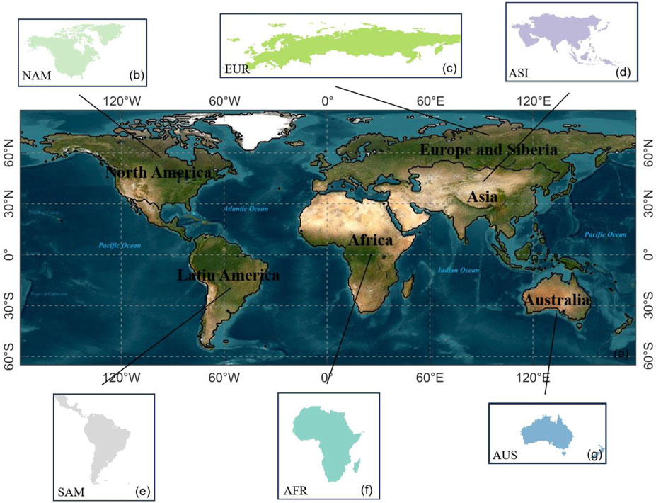
Figure 1. Layout map of six regions for this study. Globe (a), North America (b), Europe and Siberia (c), Asia (d), Latin America (e), Africa (f), and Australia (g).

2.2 Data

2.2.1 CMIP6 climate data

In this study, the daily precipitation data from 10 CMIP6 models (see Table 1; data can be downloaded from https://aims2.llnl.gov/search/cmip6) are used to calculate eight ETCCDI extreme precipitation indices, including the maximum length of a dry spell, the maximum number of consecutive days with precipitation < 1 mm (CDD), the maximum length of a wet spell, the maximum number of consecutive days with precipitation ≥1 mm (CWD), the annual total precipitation in wet days (PRCPTOT), the annual count of days when precipitation ≥10 mm (R10mm), the annual count of days when precipitation ≥20 mm (R20mm), the monthly maximum 1-day precipitation (Rx1day), the monthly maximum consecutive 5-day precipitation (Rx5day), and the simple precipitation intensity index (SDII). The simulation of the historical period is from 1950 to 2014, and the projection of the future period is from 2015 to 2100. Four Shared Socioeconomic Pathway scenarios (SSP1-2.6, SSP2-4.5, SSP3-7.0, and SSP5-8.5) representing different emission, population, economic, and social structure situations are applied in this study. All the data are regridded to 1° × 1° grids by bilinear interpolation prior to analysis. The future projections are divided into three periods in this study: 2020–2026 is defined as the near term, 2060–2066 is the medium term, and 2090–2096 is the long term. The historical period of 1970–1999 is chosen as the baseline period.

Table 1

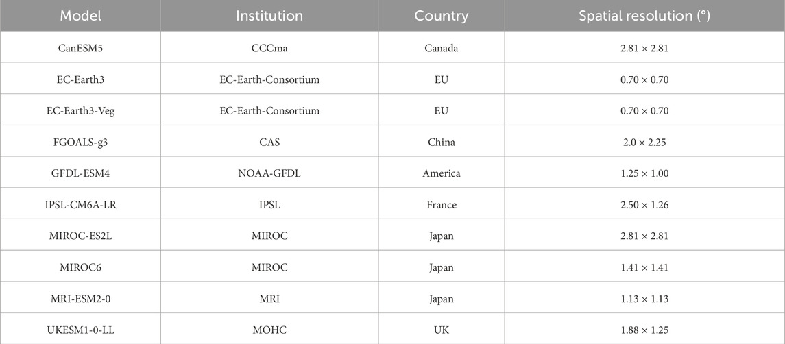
Table 1. List of 10 CMIP6 models used in this study and their original resolutions.

2.2.2 HadEX3 historical climate reference

HadEX3 is the third version of a global gridded dataset providing information on climate extremes (Dunn and Alexander, 2020; Babaousmail et al., 2021; Wang et al., 2021; Wu et al., 2021). This dataset is developed by the Climatic Research Unit (CRU) at the University of East Anglia in collaboration with other institutions. HadEX3 contains a variety of indices related to temperature and precipitation extremes, such as heat waves, cold spells, heavy rainfall events, and dry spells. Considering its extensive spatial coverage and long-term records, HadEX3 data are used as the reference dataset for this study. To facilitate the analysis and evaluation process, the bilinear interpolation technique is also used to resample the HadEX3 reference data into a 1° × 1° resolution.

3 Methodology

3.1 Expert Team on Climate Change Detection and Indices

In this study, eight extreme precipitation indices are utilized, as shown in Table 2. These eight extreme precipitation indices can be categorized into four types: absolute indices (the maximum precipitation in a year), threshold indices (the number of days with precipitation exceeding or falling below a fixed value), duration indices (the longest spell of consecutive days with precipitation exceeding or falling below a fixed value), and relative indices (the ratio of total precipitation to the number of wet days).

Table 2

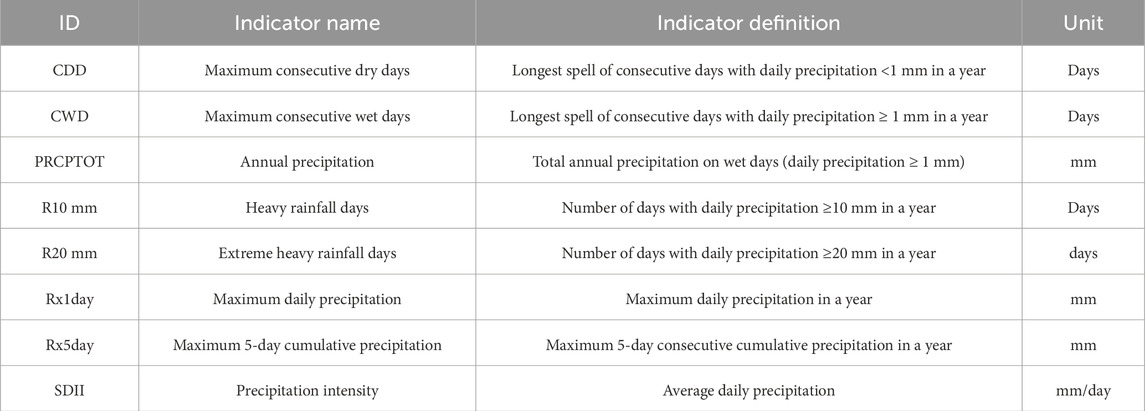
Table 2. Definitions of the extremes indices recommended by the ETCCDI.

3.2 Bias correction with convolutional neural networks

CNN is one of the most emblematic network architectures in deep learning (Guo Q et al., 2024). Compared to other deep learning methods, CNN exhibits superior capabilities in feature extraction and information mining. The working principle of CNN is shown in Figure 2. The key components of a CNN network consist of three parts, namely, the convolutional layer, the pooling layer, and the fully connected layer. The convolutional layer is mainly responsible for extracting features from the input data. Within the convolutional layer, a set of defined convolutional kernels performs convolutional operations on the input data to produce a series of feature maps. This convolution operation can effectively capture local features and spatial structure information, thus achieving effective feature extraction and representation of the input data. The role of the pooling layer is to perform downsampling on the feature maps generated by the convolution layer to reduce the number of parameters and computational complexity of the model. Commonly used pooling techniques include maximum and average pooling, which compress data by selecting the maximum or average value within a region. In this study, we employ average pooling for its superior performance with climate data: it preserves broad-scale patterns (e.g., long-term trends) while reducing noise impact, thus enhancing extreme event modeling. Its gradient-balancing improves training stability, and replacing fully-connected layers reduces overfitting. These properties make it ideal for climate analysis that requires noise robustness and regional context integration, thus justifying our choice of average pooling. In addition, pooling operations also enhance the robustness of the model to changes in position and translation, which, in turn, improve the generalization performance of the model. The fully connected layer is typically located at the end of the convolutional neural network, and its role is to integrate the features extracted from the previous convolutional and pooling layers. In the fully connected layer, each neuron is connected to all the neurons in the previous layer to achieve advanced feature learning tasks on the input data by learning weights and bias parameters. In the training process, two convolutional layers are configured. The first convolutional layer utilizes kernels of size 3 × 1 to generate 16 feature maps, whereas the second convolutional layer employs kernels of the same size of 3 × 1 to further produce 32 feature maps.

Figure 2

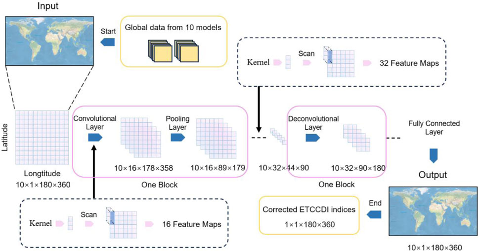
Figure 2. Schematic plot of the convolutional neural network.

The implemented CNN architecture consists of two neural layers utilizing ReLU activation functions for nonlinear feature extraction. The model employs the Adam optimizer for adaptive learning rate optimization and uses mean squared error (MSE) as the loss function for regression-oriented optimization. Training parameters were carefully configured with a learning rate of 0.01 and a batch size of 100 samples per iteration, and the model was trained for 800 complete epochs to ensure convergence while maintaining computational efficiency. This configuration balances training stability through the moderate learning rate with efficient resource utilization via the substantial batch size, while the 800-epoch duration provides sufficient training iterations for parameter optimization.

3.3 Model uncertainty decomposition

Uncertainty reflects the differences between the model’s historical simulation and the references (Wu et al., 2022). This study uses the method introduced by Hawkins and Sutton (2009) and Hawkins and Sutton (2011) in the uncertainty decomposition for R10mm and Rx1day data for future periods. These two indices are chosen because the value of R10mm serves as the representative threshold indices, whereas Rx1day represents the absolute indices, which are suitable for providing useful insights. The combined analysis of both indices provides a more comprehensive representation. The uncertainty sources are divided into three components: internal variability (I), model uncertainty (M), and scenario uncertainty (S). Internal variability refers to natural fluctuations within the climate system driven by chaotic dynamics; model uncertainty arises from structural differences, parameterizations, or incomplete physical representations across climate models; and scenario uncertainty is linked to future socioeconomic pathways and emission scenarios that depend on human choices and policy trajectories. These distinctions are essential for systematically quantifying uncertainties in climate projections. Prior to the decomposition of uncertainty, the data are processed using the 10-year moving average, which attenuates noise and reduces the effect of variation between data series (Seneviratne and Hauser, 2020). We fit the simulations of 10 CMIP6 models under the four emission scenarios from 2015 to 2100 using a fourth-order polynomial ordinary least squares method (Wu et al., 2022).

The raw simulation results for each model m, scenario s, and year t are presented in Equation 1 as follows:

$X_{m,s,t}=x_{m,s,t}+{\epsilon }_{m,s,t}.(1)$

Here, $x_{m,s,t}$ denotes the value obtained from the fourth-order fit; ${\epsilon }_{m,s,t}$ signifies the residuals from this fitted equation.

Scenario uncertainty (S, Equation 2) is defined as the variance of the mean of the 10 models under four SSP-RCP scenarios:

$S={var}_s\left(\frac{1}{N_m}{\displaystyle \sum _m}{x}_{m,s,t}\right),(2)$

where $N_m$ is the number of models.

The internal variability (V, Equation 3) of each model is considered the variance of the fitted residuals:

$V=\frac{1}{N_m}{\displaystyle \sum _m}{var}_{s,t}\left({\epsilon }_{m,s,t}\right),(3)$

where ${var}_{s,t}\left({\epsilon }_{m,s,t}\right)$ denotes the variance of model m over all scenarios and time and $N_m$ is the number of models. V remains constant over time and is independent of emission scenarios.

The model uncertainty (M, Equation 4) for a given scenario is defined as the variance between the different models in this scenario:

$M=\frac{1}{N_s}{\displaystyle \sum _s}{var}_m\left(x_{m,s,t}\right),(4)$

where $N_s$ is the number of scenarios.

We assume that there are no interactive effects among uncertainties from different sources. Therefore, the total uncertainty (T, Equation 5) can be simply regarded as the sum of uncertainties from these three independent sources:

$T=V+M+S.(5)$

The average prediction of all the models is obtained by averaging across multiple scenarios and models (Equation 6):

$G=\frac{1}{N_s}\frac{1}{N_m}{\displaystyle \sum _{m,s}}{x}_{m,s,t}.(6)$

Following the approach of Hawkins and Sutton (2009), the fractional uncertainty of a variable is defined as the ratio of predictive uncertainty to the mean prediction. This ratio helps eliminate differences between geographic regions to some extent. For example, even though temperature predictions in equatorial and polar regions may have the same level of uncertainty, the significant differences in average temperatures between these regions result in different patterns of fractional uncertainty. Fractional uncertainty (F, Equation 7) at the 90% confidence level can be expressed as follows:

$F=\frac{1.65\sqrt{T}}{G},(7)$

where 1.65 is the coefficient corresponding to the 90% confidence interval of a normal distribution. It should be noted that all models are given equal weights in this analysis. Proportional variances are represented by V/T, M/T, and S/T, which reflect the proportion of each source’s contribution to the total uncertainty.

3.4 Performance measures

In this study, the data are divided into the training period (1950–2001, 80% of the total data) and validation period (2002–2014, 20% of the total data), and multiple evaluation metrics, including mean absolute percentage error (MAPE), root mean square error (RMSE), R², mean absolute error (MAE), and mean bias error (MBE), are applied in both training and validation periods to compare the ETCCDI extreme precipitation indices calculated from 10 CMIP6 models and HadEX3 references. The details of the five metrics are shown below.

3.4.1 Mean absolute percentage error

MAPE (Equation 8) assesses the accuracy of a prediction by calculating the absolute value of the prediction error as a proportion of the true value.

$MAPE=\frac{1}{n}{\displaystyle \sum _{t=1}^n}\left|\frac{A_t-F_t}{A_t}\right|\times 100\%,(8)$

where $A_t$ is the actual value (true value) at moment t, $F_t$ is the predicted value at moment t, and n is the number of observations.

This formula represents the average of the absolute percentage of prediction error at each observation. It is important to note that if some actual value $A_t$ is 0, the denominator of this formula will be 0, which will result in uncertain or infinite MAPE. Therefore, it is necessary to ensure that all actual values are non-zero or the data are pre-processed to avoid this. In this study, linear interpolation is employed to estimate the values by averaging the data points from adjacent grid cells. In addition, one of the disadvantages of MAPE is that it is very sensitive to small values of actual observations, i.e., when the actual values are close to 0, the value of MAPE may become very large even if the prediction error is small. Therefore, the use of other evaluation metrics may need to be considered in some cases.

3.4.2 Root mean square error

RMSE (Equation 9) is a statistic used to measure the difference between the predicted and actual values, and it is often used, especially in regression analyses. RMSE can provide the absolute magnitude of the prediction error.

$RMSE=\sqrt{\frac{1}{n}{\displaystyle \sum _{i=1}^n}{\left(y_i-{\widehat{y}}_i\right)}^2},(9)$

where n is the number of samples, $y_i$ is the actual value of the ith sample, and ${\widehat{y}}_i$ is the predicted value for the ith sample.

RMSE ranges from 0 to positive infinity. A lower RMSE value (closer to 0) indicates a smaller discrepancy between the model’s predicted values and the actual observations, signifying better predictive performance. Ideally, an RMSE value of 0 signifies perfect prediction with no error. However, in practical applications, achieving perfect prediction (RMSE equals 0) is nearly impossible due to various factors such as noise and limitations in model complexity.

3.4.3 Mean absolute error

MAE (Equation 10) calculates the average of the absolute values of the prediction errors, thereby assigning equal weight to all types of errors.

$MAE=\frac{1}{n}{\displaystyle \sum _{t=1}^n}\left|A_t-F_t\right|,(10)$

where $A_t$ is the actual value (true value) at moment t, $F_t$ is the predicted value at moment t, and n is the number of observations.

3.4.4 Mean bias error

MBE (Equation 11) helps evaluate whether the prediction model exhibits a consistent bias, i.e., whether the predicted values are generally higher or lower than the actual values.

$MBE=\frac{1}{n}{\displaystyle \sum _{t=1}^n}\left(F_t-A_t\right),(11)$

where $A_t$ is the actual value (true value) at moment t, $F_t$ is the predicted value at moment t, and n is the number of observations. A positive value of MBE indicates that the predicted values are generally higher than the actual values; a negative value of MBE indicates that the predicted values are generally lower than the actual values; and an MBE close to 0 indicates that there is no significant systematic deviation between the predicted and actual values.

4 Results and discussion

4.1 Performance of CNNs in correcting bias in CMIP6 extreme precipitation indices

Figure 3 shows the performance measures of eight extreme precipitation indices, namely, CDD, CWD, PRCPTOT, R10mm, R20mm, Rx1day, Rx5day, and SDII, before and after bias correction. The results demonstrate substantial improvements across four key evaluation metrics for CNN-corrected extreme precipitation indices: the corrected MAPE, RMSE, MAE, and MBE exhibit convergence toward 0, indicating effective elimination of systematic biases. This verifies the superior capability of deep learning algorithms in modeling complex nonlinear relationships inherent in climate systems. Additionally, validation period metrics slightly diverged from training results, suggesting robust generalizability with minor overfitting risks.

Figure 3

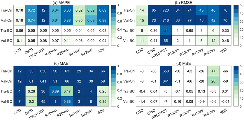
Figure 3. Performance of MAPE, RMSE, MAE, and MBE for eight ETCCDI indices (CDD, CWD, PRCPTOT, R10mm, Rx1day, Rx5day, and SDII) during 1950–2014 (training period: 1950–2001; validation period: 2002–2014) before and after bias correction with the CNN. Tra-Ori represents original data for the training period before bias correction, and Val-Ori represents original data for the validation period before bias correction. Tra-BC represents bias-corrected data for the training period, and Val-BC represents bias-corrected data for the validation period. (a–d) show the values for four performance measures mentioned in the methodology section respectively.

4.2 Variation in ETCCDI extreme precipitation indices for global continents under different future SSP-RCP scenarios

In this study, the multi-year mean extreme precipitation indices of the baseline period are subtracted from those of the near-, medium-, and long-future periods under four scenarios, respectively, to investigate the spatial variations in extreme precipitation. Specifically, we select Rx1day and R10mm indices as representative indices for further analysis due to their unique and complementary capacities in characterizing extreme precipitation features. R10mm quantifies the frequency of moderate-intensity precipitation events (annual count of days with ≥10 mm precipitation), directly reflecting persistent shifts in regional precipitation regimes. Rx1day, in contrast, captures the peak intensity of extreme precipitation (annual maximum daily precipitation), characterizing the destructive potential of short-duration deluges and flooding. Figure 4 indicates that the Rx1day index exhibits an overall increasing trend across all near, medium, and long future periods. The extreme precipitation becomes heavier from relatively mild SSP scenarios to severe SSP scenarios. In contrast, the change in the R10mm index behaves slightly differently. The overall variation in R10mm index values is relatively smaller. Although R10mm also increases globally from mild to severe SSP scenarios, it peaks in the mid-term and decreases slightly less in the long term.

Figure 4

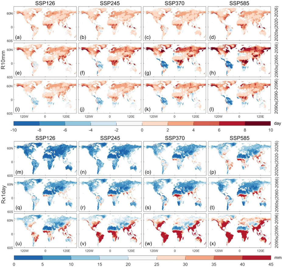
Figure 4. Projected change in R10mm and Rx1day over global continents under four SSP scenarios (SSP1-2.6, SSP2-4.5, SSP3-7.0, and SSP5-8.5) for the near- (2020–2026; a–d and m–p), medium- (2060–2066; e–h and q–t), and long-term (2090–2096; i–l and u–x) future relative to the historical baseline period (1970–1999) with CNN bias correction.

Figure 4 also indicates that Rx1day is highly sensitivity to SSP scenarios, with its variations closely aligned with SSPs and demonstrating a positive correlation over time. Notably, the magnitude of change in Rx1day is relatively small in high-latitude regions, showing significant increases only under high-emission scenarios and in the long-term future period. In contrast, the increase in Rx1day is more pronounced in low-latitude regions, indicating a greater impact of changes in Rx1day in these areas. A pronounced increase in Rx1day at low latitudes can suggest strengthened convective activity in those regions under future scenarios. Comparatively, there is a slight increase in R10mm globally for the near term for all SSP scenarios, with changes being particularly evident in low-latitude regions. During the mid-term, the rate of increase in R10mm accelerates in the Northern Hemisphere, whereas in some regions in the Southern Hemisphere, it increases very slightly or even decreases. Nevertheless, both the increasing and decreasing trends become more stable in the long-term future.

4.3 Change in different uncertainty sources associated with ETCCDI extreme precipitation projections

Fractional uncertainty refers to the ratio or fraction of the uncertainty relative to the measurement value. It can be used to express the relative error in the measurement result. Figure 5 shows that model uncertainty represents the dominant source of uncertainty, which consistently exceeds 0.15 for R10mm and 0.27 for Rx1day prior to bias correction. Model uncertainty becomes higher as it reaches the peak at 0.16 for R10mm and at 0.3 for Rx1day till the end of mid-term (approximately in 2060), after which it gradually decreases. Scenario uncertainty is the second-largest source of uncertainty and increases slowly over time. Internal uncertainty is very small compared to model uncertainty and scenario uncertainty before CNN bias correction.

Figure 5

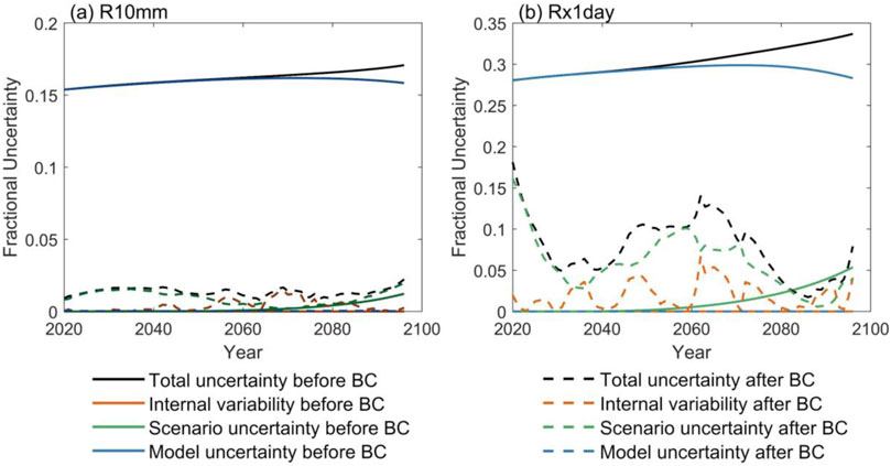
Figure 5. Fractional uncertainties of different sources in the inter-decadal CMIP6 model mean projections of (a) R10mm and (b) Rx1day for the global continents (except Antarctica).

After bias correction, the model uncertainty significantly decreases for both R10mm and Rx1day. Although there is a slight increase in the variability of uncertainty for R10mm, the magnitude of the increase is very little. In addition, neither scenario uncertainty nor internal variability shows substantial growth. However, comparatively, both scenario uncertainty and internal uncertainty increase considerably and exhibit significant variability for Rx1day after bias correction. Specifically, internal uncertainty fluctuates over time, reaching a peak of 0.0661 in 2060, whereas scenario uncertainty initially decreases and subsequently peaks at 0.1009 in 2060. Thus, bias correction with the CNN network effectively reduces model uncertainty with minimal impact on scenario uncertainty and internal variability for R10mm. Conversely, scenario uncertainty becomes the predominant and most significant source of uncertainty, followed by internal uncertainty for Rx1day after correction. Overall, the level of uncertainty is notably reduced compared to pre-correction levels, and the mid-term serves as a critical timepoint for changes in uncertainty.

It needs to be noted that the scenario uncertainty and internal uncertainty of Rx1day are significantly larger than those of the R10mm metric. This indicates that Rx1day is more sensitive to changes in future SSP scenarios and exhibits greater variability than R10mm. The implementation of bias correction can notably reduce the discrepancies in predictions among models, thereby decreasing model uncertainty. However, this approach also exacerbates the divergence in prediction results across different scenarios, leading to an increase in scenario uncertainty. Bias correction may also disrupt the inherent regularity of the original model predictions, elevating the noise level in model outputs, which, in turn, increases internal uncertainty. Furthermore, bias correction enhances the fluctuation of both internal and scenario uncertainties over time.

Figure 6 illustrates the proportions of uncertainty components across the six geographical regions through the end of this century. It is evident that model uncertainty constitutes a significant portion of the total uncertainty within all six designated regions, with the proportion showing a gradual decreasing trend over time. Australia represents an exception to this pattern. The second-largest source of uncertainty is scenario uncertainty for R10mm and internal variability for Rx1day for the future period. In contrast to the smooth transition of uncertainty in the remaining five regions, Australia experiences pronounced fluctuations over time, indicating a higher level of noise. Given the frequent occurrence of extreme climate events in Australia in recent years, along with the continent’s relatively small size and its being surrounded by oceans, these factors contribute to high uncertainties in precipitation patterns (Katelaris, 2021; Papalexiou and Montanari, 2019). Consequently, the R10mm and Rx1day indices, which are related to precipitation, exhibit higher uncertainties in the Australian (AUS) region, manifesting as pronounced variability in time-series analysis.

Figure 6

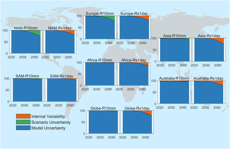
Figure 6. Proportions and variance of different uncertainty sources in decadal mean projection of ETCCDI extreme precipitation indices for R10mm (left) and Rx1day (right) over the global continents (unit: %; NAM, North America; SAM, South America).

Figure 7 shows that the spatial distributions of model uncertainty for R10mm and Rx1day exhibit generally similar patterns across near-term, mid-term, and long-term projections. Given the difficulty in obtaining precipitation data in high-elevation regions, uncertainty in such areas (such as the Tibetan Plateau) is large. For mid-high latitude regions (such as central North America, Europe, and central Siberia), climate uncertainty is influenced by a combination of geographical locations, topographical characteristics, atmospheric circulation patterns, and oceanic influences. Central North America has the extensive Great Plains, which lack significant topographical barriers, allowing cold and warm air masses to interact freely. This results in substantial temperature fluctuations and exacerbates climatic uncertainty. In contrast, Europe and central Siberia exhibit pronounced continental climate features with significant temperature differences between summer and winter due to their inland positions that are distant from maritime influences. Although these regions contain some mountain ranges, most of the landscape consists of plains or basins, which facilitates the accumulation and dispersion of cold air. Additionally, global warming has significant impacts on Siberia, including the melting of snow and ice and the thawing of permafrost, which further disrupt local climate systems and increase climatic uncertainty. Therefore, the discrepancies in climate projections among various models within these regions contribute to increased model uncertainty. Regarding the scenario uncertainties and internal variabilities of both indices, the areas characterized by higher values show slight difference from those where model uncertainties are more pronounced. The increasing trend of scenario uncertainty changes in a relatively regular manner, whereas the internal variability exhibits notable increase during the mid-term. This indicates that there is considerable internal fluctuation in the projected values of each model during this period.

Figure 7

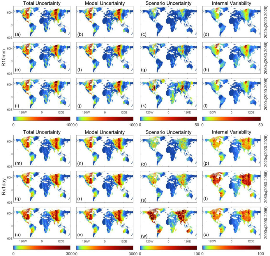
Figure 7. Uncertainty from different sources in the decadal mean projections for R10mm and Rx1day over global continents. The figure shows the near term (2020s; a–d and m–p), medium term (2060s; e–h and q–t), and long term (2090s; i–l and u–x). This graph shows four columns of uncertainty: total uncertainty (first column), model uncertainty (second column), scenario uncertainty (third column), and internal variability (fourth column).

Figure 8 illustrates the comparison of uncertainty contributions before and after bias correction for global continents. Prior to bias correction, model uncertainty is the dominant source of uncertainty for both indices: R10mm and Rx1day. The average contribution of model uncertainty for R10mm and Rx1day across near-term, mid-term, and long-term periods reached 98.5% and 92.5%, respectively. In contrast, scenario uncertainty plays a relatively minor role in the early stages but increases toward the long term, and internal uncertainty is very small for both indices. After bias correction with a CNN-based deep learning network, there is a significant reduction in model uncertainty for both indices, with scenario uncertainty exhibiting more dynamic behavior over time. Specifically, the contribution of scenario uncertainty decreased over time for the R10mm index, accompanied by an increase in the contribution from internal variability. Scenario uncertainty increases from the near term to the mid-term for Rx1day but decreases from the mid-term to the long term, indicating that the mid-term serves as a critical juncture for changes in uncertainty dynamics. Figures 5–8 demonstrate that bias correction using the CNN could effectively reduce the overall uncertainty by mitigating dominant model uncertainty. However, this process may lead to an unavoidable increase in scenario uncertainty and internal variability, enhancing their temporal variability. Nonetheless, the extent of this increase is moderate and follows a discernible pattern for different ETCCDI extreme precipitation indices. Overall, CNN-based bias correction represents an effective strategy for reducing uncertainties in climate predictions.

Figure 8

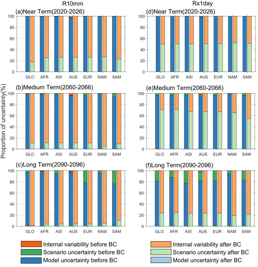
Figure 8. Proportion of uncertainty for three different sources in the decadal mean projections for R10mm (a–c) and Rx1day (d–f) before and after bias correction (BC) over global continents (unit: %). Internal variability, scenario uncertainty, and model uncertainty are represented in orange, green, and blue, respectively. The darker colors show the results before BC, and the lighter colors show the results after BC. The results shown in this figure use the CNN as the BC method. The horizontal axis of each subplot: Globe (GLO), Africa (AFR), Asia (ASI), Australia (AUS), Europe and Siberia (EUR), North America (NAM), and South America (SAM).

5 Conclusion

In this study, we utilize the CNN deep learning BC approach to correct eight ETCCDI extreme precipitation indices calculated from 10 CMIP6 models with HadEX3 references in the historical period. The well-trained CNN structure is further applied for future projections, and the variation in two representative extreme precipitation indices (Rx1day and R10mm) across global continents is evaluated and compared with the baseline period. In addition, three sources of uncertainty associated with the predictions of ETCCDI, including model uncertainty, scenario uncertainty, and internal variability, are decomposed and assessed. Specifically, the following conclusions are drawn:

1. CNN exhibits great capability for reducing model uncertainty through bias correction. The eight ETCCDI extreme precipitation indices from 10 CMIP6 models exhibited satisfactory alignment with reference datasets during training and validation periods after undergoing bias correction via CNN. This finding assures the feasibility of employing CNNs for bias correction for future projections.

2. The spatial distribution analysis of uncertainty sources for the indices Rx1day and R10mm revealed that irrespective of whether it is model uncertainty, scenario uncertainty, or internal variability, the magnitudes tend to be larger in high-altitude regions and mid-to-high latitude continental interiors (such as central North America, Europe, and central Siberia). Temporally, model uncertainty remains relatively invariant. Conversely, scenario uncertainty increases for future periods, whereas internal variability reaches its peak in the mid-term future.

3. Compared to the raw ETCCDI extreme precipitation indices calculated from CMIP6 models, CNNs can effectively reduce R10mm model uncertainty by 98.40% and Rx1day model uncertainty by 92.47% on average over a long term. However, the CNN method tends to reduce model uncertainty at the cost of simultaneously increasing the proportion of internal and scenario uncertainties.

4. Analysis of the spatiotemporal distribution of R10mm and Rx1day indicates that the increase in R10mm is most pronounced and exhibits higher sensitivity to different scenario models during the mid-term future period. As for Rx1day, it shows a monotonically increasing trend with the enhancement of the scenario and the progression of time. The uncertainty characteristics observed in the Australian region are primarily attributed to its unique geographical conditions, which have further exacerbated the region’s volatility in extreme precipitation.

Data availability statement

The raw data supporting the conclusions of this article will be made available by the authors, without undue reservation.

Author contributions

XX: Writing – original draft, Formal Analysis, Methodology, Conceptualization. YL: Formal Analysis, Writing – original draft, Conceptualization. XW: Writing – review and editing, Funding acquisition, Supervision. ZL: Funding acquisition, Writing – original draft, Conceptualization, Supervision. LW: Data curation, Writing – review and editing. BW: Data curation, Writing – review and editing. CJ: Writing – review and editing, Data curation. ZZ: Writing – review and editing, Data curation.

Funding

The author(s) declare that financial support was received for the research and/or publication of this article. This study was supported by the National Key R&D Program of China (2024YFC3211400), the National Natural Science Foundation of China (42401146), the Natural Science Foundation of Jiangsu Province (BK20220992), the Open Foundation of China Meteorological Administration Hydro-Meteorology Key Laboratory (24SWQXZ052), and the Technical Service Project of China Yangtze Power Co. Ltd. (Z242302054).

Acknowledgments

The authors acknowledge the World Climate Research Program for managing and providing CMIP6 data.

Conflict of interest

Author LW was employed by Jiangsu Water Conservancy Engineering Technology Consulting Co., Ltd.

Authors BW, CJ, and ZZ were employed by China Yangtze Power Co. Ltd.

The remaining authors declare that the research was conducted in the absence of any commercial or financial relationships that could be construed as a potential conflict of interest.

The authors declare that this study received funding from China Yangtze Power Co. Ltd. The funder had the following involvement in the study: data collection and interpretation of data.

Generative AI statement

The author(s) declare that no Generative AI was used in the creation of this manuscript.

Publisher’s note

All claims expressed in this article are solely those of the authors and do not necessarily represent those of their affiliated organizations, or those of the publisher, the editors and the reviewers. Any product that may be evaluated in this article, or claim that may be made by its manufacturer, is not guaranteed or endorsed by the publisher.

References

Babaousmail, H., Hou, R., Ayugi, B., Ojara, M., Ngoma, H., Karim, R., et al. (2021). Evaluation of the performance of CMIP6 models in reproducing rainfall patterns over North Africa. Atmosphere 12 (4), 475. doi:10.3390/atmos12040475

CrossRef Full Text | Google Scholar

Cao, G., and Zhang, G. J. (2017). Role of vertical structure of convective heating in MJO simulation in NCAR CAM5.3. J. Clim. 30 (18), 7423–7439. doi:10.1175/JCLI-D-16-0913.1

CrossRef Full Text | Google Scholar

de Medeiros, F. J., de Oliveira, C. P., and Avila-Diaz, A. (2022). Evaluation of extreme precipitation climate indices and their projected changes for Brazil: from CMIP3 to CMIP6. Weather Clim. Extrem. 38, 100511. doi:10.1016/j.wace.2022.100511

CrossRef Full Text | Google Scholar

Deng, Q., Khouider, B., Majda, A. J., and Ajayamohan, R. S. (2016). Effect of stratiform heating on the planetary-scale organization of tropical convection. J. Atmos. Sci. 73 (1), 371–392. doi:10.1175/JAS-D-15-0178.1

CrossRef Full Text | Google Scholar

Dufresne, J. L., Foujols, M. A., Denvil, S., Caubel, A., Marti, O., Aumont, O., et al. (2013). Climate change projections using the IPSL-CM5 earth system model: from CMIP3 to CMIP5. Clim. Dyn. 40 (9-10), 2123–2165. doi:10.1007/s00382-012-1636-1

CrossRef Full Text | Google Scholar

Dunn, R. J. H., Alexander, L. V., Donat, M. G., Zhang, X., Bador, M., Herold, N., et al. (2020). Development of an updated global land in situ-Based data set of temperature and precipitation extremes: HadEX3. J. Geophys. Res. Atmos. 125 (16), e2019JD032263. doi:10.1029/2019JD032263

CrossRef Full Text | Google Scholar

Eyring, V., Gleckler, P. J., Heinze, C., Stouffer, R. J., Taylor, K. E., Balaji, V., et al. (2016). Towards improved and more routine Earth system model evaluation in CMIP. Earth Syst. Dyn. 7 (4), 813–830. doi:10.5194/esd-7-813-2016

CrossRef Full Text | Google Scholar

Guo, Q., He, Z., and Wang, Z. (2024). Monthly climate prediction using deep convolutional neural network and long short-term memory. Sci. Rep. 14 (1), 17748. doi:10.1038/s41598-024-68906-6

PubMed Abstract | CrossRef Full Text | Google Scholar

Hawkins, E., and Sutton, R. (2009). The potential to narrow uncertainty in regional climate predictions. Bull. Am. Meteorological Soc. 90 (8), 1095–1108. doi:10.1175/2009BAMS2607.1

CrossRef Full Text | Google Scholar

Hawkins, E., and Sutton, R. (2011). The potential to narrow uncertainty in projections of regional precipitation change. Clim. Dyn. 37 (1), 407–418. doi:10.1007/s00382-010-0810-6

CrossRef Full Text | Google Scholar

Huang, B. H., Liu, Z., Duan, Q. Y., Rajib, A., and Yin, J. N. (2024). Unsupervised deep learning bias correction of CMIP6 global ensemble precipitation predictions with cycle generative adversarial network. Environ. Res. Lett. 19 (9), 094003. doi:10.1088/1748-9326/ad66e6

CrossRef Full Text | Google Scholar

Huang, B. H., Liu, Z., Liu, S., and Duan, Q. Y. (2023). Investigating the performance of CMIP6 seasonal precipitation predictions and a grid based model heterogeneity oriented deep learning bias correction framework. J. Geophys. Research-Atmospheres 128 (23). doi:10.1029/2023jd039046

CrossRef Full Text | Google Scholar

Katelaris, C. H. (2021). Climate change and extreme weather events in Australia: impact on allergic diseases. Immunol. Allergy Clin. N. Am. 41 (1), 53–62. doi:10.1016/j.iac.2020.09.003

PubMed Abstract | CrossRef Full Text | Google Scholar

Kharin, V. V., Zwiers, F. W., Zhang, X., and Wehner, M. (2013). Changes in temperature and precipitation extremes in the CMIP5 ensemble. Clim. Change 119 (2), 345–357. doi:10.1007/s10584-013-0705-8

CrossRef Full Text | Google Scholar

Liu, Z., Duan, Q. Y., Fan, X. W., Li, W. T., and Yin, J. N. (2023). Bayesian retro- and prospective assessment of CMIP6 climatology in Pan Third Pole region. Clim. Dyn. 60 (3-4), 767–784. doi:10.1007/s00382-022-06345-7

CrossRef Full Text | Google Scholar

Liu, Z., Herman, J. D., Huang, G. B., Kadir, T., and Dahlke, H. E. (2021). Identifying climate change impacts on surface water supply in the southern Central Valley, California. Sci. Total Environ. 759, 143429. doi:10.1016/j.scitotenv.2020.143429

PubMed Abstract | CrossRef Full Text | Google Scholar

Liu, Z., and Merwade, V. (2018). Accounting for model structure, parameter and input forcing uncertainty in flood inundation modeling using Bayesian model averaging. J. Hydrol. 565, 138–149. doi:10.1016/j.jhydrol.2018.08.009

CrossRef Full Text | Google Scholar

Marotzke, J., and Forster, P. M. (2015). Forcing, feedback and internal variability in global temperature trends. Nature 517 (7536), 565–570. doi:10.1038/nature14117

PubMed Abstract | CrossRef Full Text | Google Scholar

Maurer, E. P., Ficklin, D. L., and Wang, W. (2016). Technical Note: the impact of spatial scale in bias correction of climate model output for hydrologic impact studies. Hydrol. Earth Syst. Sci. 20 (2), 685–696. doi:10.5194/hess-20-685-2016

CrossRef Full Text | Google Scholar

Maurer, E. P., and Pierce, D. W. (2014). Bias correction can modify climate model simulated precipitation changes without adverse effect on the ensemble mean. Hydrol. Earth Syst. Sci. 18 (3), 915–925. doi:10.5194/hess-18-915-2014

CrossRef Full Text | Google Scholar

Otto, F. E. L., Boyd, E., Jones, R. G., Cornforth, R. J., James, R., Parker, H. R., et al. (2015). Attribution of extreme weather events in Africa: a preliminary exploration of the science and policy implications. Clim. Change 132 (4), 531–543. doi:10.1007/s10584-015-1432-0

CrossRef Full Text | Google Scholar

Oueslati, B., and Bellon, G. (2013). Convective entrainment and large-scale organization of tropical precipitation: sensitivity of the CNRM-CM5 hierarchy of models. J. Clim. 26 (9), 2931–2946. doi:10.1175/jcli-d-12-00314.1

CrossRef Full Text | Google Scholar

Papalexiou, S. M., and Montanari, A. (2019). Global and regional increase of precipitation extremes under global warming. Water Resour. Res. 55 (6), 4901–4914. doi:10.1029/2018wr024067

CrossRef Full Text | Google Scholar

Parsons, L. A. (2020). Implications of CMIP6 projected drying trends for 21st century amazonian drought risk. Earth's Future 8 (10), e2020EF001608. doi:10.1029/2020EF001608

CrossRef Full Text | Google Scholar

Peters, K., Crueger, T., Jakob, C., and Möbis, B. (2017). Improved MJO-simulation in ECHAM6.3 by coupling a stochastic multicloud model to the convection scheme. J. Adv. Model. Earth Syst. 9 (1), 193–219. doi:10.1002/2016MS000809

CrossRef Full Text | Google Scholar

Sangelantoni, L., Tomassetti, B., Colaiuda, V., Lombardi, A., Verdecchia, M., Ferretti, R., et al. (2019). On the use of original and bias-corrected climate simulations in regional-scale hydrological scenarios in the mediterranean basin. Atmosphere 10 (12), 799. doi:10.3390/atmos10120799

CrossRef Full Text | Google Scholar

Seneviratne, S. I., and Hauser, M. (2020). Regional climate sensitivity of climate extremes in CMIP6 versus CMIP5 multimodel ensembles. Earth's Future 8 (9), e2019EF001474. doi:10.1029/2019EF001474

PubMed Abstract | CrossRef Full Text | Google Scholar

Song, X., and Zhang, G. J. (2009). Convection parameterization, tropical pacific double ITCZ, and upper-ocean biases in the NCAR CCSM3. Part I: climatology and atmospheric feedback. J. Clim. 22 (16), 4299–4315. doi:10.1175/2009JCLI2642.1

CrossRef Full Text | Google Scholar

Song, X., and Zhang, G. J. (2018). The roles of convection parameterization in the formation of double ITCZ syndrome in the NCAR CESM: I. Atmospheric processes. J. Adv. Model. Earth Syst. 10 (3), 842–866. doi:10.1002/2017MS001191

CrossRef Full Text | Google Scholar

Tebaldi, C., Dorheim, K., Wehner, M., and Leung, R. (2021). Extreme metrics from large ensembles: investigating the effects of ensemble size on their estimates. Earth Syst. Dyn. 12 (4), 1427–1501. doi:10.5194/esd-12-1427-2021

CrossRef Full Text | Google Scholar

Wang, L., Zhang, J., Shu, Z., Wang, Y., Bao, Z., Liu, C., et al. (2021). Evaluation of the ability of CMIP6 global climate models to simulate precipitation in the yellow river basin, China. Front. Earth Sci. 9. doi:10.3389/feart.2021.751974

CrossRef Full Text | Google Scholar

Wu, C., Yeh, P. J.-F., Ju, J., Chen, Y.-Y., Xu, K., Dai, H., et al. (2021). Assessing the spatiotemporal uncertainties in future meteorological droughts from CMIP5 models, emission scenarios, and bias corrections. J. Clim. 34 (5), 1903–1922. doi:10.1175/JCLI-D-20-0411.1

CrossRef Full Text | Google Scholar

Wu, Y., Miao, C., Fan, X., Gou, J., Zhang, Q., and Zheng, H. (2022). Quantifying the uncertainty sources of future climate projections and narrowing uncertainties with bias correction techniques. Earth's Future 10 (11), e2022EF002963. doi:10.1029/2022EF002963

CrossRef Full Text | Google Scholar

Zhang, G. J., and Song, X. (2010). Convection parameterization, tropical pacific double ITCZ, and upper-ocean biases in the NCAR CCSM3. Part II: coupled feedback and the role of ocean heat transport. J. Clim. 23 (3), 800–812. doi:10.1175/2009jcli3109.1

CrossRef Full Text | Google Scholar

Zhang, X. B., Alexander, L., Hegerl, G. C., Jones, P., Tank, A. K., Peterson, T. C., et al. (2011). Indices for monitoring changes in extremes based on daily temperature and precipitation data. Wiley Interdiscip. Reviews-Climate Change 2 (6), 851–870. doi:10.1002/wcc.147

CrossRef Full Text | Google Scholar