Reverse time migration based on local Nyquist cross-correlation imaging condition with accurate first-arrival traveltimes correction

The selection of imaging conditions is one of the most critical factors determining the quality of reverse time migration (RTM) images. Among the widely used imaging conditions, the cross-correlation imaging condition (CCIC) consistently delivers high-resolution images. However, it is accompanied by substantial calculational costs and I/O tasks, particularly in 3D scenarios. In contrast, the excitation amplitude imaging condition (EAIC) offers advantages in computational efficiency, low storage requirements, and high precision. Nevertheless, it suffers from image distortion when dealing with multi-path propagation or strong reflection interfaces. The local Nyquist cross-correlation imaging condition (LNCIC) effectively combines the advantages of the two aforementioned imaging conditions. It uses the local wavefield near the time corresponding to the maximum amplitude at each grid point for imaging, and introduces the Nyquist sampling theorem to establish the search time step. This approach offers the benefit of high imaging quality while maintaining low storage cost. In this paper, we adopt an adaptive finite difference operator to solve the eikonal equation and calculate the accurate first-arrival traveltimes, thereby modify LNCIC and further enhancing the imaging accuracy. The effectiveness of the proposed method is demonstrated through numerical examples, including the Marmousi model, noise-resistance tests, and field data applications.

1 Introduction

As oil and gas exploration continues to advance, the focus of petroleum exploration has shifted towards complex geological formations and lithological exploration. As one of the most advanced techniques for using seismic data to describe subsurface structures and properties, reverse time migration (RTM) demands increasing imaging accuracy and computational efficiency in its algorithms. Since its inception in 1983 (Baysal et al., 1983; Loewenthal and Mufti, 1983; Whitmore, 1983), RTM has gained widespread acclaim among scholars due to its advantages, such as the no dip angle limitations, high imaging accuracy, and the ability to handle various events (Xie et al., 2021; Lv et al., 2022; Huang et al., 2023).

The pre-stack RTM mainly involves three steps: first, the forward simulation to obtain the source wavefield; second, using the seismic records as boundary conditions to backpropagate and obtain the receiver wavefield; and finally, applying the imaging condition for imaging (Li et al., 2019).

Imaging conditions are a key step in influencing the quality of RTM images. The role of imaging condition is to select the optimal match between the wavefield predicted from the model space and the wavefield extrapolated from the data space to generate the image (Zhou et al., 2018). Claerbout (1971) proposed that images are generated by multiplying two wavefields at each time step, known as the zero-lag cross-correlation imaging condition (ZLCCIC). However, this approach distorts the amplitude relationships of subsurface structures. To address this limitation, Kaelin and Guitton (2006) introduced the source-normalized cross-correlation imaging condition (SNCCIC), which normalizes the image using source illumination intensity. This method enhances imaging resolution while preserving reflectors, without introducing additional calculational costs. Although the SNCCIC can consistently deliver high-resolution images, its implementation requires storing the source wavefield at each time step to disk and subsequently reading it back during application. This approach imposes significant storage demands and severely impacts computational efficiency, particularly in 3D scenarios. Sun and Fu, (2013) summarized two strategies to reduce RTM storage requirements: the first one, the Nyquist method, which performs cross-correlation between source and receiver wavefields at Nyquist time intervals, and the second one, data compression techniques based on lossless compression algorithms. While these approaches can partially alleviate storage burdens, they still fall short of meeting practical application demands.

The wavefield reconstruction represents another class of approaches to address hardware storage limitations, primarily comprising two strategies. The first is the checkpoint method (Griewank, 1992), which selects some time steps as checkpoints. During wavefield propagation simulation, wavefield snapshots are stored in the computer’s memory or on disk at these checkpoints. These snapshots serve as initial conditions for reconstructing the wavefield through wave propagation between checkpoints. Griewank and Walther (2000) demonstrated that when the checkpoint intervals follow a binomial distribution, the computational efficiency is significantly improved. Symes (2007) introduced a compute-for-storage strategy to optimize the checkpoint method, which requires storing only a small number of cached points to effectively reconstruct the wavefield. However, this approach necessitates repeated recursive wavefield reconstruction, with the number of recursions increasing exponentially as the number of time sampling points grows, resulting in a high recomputation rate. Chen and Wang (2018) proposed a checkpoint technique for wavefield reconstruction based on interpolation principles. Under the condition of satisfying the Nyquist sampling theorem, they performed regular sampling of the wavefield between adjacent checkpoints, using the sampled wavefields as interpolation nodes. Polynomial interpolation algorithms were then applied to reconstruct the wavefield at any given time, optimizing the computational efficiency issues caused by the repeated iteration of the checkpoint technique. Another wavefield reconstruction approach is the boundary value method (Symes et al., 2008; Feng and Wang, 2012), which stores boundary wavefields during forward modeling and uses these stored values to propagate the source wavefield backward from the final time step. While this method reduces storage requirements compared to full wavefield storage, its memory demand still increases with the order of the finite-difference operator. The introduction of random boundary conditions (Clapp, 2009; Liu et al., 2010; Shi et al., 2015) alleviates storage issues but introduces random noise, particularly in shallow regions near receivers. Furthermore, due to numerical instabilities associated with reverse-time reconstruction, this method cannot effectively handle attenuating media.

In practical applications, storing the wavefield on a hard drive or in memory is the simplest and most direct way to address the time consumption issue. Therefore, Nguyen and McMechan (2013) proposed the Excitation Amplitude Imaging Condition (EAIC). EAIC requires storing only the maximum amplitude of the source wavefield at each grid point as the excitation amplitude, along with the corresponding time as the excitation time. The imaging process involves dividing the receiver wavefield amplitude at the excitation time by the stored excitation amplitude. While EAIC offers inherent advantages in computational efficiency and wavefield storage requirements, it comes with certain trade-offs. Specifically, in scenarios involving multi-path wave propagation or complex media, the maximum amplitude may become distorted, leading to artifacts in the migrated images. By replacing excitation time with first-arrival traveltimes calculation in the improved EAIC, both imaging resolution enhancement and artifact suppression can be achieved (Gu et al., 2015; Wang et al., 2025). The improved EAIC, while effective, remains limited by its utilization of only a subset of seismic data, resulting in inadequate suppression of background noise. To achieve both reduced storage requirements and high-quality imaging, Zhang et al. (2022) proposed a local cross-correlation imaging condition (LCIC). This approach utilizes wavefields near the time of maximum amplitude at each grid point during forward modeling for imaging. Furthermore, they incorporated Nyquist sampling theory to develop a local Nyquist cross-correlation imaging condition (LNCIC), thereby further improving computational efficiency. However, the excitation time determination method in LNCIC shares the same limitation as EAIC - both rely on the time corresponding to the maximum amplitude of the source wavefield. This approach leads to highly disordered excitation time, which constitutes one of the primary reasons for EAIC’s poor imaging quality. To address this limitation, this study introduces a novel approach that employs an adaptive finite-difference method (AFDM) to accurately solve the eikonal equation for first-arrival traveltimes calculation (Qiao et al., 2021). Based on these traveltimes, we propose an enhanced LNCIC (ELNCIC) that utilizes the first-arrival traveltimes as the excitation time. This precision-based approach significantly improves the imaging accuracy of LNCIC.

The remainder of this paper is organized as follows: the section Ⅱ begins with a theoretical review of wavefield propagation in RTM and AFDM, followed by a detailed introduction to ELNCIC. In section Ⅲ, we validate the feasibility of ELNCIC using the Marmousi model, conduct noise-resistance tests, and demonstrate its practical applicability through field data examples. The section Ⅳ discusses the limitations of ELNCIC and an outlook on future developments, while section Ⅴ summarizes the paper.

2 Theory

2.1 The wavefield extrapolation in RTM

In this study, we only discuss acoustic wave propagation in isotropic media. The wave propagation is simulated using the second-order constant-density velocity-stress acoustic wave equation:

$\frac{1}{v^2}\frac{{\mathrm{\partial }}^{2}P\left(x,z\right)}{\mathrm{\partial }{t}^2}=\frac{{\mathrm{\partial }}^{2}P\left(x,z\right)}{\mathrm{\partial }{x}^2}+\frac{{\mathrm{\partial }}^{2}P\left(x,z\right)}{\mathrm{\partial }{z}^2}(1)$

where v is the velocity, x and z are the horizontal and vertical direction in 2D space, P (x, z) represents pressure, t is time. With the inclusion of the source term, the wavefield extrapolation in the forward direction can be expressed by Equation 2:

$\frac{1}{v^2}\frac{{\mathrm{\partial }}^2{P}_s\left(x,z\right)}{\mathrm{\partial }{t}^2}=\frac{{\mathrm{\partial }}^2{P}_s\left(x,z\right)}{\mathrm{\partial }{x}^2}+\frac{{\mathrm{\partial }}^2{P}_s\left(x,z\right)}{\mathrm{\partial }{z}^2}+\delta \left(x-x_s,z-z_s\right)f\left(t\right)(2)$

where P_s(x, z) is source wavefield, $\delta$ represents Dirac function, x_s and z_s denote the source coordinates in the x- and z-directions, respectively, f(t) is source function. By incorporating seismic records into Equation 1, we obtain the expression for wavefield propagation in the reverse-time direction, as shown in Equation 3:

$\left\{\begin{array}{l}\frac{1}{v^2}\frac{{\mathrm{\partial }}^2{P}_r\left(x,z\right)}{\mathrm{\partial }{t}^2}=\frac{{\mathrm{\partial }}^2{P}_r\left(x,z\right)}{\mathrm{\partial }{x}^2}+\frac{{\mathrm{\partial }}^2{P}_r\left(x,z\right)}{\mathrm{\partial }{z}^2}\\ P_r\left(x=x_r,z=z_r;t\right)=u\left(x_r,z_r;t\right)\end{array}\right.(3)$

where pᵣ represents the receiver wavefield, xᵣ and zᵣ denote the receiver coordinates in the x- and z-directions, respectively, and u indicates the seismic records.

We employ the finite-difference method to solve the wave equation, utilizing second-order temporal accuracy and sixth-order spatial accuracy, with convolutional perfectly matched layers (CPML) (Komatitsch and Martin, 2007) as the absorbing boundary condition.

2.2 Review of adaptive finite-difference method

Under the high-frequency approximation, the seismic wave equation can be decomposed into an eikonal equation for traveltimes calculation and a transport equation for amplitude determination (Zhu and Chun, 1994; Le Bouteiller et al., 2018). The traveltimes obtained by solving the eikonal equation plays a crucial role in seismic imaging (Vidale, 1990; Van Trier and Symes, 1991; Sethian and Popovici, 1999). The eikonal equation, a first-order nonlinear partial differential equation, can be derived from the Helmholtz equation in the high-frequency regime:

$\left\{\begin{array}{l}\left|\nabla T\left(x\right)\right|=S\left(x\right),x\in \mathrm{\Omega }\\ T\left(x\right)=0,x\in \mathrm{\partial }\mathrm{\Omega }\end{array}\right.(4)$

where $\nabla$ is the Hamilton operator, T(x) is traveltimes, S(x) is the slowness, $\mathrm{\Omega }$ ∈Rⁿ. For simplicity, we discretize the finite computational domain into grid points as illustrated, where the grid space in the x- and z-directions are denoted by dx and dz, respectively. To facilitate understanding, we have presented the distribution of traveltimes and slowness in the grid in Figure 1. Here, Tᵢ,ⱼ represents the numerical solution of first-arrival traveltimes at the grid vertices, while Sᵢ,ⱼ denotes the slowness at the grid cell centers. We adopt the AFDM to solve the eikonal equation. AFDM comprehensively accounts for all wave propagation modes by selecting the most accurate local operator—among plane-wave, spherical-wave, and refracted-wave operators—at each grid point to compute accurate first-arrival traveltimes.

Figure 1

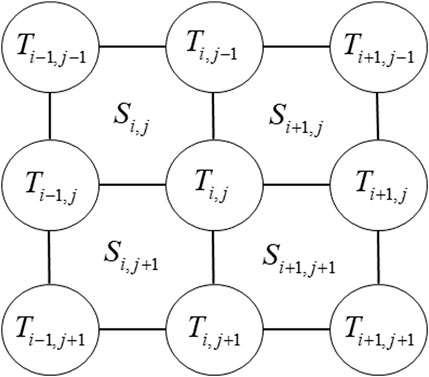
Figure 1. The grid shows the traveltimes and slowness distributions.

2.2.1 Plane wave operator

In the finite-difference scheme, the partial derivatives of Equation 4 with respect to the x- and z-directions can be represented using the following central difference formulas:

$\begin{array}{l}\frac{dT}{dx}=\frac{T_{i,j}-T_{i-1,j}+T_{i,j-1}-T_{i-1,j-1}}{2d_x}\\ \frac{dT}{dz}=\frac{T_{i,j}-T_{i,j-1}+T_{i-1,j}-T_{i-1,j-1}}{2d_z}\end{array}(5)$

$\begin{array}{l}{T}_h=T_{i-1,j}-T_{i,j-1}+T_{i-1,j-1}\\ T_{\nu }=T_{i,j-1}-T_{i-1,j}+T_{i-1,j-1}\end{array}(6)$

where T_h and T_v are variables introduced to simplify subsequent complex expressions. By incorporating Equations 5, 6 into Equation 4, followed by straightforward mathematical derivation, the first-arrival traveltimes for the plane wave can be determined as follows:

$\begin{array}{l}{T}_{i,j}=\frac{-b\pm \sqrt{b^2-4ac}}{2a},\\ a=\frac{1}{4}\left(\frac{1}{d{x}^2}+\frac{1}{d{z}^2}\right),\\ b=-\frac{1}{2}\left(\frac{T_h}{d{x}^2}+\frac{T_{\nu }}{d{z}^2}\right),\\ c=\frac{1}{4}\left(\frac{T_h^2}{d{x}^2}+\frac{T_v^2}{d{z}^2}\right)-S_{i-1,j-1}^2.\end{array}(7)$

2.2.2 Spherical wave operator

To overcome the singularity in simulating first-arrival traveltimes near the source, the solution for T(x) can be expressed as the product of a known solution and a decomposition factor. The traveltimes and slowness model are decomposed according to Equation 8:

$\begin{array}{l}T\left(x\right)=T_0\left(x\right)\tau \left(x\right)\\ S\left(x\right)=S_0\left(x\right)\alpha \left(x\right)\end{array}(8)$

If both T₀(x) and S₀(x) are known solutions, Equation 4 can be transformed to numerical evaluation of the factor $\tau \left(x\right)$, as given by Equation 9:

$T_0^2{\left|\nabla \tau \right|}^2+2T_0\tau \nabla T_0·\nabla \tau +\left({\tau }^2-{\alpha }^2\right)S_0^2=0(9)$

Equation 10 defines the boundary conditions:

$\tau \left(x\right)=\left\{\begin{array}{ll}T\left(x\right)/T_0\left(x\right),& T_0\left(x\right)\ne 0\\ \alpha \left(x\right),& T_0\left(x\right)=0\end{array}\right.(10)$

we can calculate a numerical solution for the factor τ(x), τ_h and τ_v can be obtained by replacing T with τ in Equation 6:

$\begin{array}{l}{\tau }_{i,j}=\frac{-b\pm \sqrt{b^2-4ac}}{2a},\\ a=\frac{T_0^2}{4}\left(\frac{1}{d_x^2}+\frac{1}{d_z^2}\right)+T_0\left(\frac{T_{0,x}}{d_x}+\frac{T_{0,z}}{d_z}\right)+S_0^2,\\ b=-\frac{T_0^2}{2}\left(\frac{{\tau }_h}{d_x^2}+\frac{{\tau }_{\nu }}{d_z^2}\right)-T_0\left(\frac{{\tau }_h{T}_{0,x}}{d_x}+\frac{{\tau }_{\nu }{T}_{0,z}}{d_z}\right),\\ c=\frac{T_0^2}{4}\left(\frac{{\tau }_h^2}{d_x^2}+\frac{{\tau }_v^2}{d_z^2}\right)-S_{i-1,j-1}^2.\end{array}(11)$

2.2.3 Refracted wave operator

The refracted wave operator has been developed to accurately simulate the propagation of refracted or direct waves:

$\begin{array}{l}{T}_{i,j}=\mathit{min}\left(T_{rh},T_{r\nu }\right),\\ T_{rh}=T_{i-1,j}+d_x\min \left(S_{i-1,j-1,}{S}_{i-1,j}\right),\\ T_{rv}=T_{i,j-1}+d_z\min \left(S_{i-1,j-1,}{S}_{i,j-1}\right).\end{array}(12)$

The AFDM calculates first-arrival traveltimes at each grid point using the plane wave operator from Equation 7, the spherical wave operator from Equation 11, and the refracted wave operator from Equation 12. It selects the minimum value among these three as the candidate traveltimes T_can. If T_can is smaller than the previous one, the method updates the traveltimes accordingly. This process continues until the traveltimes converge to stable values.

2.2.4 Accuracy analysis of adaptive finite-difference method

To validate the accuracy of first-arrival traveltimes computed by the AFDM, we compare AFDM with Godunov upwind difference method (Zhao, 2005) and the hybrid method (Noble et al., 2014). Since the analytical solution for traveltimes from a source in a homogeneous model can be easily derived, we construct a 60 × 60 grid homogeneous slowness model with a slowness of 0.0004 s/m. The relative errors between the numerical solutions and the analytical solution for the three methods are calculated using the Equation 13:

$Re=\frac{\left|S_{num}-S_{ana}\right|}{S_{ana}}(13)$

where Re is relative error, S_num and S_ana represent the numerical solution and the analytical solution, respectively.

Figure 2 presents the relative errors between the numerical solutions obtained by the three methods and the analytical solution. Due to source singularity, Figure 2A shows noticeable relative errors near the source for Godunov upwind difference method. In Figure 2B, the hybrid method exhibits smaller relative errors near the source owing to its windowing scheme; however, it fails to adequately handle wave propagation outside the window, resulting in significantly increased errors in those regions. In contrast, Figure 2C demonstrates that AFDM achieves substantially smaller maximum relative errors compared to the other two methods, confirming its accuracy in computing first-arrival traveltimes. Table 1 presents a comparative analysis of computational time and maximum relative errors for three different eikonal equation solvers. While AFDM requires slightly longer computation time than the other two methods - owing to its utilization of three different local operators for eikonal equation solutions - it achieves significantly smaller maximum relative errors. We contend that this marginal increase in computational overhead is well justified by the substantial improvement in first-arrival traveltimes accuracy.

Figure 2

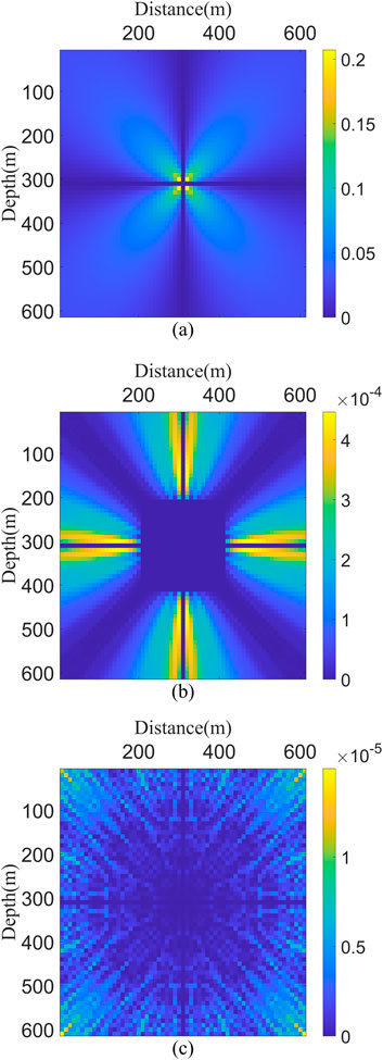
Figure 2. The relative errors between numerical solutions and analytical solutions for different eikonal equation solvers are shown for (A) Godunov upwind difference method, (B) the hybrid method, and (C) AFDM.

Table 1

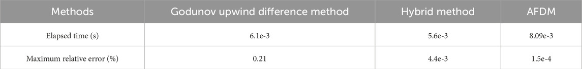
Table 1. Comparison of elapsed time and maximum relative error for three different eikonal wave equation solvers.

2.2.5 The ELNCIC based on adaptive finite-difference method

Although the first-arrival traveltimes computed using the AFDM are sufficiently accurate, the eikonal equation calculation inherently ignores the wavelet duration. Additionally, considering various sources of error in practical applications, this study adopts the following reference first-arrival traveltimes T_re is determined by Equation 14:

$T_{\text{re}}=T_{AFDM}+\frac{a}{f_m},a\in \left[1,1.25\right](14)$

where T_AFDM is first-arrival traveltimes calculated by AFDM, f_m represents dominant frequency of source wavelet, a is an error factor introduced to account for practical considerations (Wang et al., 2025).

In the LNCIC framework (Zhang et al., 2022), each grid point maintains a time window of length 2L+1 to store local wavefield. During forward and backward propagation, we preserve the source and receiver wavefield within their respective time windows, which are subsequently applied to imaging using Equation 15:

$I_{LNCIC}\left(x,z,s_j\right)={\displaystyle \sum _{i=T_{\max }-L·t_s}^{T_{\max }+L·t_s}}{p}_s\left(x,z,t_i;s_j\right)·p_r\left(x,z,t_i;s_j\right)(15)$

where I_LNCIC represents the migration image of the LNCIC, s_j denotes the jth shot, T_max refers to the excitation time, and t_i is the ith time step, t_s is the search step length proposed based on the Nyquist sampling theorem in Equation 16:

$t_s\le \frac{1}{2\left(f_{\max }-f_{\min }\right)}(16)$

where f_max and f_min represent the maximum and minimum frequency of the seismic records, respectively. To demonstrate that the excitation time used in LNCIC affects the quality of the migration image, we use the Marmousi velocity model (Figure 3) and set the source position at 2062.5 m to obtain the excitation time and single-shot migration image for analysis. Figure 4A shows the excitation time used in LNCIC, and Figure 4B presents the single-shot migration image obtained by cross-correlating the wavefield corresponding to this excitation time. It is evident in the figure that there is noticeable distortion in the migration image. We have also used arrows to highlight the locations of distortion in the migration image, which directly correspond to the disturbed positions of the excitation time. Therefore, using a more continuous and accurate first-arrival traveltimes as the excitation time will effectively improve the accuracy of the migration image. At the same time, to demonstrate the feasibility of replacing the excitation time with the first-arrival traveltimes calculated by AFDM, we set the source at the same location to obtain the first-arrival traveltimes calculated by AFDM (Figure 5A) and the single-shot migration image calculated using this time (Figure 5B). We can observe that, due to the stability and continuity of the calculated first-arrival traveltimes, there is no distortion in the migration image in Figure 5B.

Figure 3

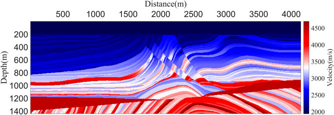
Figure 3. The velocity of Marmousi model.

Figure 4

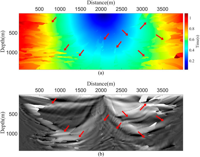
Figure 4. (A) The excitation time used in LNCIC and (B) the single-shot migration image obtained using this excitation time.

Figure 5

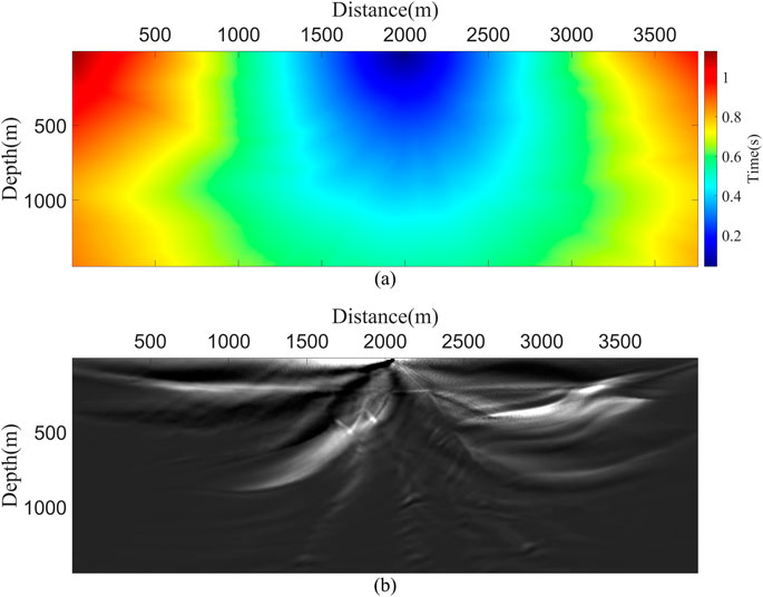
Figure 5. (A) The improved excitation time using AFDM and (B) the single-shot migration image obtained using this excitation time.

By incorporating T_re into LNCIC, we can obtain the following expression for the ELNCIC from Equation 17:

$I_{ELNCIC}\left(x,z;s_j\right)={\displaystyle \sum _{i=T_{re}-L·t_s}^{T_{re}+L·t_s}}{p}_s\left(x,z,t_i;s_j\right)·p_r\left(x,z,t_i;s_j\right)(17)$

where I_ELNCIC represents migration image of the ELNCIC. The stacked migration image is obtained by stacking the migration images from each shot.

3 Numerical examples

In the numerical examples, we compare the performance of ELNCIC with three methods: the traditional EAIC, the stable EAIC (SEAIC) (Wang et al., 2025) and SNCCIC. These comparisons are conducted using the Marmousi model, noise-contaminated data, and field data to evaluate imaging quality and robustness.

3.1 Marmousi model example

The Marmousi model has a grid size of 663 × 234 with a spatial sampling interval of 6.25 m (Figure 3). A total of 100 shots are evenly distributed along the surface, with a shot spacing of 37.5 m. A Ricker wavelet with a dominant frequency of 20 Hz is used as the source, and the recording duration is 3 s with a temporal sampling interval of 0.5 m. For the selection of the time window size, we use the period of the source wavelet, t_source, as a measure. Through our tests, we found that choosing a time window size of 3.0tsource provides high-quality imaging while maintaining relatively small computational time and disk storage requirements. The numerical examples in this paper all use this window size.

In Figure 6, we present the migration results obtained using four different imaging conditions. The images generated by EAIC (Figure 6a) exhibit significant distortion in the red rectangular region. This artifact arises from the inherent limitations of EAIC, where the maximum amplitude values in these areas may become distorted because the stored excitation amplitudes do not correspond to first-arrival waves but rather to other wave types, such as reflected or refracted waves. The resulting amplitude inconsistencies introduce severe interference during multi-shot stacking. Figure 6b demonstrates that SEAIC, which employs precise first-arrival traveltimes as excitation times, significantly reduces the distortion within the red rectangle. The migration image generated by ELNCIC (Figure 6c) not only completely resolves distortion in complex structural areas but also effectively suppresses background noise, demonstrating comparable quality to the SNCCIC result (Figure 6d). However, ELNCIC achieves this while significantly reducing storage requirements and improving computational efficiency, as it only utilizes the local source wavefield and receiver wavefield, unlike SNCCIC which requires full wavefield storage.

Figure 6

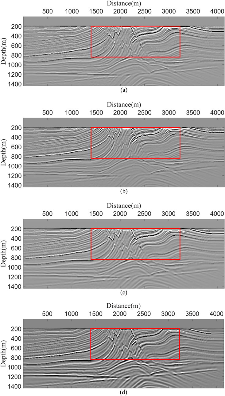
Figure 6. The stacked RTM images calculated by four different imaging condition, (a) EAIC, (b) SEAIC, (c) ELNCIC and (d) SNCCIC.

To facilitate clearer comparison and observation, we provide an enlarged view of the red rectangular region in Figure 7. Additionally, we extract two waveform traces from the migration images at x = 312.5 m and x = 1562.5 m (Figure 8). These traces provide a more intuitive comparison of the four imaging conditions. The ELNCIC results show excellent agreement with SNCCIC, while black arrows highlight the distorted regions in the EAIC and SEAIC results.

Figure 7

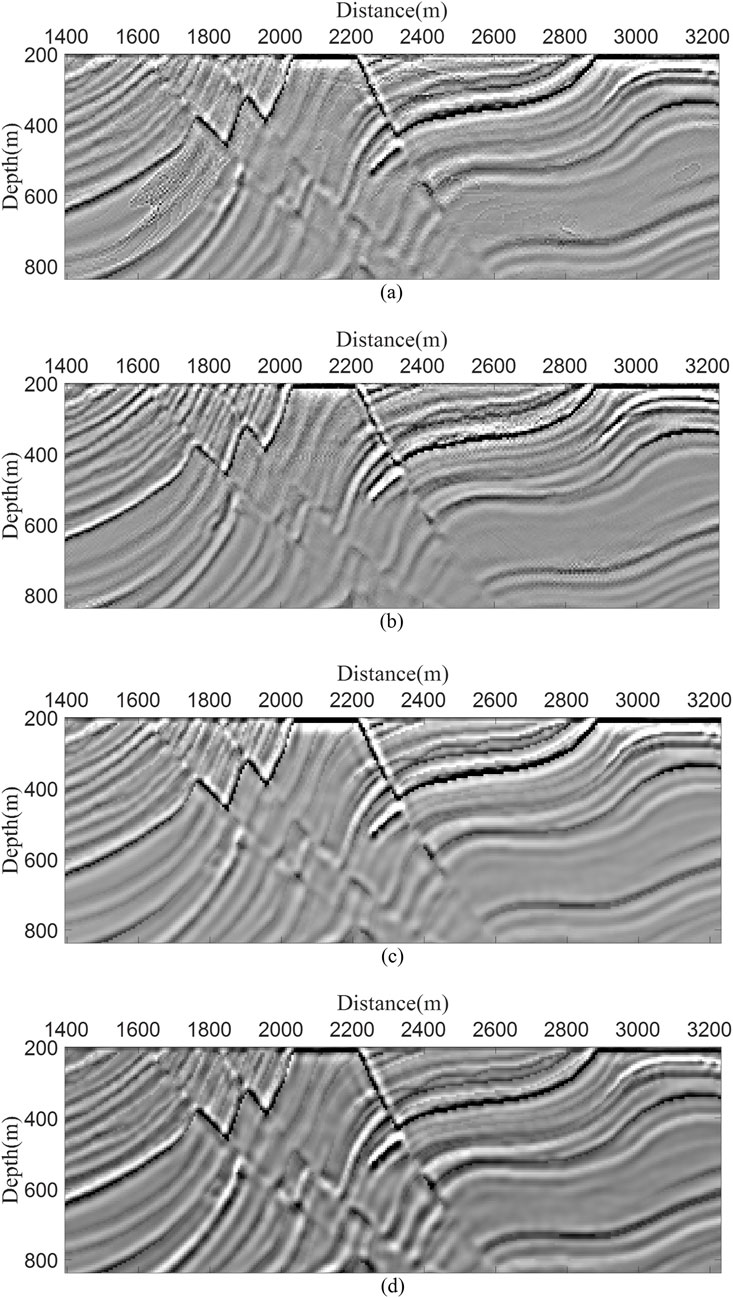
Figure 7. The enlarged views of the red rectangular regions corresponding to panels (A–D) in Figure 6.

Figure 8

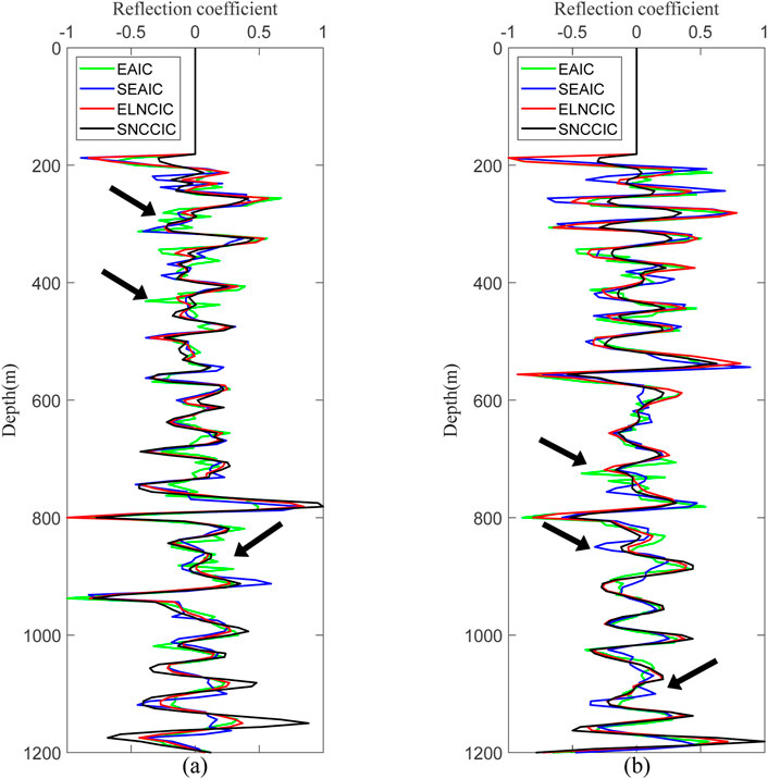
Figure 8. The waveform plot of traces located at (a) x = 312.5 m and (b) x = 1562.5 m from Figure 6. The green curve represents EAIC, the blue curve represents SEAIC, and the red curve represents ELNCIC and the black curve represents SNCCIC.

Table 2 shows the disk storage space and computation time required for the four imaging conditions. From the data in the table, it is evident that ELNCIC requires only 2.23% of the storage and 21.99% of the computation time compared to SNCCIC. Although the storage requirements and computation time for ELNCIC are slightly higher than those for EAIC and SEAIC, the resulting image quality more than justifies the increase.

Table 2

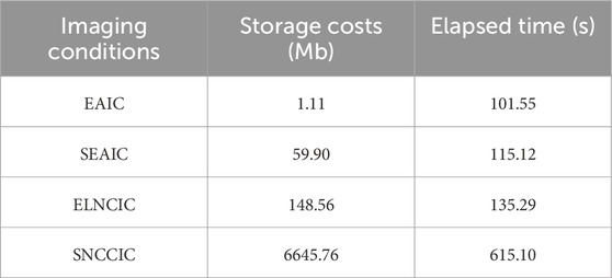
Table 2. Comparison of storage cost and elapsed time for the four imaging conditions.

3.2 Noise resistance analysis

In practice, seismic data are often severely contaminated by noise, and denoising during preprocessing may result in the loss of valuable signals. To preserve the original seismic data as much as possible, we add random Gaussian noise to the seismic records to reduce the signal-to-noise ratio (SNR). The Equation 18 gives the expression for SNR:

$\text{SNR}=10\times \lg \left(\frac{P_{signal}}{P_{noise}}\right)(18)$

where, P_signal and P_noise are represent the signal power and noise power, respectively. We set the SNR of the seismic records to 5 dB. Figure 9 compares the original seismic records and seismic records with SNR = 5 dB, revealing that some valuable signals in the seismic records are severely contaminated.

Figure 9

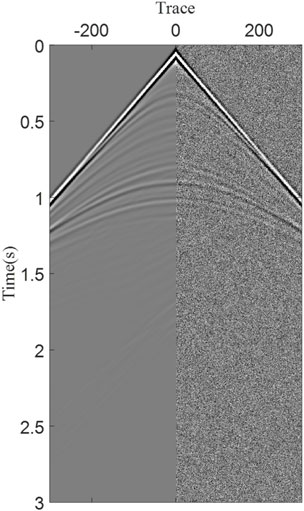
Figure 9. Single shot seismic records with Gaussian noise, the left displays the original seismic record, while the right shows the seismic record with SNR = 5 dB.

Figure 10 demonstrates the imaging performance of the four imaging conditions on noise-contaminated seismic data. EAIC exhibits poor noise resistance, causing severe contamination in the migration images, particularly in deeper layers. Although SEAIC has been improved by utilizing the highest SNR portions of the seismic data for imaging, it still fails to adequately suppress background noise. In contrast, both ELNCIC and SNCCIC significantly outperform the former two methods. ELNCIC, which not only effectively suppresses noise and enhances image quality but also substantially reduces storage requirements and improves computational efficiency compared to SNCCIC, which uses wavefields from all time steps.

Figure 10

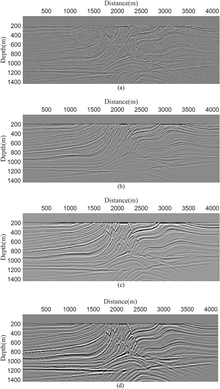
Figure 10. The stacked RTM images calculated by four different imaging condition, (a) EAIC, (b) SEAIC, (c) ELNCIC and (d) SNCCIC.

Similarly, we extracted waveform traces at x = 312.5 m and x = 1562.5 m (Figures 11a,b), using the black curve representing SNCCIC as the reference. Under noise contamination, both EAIC (green curve) and SEAIC (blue curve) exhibit significantly distorted waveforms that fail to match the reference, whereas ELNCCIC (red curve) maintains good agreement with SNCCIC, demonstrating its superior noise resistance capability.

Figure 11

Figure 11. The waveform plot of traces located at (a) x = 312.5 m and (b) x = 1562.5 m from Figure 10. The green curve represents EAIC, the blue curve represents SEAIC, and the red curve represents ELNCIC and the black curve represents SNCCIC.

3.3 Field data example

Next, we evaluate the performance of ELNCIC on field data. The velocity profile, shown in Figure 12, spans a width of 15.61 km and a depth of 5.5 km. The computational domain is discretized into a 1561 × 550 grid with a spatial sampling interval of 10 m. A total of 88 shots are unevenly distributed along the surface, with each shot recorded for 6 s at a temporal sampling interval of 0.5 m.

Figure 12

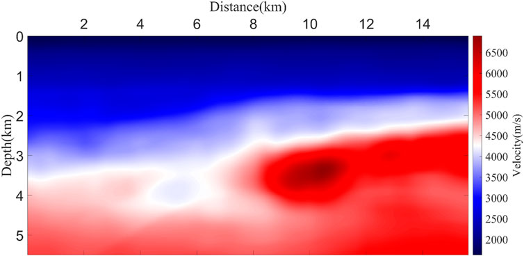
Figure 12. The velocity of field seismic data.

Figure 13 demonstrates the application of AFDM in field data. The calculated first-arrival traveltimes do not exhibit any disturbances, indicating that this method is also effective in field data. Figure 14 demonstrates the performance of the four imaging conditions on field data. The regions within the red and blue rectangles provide a clearer comparison of the differences among the four methods. Due to their reliance on wavefields only at excitation times, EAIC and SEAIC produce migration images with weaker event amplitudes, particularly below 4 km depth, where their performance is unsatisfactory. In contrast, ELNCIC, as theoretically predicted, generates images with continuous and clear stratigraphic features, achieving imaging quality comparable to SNCCIC. For a more detailed observation, enlarged views of the red rectangular regions in Figure 14 are presented in Figure 15.

Figure 13

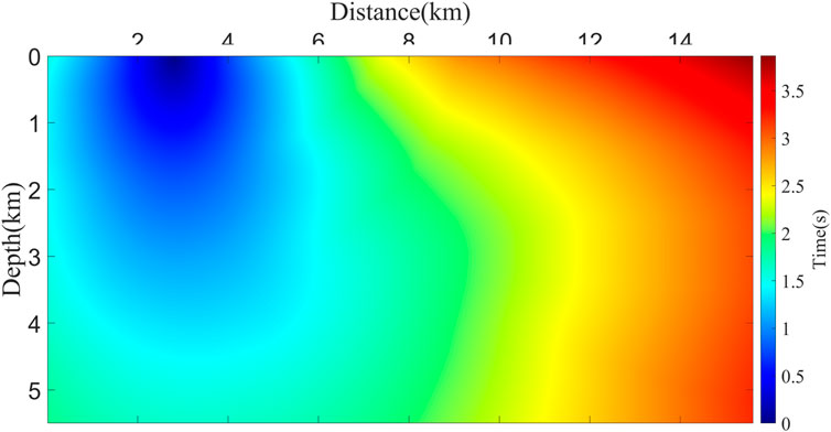
Figure 13. The first-arrival travelstimes field calculated using AFDM in the field data.

Figure 14

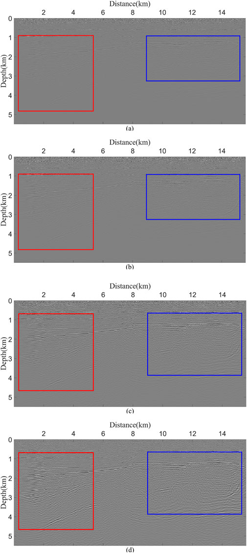
Figure 14. The stacked RTM images of field data by four different imaging condition, (a) EAIC, (b) SEAIC, (c) ELNCIC and (d) SNCCIC.

Figure 15

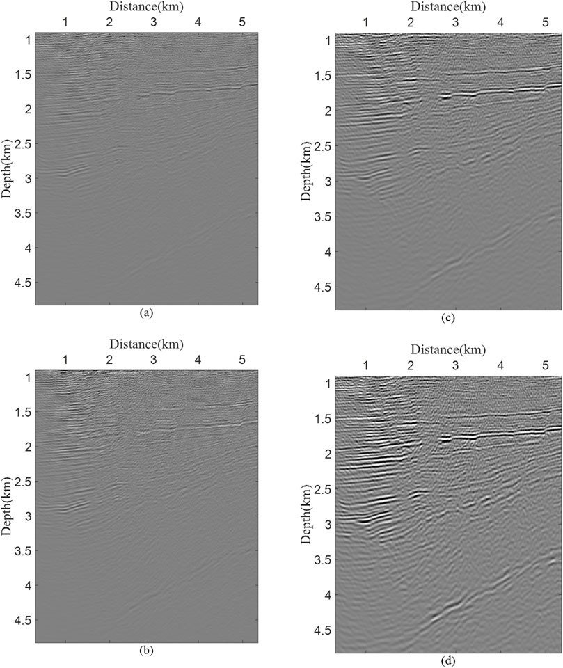
Figure 15. The enlarged views of the red rectangular regions corresponding to those in Figure 14.

4 Discussion

The ELNCIC proposed in this study, similar to EAIC and SEAIC, belongs to a specific category of cross-correlation-based imaging conditions. While EAIC and SEAIC utilize wavefield information only at excitation times for cross-correlation imaging, ELNCIC employs locally effective wavefield information. Theoretically, richer wavefield information used for cross-correlation leads to higher-quality migration images, but this comes at the cost of substantial storage requirements and high computational expenses. EAIC and SEAIC, which utilize limited wavefield information, achieve computational efficiency but offer virtually no noise resistance. Therefore, ELNCIC represents an effective compromise, delivering high-quality imaging and strong noise resistance while maintaining reasonable computational efficiency.

When addressing multi-path issues, ELNCIC can adapt by appropriately increasing the time window length, trading some computational efficiency for improved performance in complex wave propagation scenarios. While this study focuses on isotropic media, future work will extend the application to more complex media, including attenuative and anisotropic media.

5 Conclusion

The ELNCIC uses the first-arrival traveltimes, calculated by AFDM, as the excitation time. A time window is set around the excitation time, and the Nyquist sampling theorem is applied to establish the search time step. By storing the local source and receiver wavefields for imaging, it achieves low storage requirements while maintaining high-quality imaging. Through numerical experiments on the Marmousi model, noise-contaminated data, and field data, we have demonstrated ELNCIC’s superior imaging capabilities in complex geological settings and its robustness against noise.

Data availability statement

The original contributions presented in the study are included in the article/supplementary material, further inquiries can be directed to the corresponding author.

Author contributions

GL: Writing – original draft, Data curation, Methodology, Writing – review and editing. LZ: Funding acquisition, Writing – review and editing. LH: Writing – review and editing. YW: Writing – review and editing. ZQ: Writing – review and editing.

Funding

The author(s) declare that financial support was received for the research and/or publication of this article. This work is supported by the Study on identification, description and evaluation technology of ultra-deep and super-deep carbonate rock traps (P24009) and Integrated research and application of ultra-deep and super-deep drilling geological engineering (P24136).

Acknowledgments

We would like to thank the reviewers and editors for their valuable suggestions for the paper.

Conflict of interest

Authors GL, LZ, LH, YW, and ZQ were employed by Sinopec Northwest China Petroleum Bureau.

Generative AI statement

The author(s) declare that no Generative AI was used in the creation of this manuscript.

Publisher’s note

All claims expressed in this article are solely those of the authors and do not necessarily represent those of their affiliated organizations, or those of the publisher, the editors and the reviewers. Any product that may be evaluated in this article, or claim that may be made by its manufacturer, is not guaranteed or endorsed by the publisher.

References

Baysal, E., Kosloff, D. D., and Sherwood, J. W. (1983). Reverse time migration. Geophysics 48, 1514–1524. doi:10.1190/1.1441434

CrossRef Full Text | Google Scholar

Chen, G., and Wang, Z. (2018). A checkpoint-assisted interpolation algorithm of wave field reconstruction and prestack reverse time migration. Chin. J. Geophys 61, 3334–3345. doi:10.6038/cjg2018L0504

CrossRef Full Text | Google Scholar

Claerbout, J. F. (1971). Toward a unified theory of reflector mapping. Geophysics 36, 467–481. doi:10.1190/1.1440185

CrossRef Full Text | Google Scholar

Clapp, R. G. (2009). “Reverse time migration with random boundaries,” in Paper read at SEG international exposition and annual meeting.

Google Scholar

Feng, B., and Wang, H. (2012). Reverse time migration with source wavefield reconstruction strategy. J. Geophys. Eng. 9, 69–74. doi:10.1088/1742-2132/9/1/008

CrossRef Full Text | Google Scholar

Griewank, A. (1992). Achieving logarithmic growth of temporal and spatial complexity in reverse automatic differentiation. Optim. Methods Softw. 1, 35–54. doi:10.1080/10556789208805505

CrossRef Full Text | Google Scholar

Griewank, A., and Walther, A. (2000). Algorithm 799: revolve: an implementation of checkpointing for the reverse or adjoint mode of computational differentiation. ACM Trans. Math. Softw. 26, 19–45. doi:10.1145/347837.347846

CrossRef Full Text | Google Scholar

Gu, B., Liu, Y., Ma, X., Li, Z., and Liang, G. (2015). A modified excitation amplitude imaging condition for prestack reverse time migration. Explor. Geophys. 46, 359–370. doi:10.1071/eg14039

CrossRef Full Text | Google Scholar

Huang, J., Chen, L., Wang, Z., Song, C., and Han, J. (2023). Adaptive variable-grid least-squares reverse-time migration. Front. Earth Sci. 10, 1044072. doi:10.3389/feart.2022.1044072

CrossRef Full Text | Google Scholar

Kaelin, B., and Guitton, A. (2006). “Imaging condition for reverse time migration,” in Seg technical program expanded abstracts 2006 (Society of Exploration Geophysicists), 2594–2598.

Google Scholar

Komatitsch, D., and Martin, R. (2007). An unsplit convolutional perfectly matched layer improved at grazing incidence for the seismic wave equation. Geophysics 72, SM155–SM167. doi:10.1190/1.2757586

CrossRef Full Text | Google Scholar

Le Bouteiller, P., Benjemaa, M., Métivier, L., and Virieux, J. (2018). An accurate discontinuous Galerkin method for solving point-source Eikonal equation in 2-D heterogeneous anisotropic media. Geophys. J. Int. 212, 1498–1522. doi:10.1093/gji/ggx463

CrossRef Full Text | Google Scholar

Li, Q., Fu, L.-Y., Zhou, H., Wei, W., and Hou, W. (2019). Effective Q-compensated reverse time migration using new decoupled fractional Laplacian viscoacoustic wave equation. Geophysics 84, S57–S69. doi:10.1190/geo2017-0748.1

CrossRef Full Text | Google Scholar

Liu, H.-W., Liu, H., Zou, Z., and Cui, Y.-F. (2010). The problems of denoise and storage in seismic reverse time migration. Chin. J. Geophys. -Chinese Ed. 53, 2171–2180. doi:10.3969/j.issn.0001-5733.2010.09.017

CrossRef Full Text | Google Scholar

Loewenthal, D., and Mufti, I. R. (1983). Reversed time migration in spatial frequency domain. Geophysics 48, 627–635. doi:10.1190/1.1441493

CrossRef Full Text | Google Scholar

Lv, W., Du, Q., Fu, L.-Y., Li, Q., Zhang, J., and Zou, Z. (2022). A new scheme of wavefield decomposed elastic least-squares reverse time migration. Front. Earth Sci. 10. doi:10.3389/feart.2022.991093

CrossRef Full Text | Google Scholar

Nguyen, B. D., and McMechan, G. A. (2013). Excitation amplitude imaging condition for prestack reverse-time migration. Geophysics 78, S37–S46. doi:10.1190/geo2012-0079.1

CrossRef Full Text | Google Scholar

Noble, M., Gesret, A., and Belayouni, N. (2014). Accurate 3-D finite difference computation of traveltimes in strongly heterogeneous media. Geophys. J. Int. 199, 1572–1585. doi:10.1093/gji/ggu358

CrossRef Full Text | Google Scholar

Qiao, B., Pan, Z., Huang, W., and Cao, C. (2021). An adaptive finite-difference method for accurate simulation of first-arrival traveltimes in heterogeneous media. Appl. Math. Comput. 394, 125792. doi:10.1016/j.amc.2020.125792

CrossRef Full Text | Google Scholar

Sethian, J. A., and Popovici, A. M. (1999). 3-D traveltime computation using the fast marching method. Geophysics 64, 516–523. doi:10.1190/1.1444558

CrossRef Full Text | Google Scholar

Shi, Y., Ke, X., and Zhang, Y. (2015). Analyzing the boundary conditions and storage strategy for reverse time migration. Prog. Geophys. 30, 581–585. doi:10.6038/pg20150214

CrossRef Full Text | Google Scholar

Sun, W., and Fu, L.-Y. (2013). Two effective approaches to reduce data storage in reverse time migration. Comput. Geosci. 56, 69–75. doi:10.1016/j.cageo.2013.03.013

CrossRef Full Text | Google Scholar

Symes, W. W. (2007). Reverse time migration with optimal checkpointing. Geophysics 72, SM213–SM221. doi:10.1190/1.2742686

CrossRef Full Text | Google Scholar

Symes, W. W., Denel, B., Cherrett, A., Dussaud, E., Williamson, P., Singer, P., et al. (2008). “Computational strategies for reverse-time migration,” in Paper read at SEG international exposition and annual meeting.

Google Scholar

Van Trier, J., and Symes, W. W. (1991). Upwind finite-difference calculation of traveltimes. Geophysics 56, 812–821. doi:10.1190/1.1443099

CrossRef Full Text | Google Scholar

Vidale, J. E. (1990). Finite-difference calculation of traveltimes in three dimensions. Geophysics 55, 521–526. doi:10.1190/1.1442863

CrossRef Full Text | Google Scholar

Wang, J., Li, Q., Qiao, B., and Qi, J. (2025). Reverse time migration using excitation amplitude imaging condition based on accurate first-arrival traveltimes calculation. IEEE Trans. Geosci. Remote Sens. 63, 1–11. doi:10.1109/tgrs.2025.3527144

CrossRef Full Text | Google Scholar

Whitmore, N. D. (1983). Iterative depth migration by backward time propagation, SEG Technical Program expanded abstracts 1983. Society of Exploration Geophysicists, 382–385.

CrossRef Full Text | Google Scholar

Xie, C., Song, P., Li, X., Tan, J., Wang, S., and Zhao, B. (2021). Angle-weighted reverse time migration with wavefield decomposition based on the optical flow vector. Front. Earth Sci. 9. doi:10.3389/feart.2021.732123

CrossRef Full Text | Google Scholar

Zhang, M., Zhou, H., Chen, H., Jiang, S., and Jiang, C. (2022). Reverse-time migration using local nyquist cross-correlation imaging condition. IEEE Trans. Geosci. Remote Sens. 60, 1–14. doi:10.1109/tgrs.2022.3168582

CrossRef Full Text | Google Scholar

Zhao, H. (2005). A fast sweeping method for eikonal equations. Math. Comput. 74, 603–627. doi:10.1090/s0025-5718-04-01678-3

CrossRef Full Text | Google Scholar

Zhou, H.-W., Hu, H., Zou, Z., Wo, Y., and Youn, O. (2018). Reverse time migration: a prospect of seismic imaging methodology. Earth-Sci. Rev. 179, 207–227. doi:10.1016/j.earscirev.2018.02.008

CrossRef Full Text | Google Scholar

Zhu, T., and Chun, K.-Y. (1994). Understanding finite-frequency wave phenomena: phase-ray formulation and inhomogeneity scattering. Geophys. J. Int. 119, 78–90. doi:10.1111/j.1365-246x.1994.tb00914.x

CrossRef Full Text | Google Scholar