Dynamic and static integrated classification model of gas well based on XGBoost algorithm—an example from block S of Sulige tight sandstone gas field

Classification of gas wells is an important part of optimizing development strategies and increasing the recovery. The original classification standard of gas wells in the Sulige gas field has weak regularity of each parameter, large overlapping range of classification results, serious discrepancy between the dynamic and static, and low efficiency of manual classification. Aiming at this problem, this paper establishes a set of dynamic and static integrated classification model of tight sandstone gas wells in Sulige based on XGBoost algorithm. After comparison and verification, it is proved to be accurate and reliable. The model can be substituted into the static and dynamic characteristic parameters at the same time to complete the importance ranking of classification features and model training, and realize the dynamic and static integration classification of Sulige gas well. The model is applied to 553 gas wells in S block, and it is concluded that the main factors affecting the classification of gas wells are initial daily production, effective thickness of a gas layer, formation permeability, original formation pressure, and porosity. The main factors affecting the classification of class I and class II wells are initial daily production and permeability, and the main factors affecting the classification of class III wells are initial daily production and the effective thickness of the gas layer. This method improves the effectiveness of gas well classification, reduces subjectivity, and the classification results are in line with the actual situation of the field, which has guiding significance for the classification management of gas wells and the formulation of development countermeasures.

1 Introduction

Sulige tight sandstone gas reservoirs are characterized by low porosity, low permeability, and strong heterogeneity, which leads to low production and large differences in production between wells (Lu et al., 2015), so it is necessary to study the classification of tight sandstone gas wells in order better to guide the later production of tight gas wells. Many scholars have concluded that the classification methods of Sulige gas wells include: the traditional single static reservoir parameter method and test gas non-resistance flow method, single production dynamic classification method, and water production status classification (Li et al., 2011; Clarkson, 2013; Li and Huang, 2017; Sun et al., 2019; Wang et al., 2022; Zhu et al., 2024). The reservoir parameter method is based on the effective reservoir thickness to classify gas wells, which cannot dynamically reflect the actual gas wells production. The non-resistance flow is calculated by the one-point method before production, and the stable well test is rarely carried out in tight gas production, hence, this method reflects the seepage characteristics of the near-well formation fracture zone in the early stage of production, and it cannot accurately reflect the gas well production capacity. The daily gas production method does not consider the influence of production time on gas production capacity, and the unit pressure drop gas production method is affected by large fluctuations during the discontinuous production of gas wells, so it has great limitations. In the actual production, the single dynamic and static classification method has low manual classification efficiency, and the classification results of dynamic and static parameters are very different. In addition, the current mathematical processing methods of classification include the fuzzy mathematics method, grey correlation method, cumulative deviation coefficient, and so on (Jin, 2019; Zhu et al., 2019; Liu et al., 2020; Feng et al., 2021; Liang et al., 2021), but the setting of weight coefficients in these methods has a certain degree of human factors and is not sufficiently objective.

In terms of oil and gas well classification techniques, in the early days, traditional statistical and empirical formulae methods were mainly used in combination with static geologic parameters, such as porosity, permeability and gas saturation to carry out classification studies (Archie, 1942; Garb, 1985; Arps, 1945) divided oil and gas wells into different production types by analyzing the production decline curve. Ershaghi and Omorigie (1978) evaluated the production dynamics of oil and gas wells by examining the relationship between water content and cumulative production. Sharma et al. (2010) performed linear regression analysis within the identified cluster analysis and compared it with Arps empirical correlation; the study showed that geological and engineering parameters are correlated, and both are important for oil and gas well classification and recovery prediction. However, traditional statistical techniques make it difficult to handle complex nonlinear relationships and do not effectively combine static data with dynamic production data. With the development of computer technology, (Li et al., 2010) used SVM to classify the production dynamics of oil and gas wells, and the results showed that SVM has high classification accuracy when dealing with nonlinear data. Al-Anazi and Gates (2010b), Al-Anazi and Gates (2010a) applied SVM to the production capacity prediction of tight gas reservoirs and found that it outperformed the traditional regression model. Ahmadi and Chen (2019) used random forests to classify the production data of oil and gas wells and successfully identified high-yield wells and low-yield wells. Although machine learning methods have demonstrated strong performance in oil and gas well classification, model training requires a large amount of high-quality data with limited ability to handle missing and noisy data.

In recent years, with the development of big data and deep learning techniques, the classification methods of oil and gas wells have become more accurate and sophisticated (Mohammadpoor and Torabi, 2020; Ibrahim et al., 2022; Zhao et al., 2024) proposed a gas well type prediction method based on two-dimensional convolutional neural network (2D-CNN) to solve the problem of low prediction accuracy of tight sandstone gas well type evaluation method. Sun et al. (2020), Hu et al. (2023) used a convolutional neural network (CNN) to classify seismic data and successfully identified the distribution characteristics of oil and gas reservoirs. Song et al. (2020) applied the Long Short-Term Memory Network (LSTM) to classify the production dynamics of oil and gas wells, which was able to capture the long-term dependency in time series data effectively. XGBoost, as an efficient integrated learning algorithm (Chen and Guestrin, 2016), excels in handling high-dimensional data, nonlinear relationships, and missing data by integrating multiple weak classifiers. It can efficiently capture the nonlinear relationship and importance between features, and reduce bias and variance. However, 2D-CNN is difficult to accurately fit the classification boundary without sufficient data or feature engineering support. Wang et al. (2021) combined XGBoost with LSTM to construct a hybrid model for classifying gas wells in tight sandstone, and the results showed that it outperformed a single model. Liu et al. (2021) combined Random Forest with Deep Learning to construct a multi-task learning model for shale gas capacity prediction and classification. Zhang et al. (2023a), Zhang et al. (2023b), Lin et al. (2025) predicted the capacity of different classes of gas wells by constructing a segmented production model.

Scholars have conducted extensive and in-depth research on oil and gas well classification, promoting the transformation of classification methods from traditional statistical analysis to modern machine learning methods. However, the conventional static geological model and dynamic production data analysis are often independent of each other, which makes it difficult to reflect the real situation of gas wells fully. Moreover, Sulige gas wells have weak regularity to the parameters in the original classification standard (mainly based on the effective thickness of gas wells, test gas non-resistance flow rate, initial daily gas production, porosity, and permeability), which leads to a large range of overlapping classification results. The situation of dynamic and static inconsistency is more serious. Therefore, it is urgent to construct a classification model for tight sandstone gas wells that can combine dynamic and static data to improve the field development efficiency and optimize the production strategy.

In this paper, to address the problems of inconsistency between dynamic and static and low time efficiency of manual classification, a set of dynamic and static integrated classification models for tight sandstone gas wells is established based on the XGBoost algorithm by combining static geological parameters (as thickness of the gas layer, permeability) and dynamic production data (as production rate, pressure). The model is accurate and reliable, can effectively overcome the defects of a single classification method, can improve the timeliness of the classification work, and can provide powerful support for the countermeasures of gas field development.

2 Model establishment

This chapter first introduces the principle and process of the XGBoost algorithm. Then, it selects the input feature parameters substituted into the model training through correlation analysis and data standardization of the collected feature data, and the gas well classification features are ranked of importance. Then, the standardized data are divided into training sets and test sets to classify the gas wells, respectively, and the indexes of the three classification results are evaluated. Finally, a reliable classification model of Sulige tight sandstone gas wells is obtained.

2.1 Principle and process of XGBoost algorithm

2.1.1 Algorithm principle

The XGBoost algorithm (Chen and Guestrin, 2016) can effectively use the extracted features to integrate several weak classifiers into a strong classifier through multiple rounds of iteration and residual fitting, which has good generalization performance and high computational efficiency. The XGBoost algorithm is a gradient-boosting decision tree (GBDT) algorithm, which starts from the second tree during training and learns the residual sum of all previous tree conclusions. This residual sum is the amount of cumulative error obtained through the predicted values of all previous trees, which can make the expected results closer to the correction of the true value. Compared with other commonly used machine learning methods [such as support vector machine (Li et al., 2010) and random forest (Ahmadi and Chen, 2019)], XGBoost has better classification performance and is not easily affected by the quality of training data.

The XGBoost algorithm improves the overall classification performance by combining multiple weak classifiers through weighted summation, the expression is (Equation 1) (the formula is derived in Supplementary Appendix):

$\widehat{y_i}={\displaystyle \sum _{k=1}^K}{f}_k\left(x_i\right),\left(f_k\in F\right)(1)$

2.1.2 Modeling process

Using the XGBoost algorithm to carry out machine learning modeling for the classification of tight gas wells, which mainly contains four steps of data preprocessing, feature selection, model construction and analysis, and evaluation of the training model, the specific process is shown in Figure 1. Firstly, the field data are collected, the data correlation analysis is carried out, and the data set is standardized. The characteristic parameters substituted into the model training are screened. Then, the data is divided into a training set (80%) and a test set (20%) to classify gas wells respectively, and the importance of gas well classification features is ranked. Finally, the index of the three classification results is evaluated. A reliable XGBoost classification model is obtained.

Figure 1

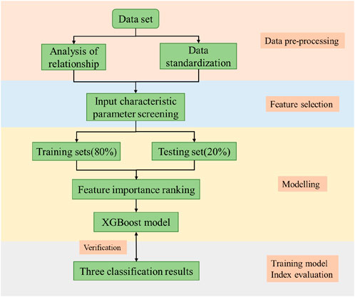
Figure 1. XGBoost algorithm flow diagram.

According to the commonly used gas well classification indexes in the Sulige gas field, eight dynamic and static characteristics of gas layer thickness $h$, porosity $\varphi$, permeability $k$, gas saturation $S_g$, original formation pressure $P_i$, non-resistance flow $Q_{AO}$, initial daily production $Q_i$ , and casing pressure before production $P_c$ are taken as the input characteristics of the classification model to form a training data set. The classification results of gas wells are taken as the output characteristics for training.

2.2 Data processing and analysis

This study uses the data of 450 gas wells in Sulige tight sandstone gas reservoir. These gas wells are located in the northeastern end of Sulige gas field, with an area of 615 km². The geographical location is located in Wushenqi, Inner Mongolia Autonomous Region. The surface environment is mostly desert and grassland. The static geological characteristic parameters, dynamic production parameters and field classification results were collected. When conducting sample learning, the field classification results are used as evaluation samples for performance evaluation and verification of the XGBoost algorithm.

Descriptive statistical analysis of the original data collected on site to clarify the characteristics of the data set. The characteristic parameters are input, and the mean, standard deviation, maximum value, minimum value, are taken as the output to obtain the descriptive statistical table (Table 1) and the box line diagram (Figure 2).

Table 1

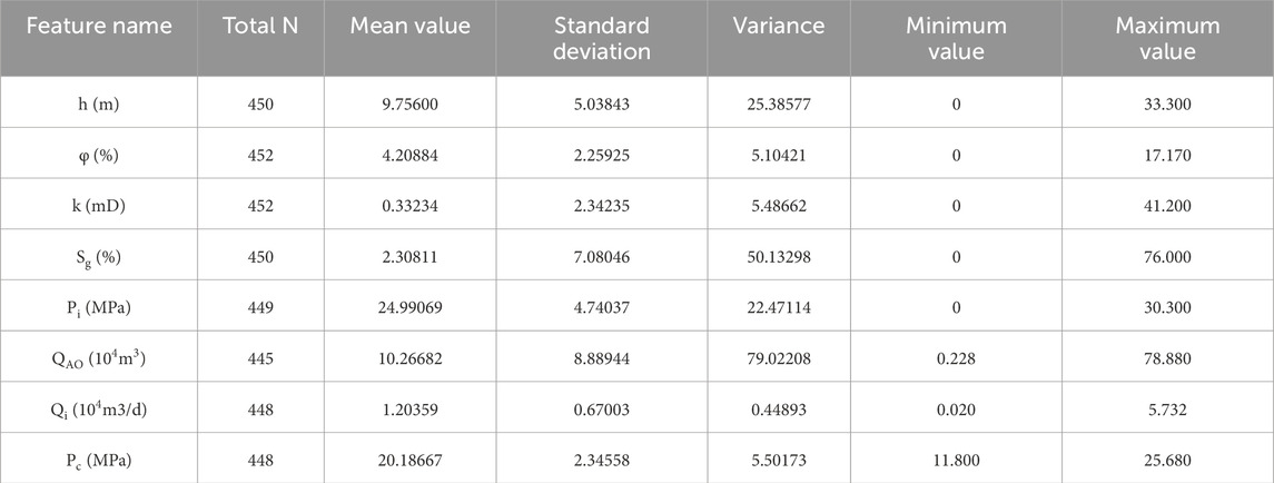
Table 1. Statistical table of characteristic parameter description.

Figure 2

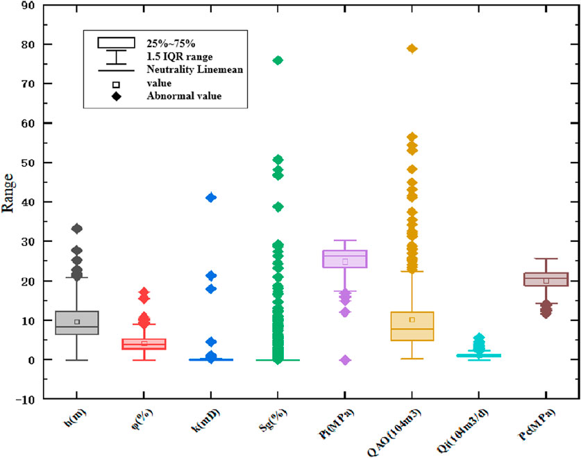
Figure 2. Box line diagram.

It can be seen from Table 1 that except for the number of samples of h and S_g is 450, the remaining variables are between 445 and 452, and there may be a small number of missing values. The mean value of Pi is 24.99 MPa, which is close to the maximum value of 30.3 MPa, indicating that most of the data are distributed in the high pressures range. The mean value of k is 0.332 mD, but the maximum value is 41.2 mD, indicating the existence of extremely high permeability samples, which may be fractured reservoirs or data errors. However, the model may regard this abnormal value as a high-permeability or high-yield gas well, which makes the model unable to distinguish the geological model of fracture-dominated wells from matrix-dominated wells. The S_g variance is 50.13 (standard deviation 7.08), and the dispersion is the highest, indicating that the saturation distribution is extremely uneven. The P_c variance is 5.50 (standard deviation 2.35), the data is relatively concentrated and the stability is good. The minimum values of h, φ, k, S_g, and Pi are all 0, and check whether they are valid measurements. The data points distributed outside the 1.5 IQR data range are outliers. From the box plot of Figure 2, it can be seen that there are outliers in each variable, of which S_g and Q_AO are the most. Next, it is recommended to process the original data through data standardization methods.

2.2.1 Data correlation analysis

Before importing data, before importing the data, the Pearson correlation coefficient is used to analyze the correlation of the data, and the relationship between the two variables can be viewed through the matrix scatter plot (Figure 3). On the diagonal, the histogram of each corresponding variable shows the distribution of each input feature. It can be seen from Figure 3 that there is no obvious linear relationship between most variables, which increases the difficulty of analysis. It can be seen from the histogram that each feature does not show a normal distribution. Before the subsequent model training, the data should be standardized and mapped into normal distribution to avoid the impact of data distribution on model training.

Figure 3

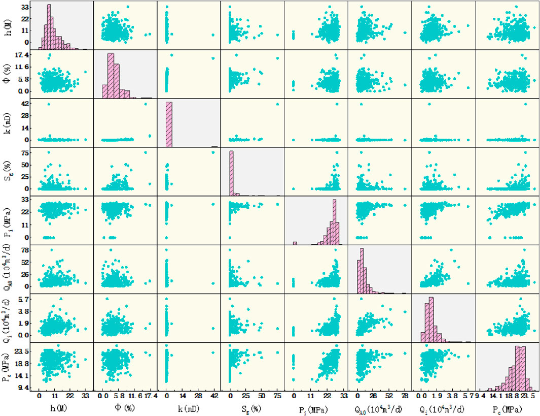
Figure 3. Scatter plot of the matrix of characteristic parameters.

The data samples of the Sulige gas field are drawn into a heat map, and the results are shown in Figure 4. The heat map is a statistical chart that displays data by coloring the color blocks. It consists of two classification domains and a numerical domain. Among them, the classification field determines the horizontal and vertical axes, and divides the chart into regular rectangular blocks; the range determines the color of the rectangular block. The depth of the color can represent the value or number of data points, with reddish colors indicating smaller values and bluish colors indicating larger values. As can be seen in Figure 4, there is a positive correlation between non-resistance flow and initial flow and a weak negative correlation between formation thickness and porosity. Since providing the same information for the model may result in a confusing model, it is necessary to consider whether there are features with extremely high correlation coefficients, that is, collinear features. Figure 4 shows that each feature provides different information, so all features are substituted into the model for training.

Figure 4

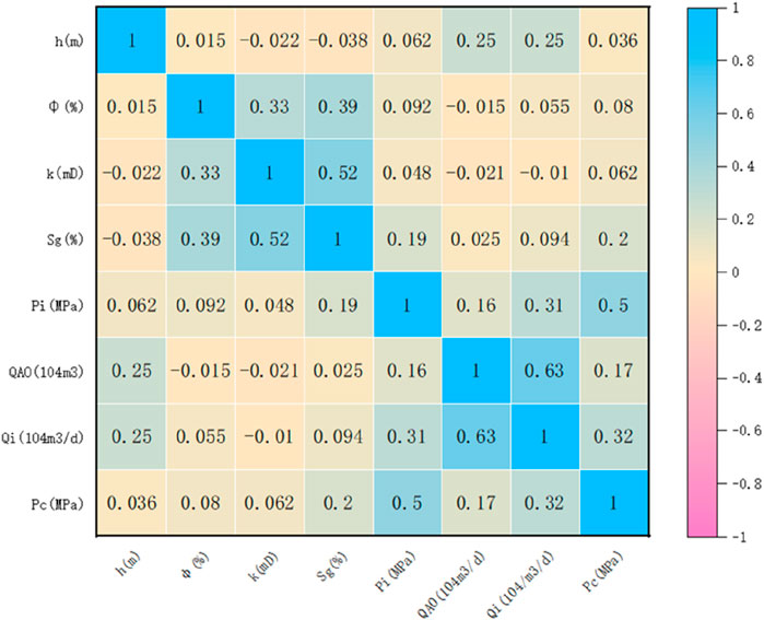
Figure 4. Heat map of characteristic parameters.

2.2.2 Data standardization

In the descriptive statistical analysis of the original feature data, it is found that there are outliers, and the data needs to be standardized, that is, the attributes of the samples need to be scaled to some specified range. In addition to the tree-based algorithm, the other algorithms of the XGBoost algorithm require zero mean and unit variance of the samples, and need to eliminate the influence of different attributes and different orders of magnitude of the samples. After standardization, the optimal value calculation process range is reduced, the steps are gentle, and it is easier to converge to the optimal solution correctly.

Data standardization methods include MinMaxScaler method (Ambarwari et al., 2020), RobustScaler method (Ahsan et al., 2021), and StandardScaler method (Nabi, 2016). After investigation, it is found that the MinMaxScaler method needs to strictly limit the range, which is greatly affected by outliers and destroys the original distribution. The RobustScaler method is suitable for data with a large number of outliers, but the standardized data variance is not 1, which may affect the convergence speed of the linear part of XGBoost. StandardScaler (based on Z-score normalization) is a widely used normalization method, especially suitable for XGBoost or other machine learning algorithms that are sensitive to data distribution. The data can be converted to a standard normal distribution with a mean of 0 and a standard deviation of 1. The expression is Equations 2, 3:

$S_t\left(X\right)=\frac{X-\mu }{\delta }(2)$

$X=\left[\begin{array}{l}{x}_1\\ x_2\\ ⋮\\ x_n\end{array}\right](3)$

The advantages and rationality of selecting StandardScaler are as follows: First, it can be compatible with the numerical stability requirements of XGBoost.Through the unified dimension, all features are in the same order of magnitude, so as to avoid some features dominating model training due to excessive values. Second, the interpretability of outliers can be retained. After standardization, outliers will be compressed to a certain range (such as Z-score >3), but their statistical significance will be retained. If the original anomaly value of k is 41.2 mD, it may become 15.3 mD (Z-score) after standardization, but it can still be identified. Third, it meets the implicit requirements of XGBoost for zero mean and unit variance. Fourth, it can improve the convergence efficiency of gradient descent.

For each sample attribute, it is operated by a column, subtracting the average value and then dividing it by the standard deviation in order to standardize the data. For missing values, the median and mode are filled, and the outliers are deleted or replaced with the mean. The above operation makes the new dataset have a variance of 1 and an average value of 0. After standardizing the original data, the data obeys the normal distribution, as shown in Figure 5.

Figure 5

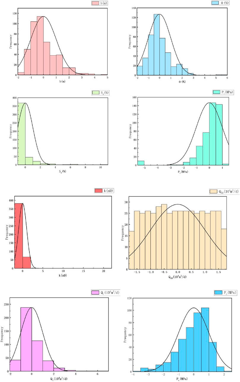
Figure 5. Normal distribution plot of characteristic parameters.

2.3 Static-dynamic integrated gas well classification model

2.3.1 Gas well classification model

The standardized data set is divided into 80% for training and 20% for testing, resulting in a training data set of 360 samples and a testing data set of 90 samples in this study. The model parameters of the training output as shown in Table 2. The training set contains 77 Class I wells, 198 Class II wells, and 85 Class III wells; the test set includes 14 Class I wells, 52 Class II wells, and 24 Class III wells.

Table 2

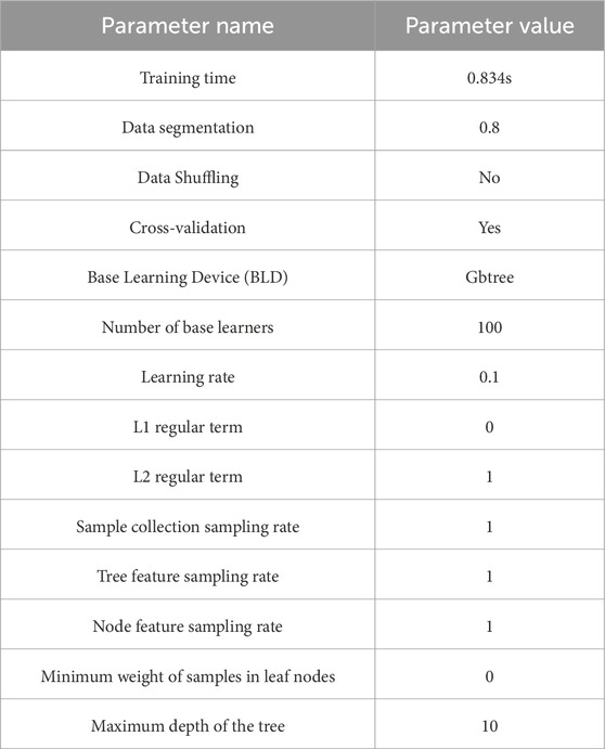
Table 2. Model parameters.

Using the XGBoost classifier trained on 360 datasets, we compare predicted and actual values to generate the confusion matrix heat map (Figure 6). The Confusion matrix is one of the most commonly used indicators for evaluating the performance of a multiclassification model. The confusion matrix provides a clearer understanding of the performance of the classifier on different categories. Each of its columns represents the predicted category, and the total number of each column indicates the number of data predicted to be in that category; each row represents the true attributed category of the data, and the total numbers of data in each row indicates the number of data instances in that category.

Figure 6

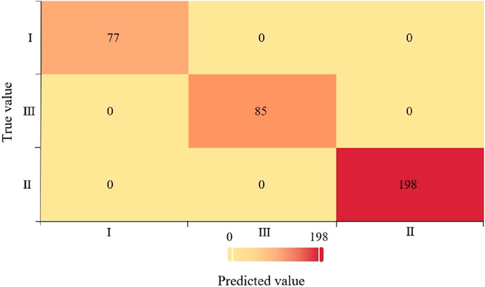
Figure 6. Confusion matrix heat map of training data.

The Ⅰ, Ⅱ, and Ⅲ on the axes of the confusion matrix heat map in Figure 6 represent Class I wells, Class II wells, and Class III wells, respectively; the numbers on the diagonal of the matrix indicate the number of correctly categorized wells, and the remaining numbers indicate the number of misclassified wells.

The 90 test sample data are tested by the formed XGBoost training model, resulting in the confusion matrix heat map shown in Figure 7. From the figure, it can be seen that there are five Class II wells in the real data that are shown to be Class I wells in the prediction, and one Class I well in the real data that is shown to be a Class II well in the prediction.

Figure 7

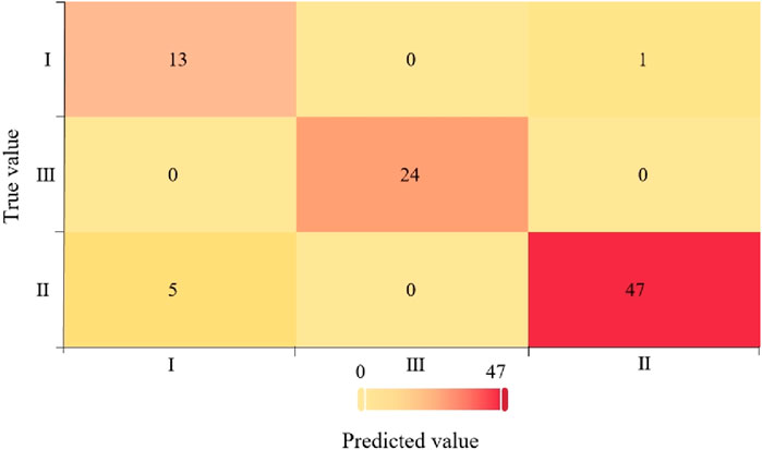
Figure 7. Confusion matrix heat map of test data.

In addition to confusion matrix heat maps, commonly used classification evaluation indicators include accuracy, recall, precision, and F₁ value.

The accuracy expression is Equation 4:

$A_{cc}=\frac{TP+TN}{TP+TN+FP+FN}(4)$

The recall rate expression is Equation 5:

${{\mathrm{R}}_e}_e=\frac{TP}{TP+FN}(5)$

The accuracy rate is expressed as Equation 6:

${P_r}_e=\frac{TP}{TP+FP}(6)$

The $F_1$ value is the harmonic mean of precision and recall, which takes the range of [0,1]. Usually, the higher its value, the better the performance of the algorithm and its expression is Equation 7:

$F_1=2\frac{P_{re}{R}_{ec}}{P_{re}+R_{ec}}(7)$

A classification report is generated from the above classifier prediction results and true values, which contain indicators such as precision, recall, $F_1$ value, and AUC support. Table 3 shows the prediction evaluation indicators for the cross-validation set, the training set, and the test set to measure the prediction effect of XGBoost through quantitative indicators. In XGBoost classification evaluation indicators, the greater the accuracy rate, recall rate, and precision rate, the better in which the precision rate and recall rate affect each other. Suppose the precision rate is high and the recall rate is low, or the recall rate is low and the precision rate is high. It is necessary to take both into account, which the $F_1$ index can be evaluated; the closer the AUC value is to 1, the better the classification effect is.

Table 3

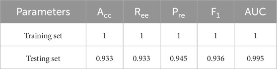
Table 3. Evaluation results of model indicators.

When constructing the XGBoost classification model, the selection of hyperparameters has a significant impact on the performance of the model. The optimal solution is found by adjusting the parameters through grid search and cross-validation to ensure a reliable and stable model. The range of tuning parameters is shown in Table 4.

Table 4

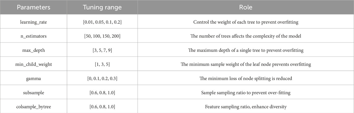
Table 4. Value range of tuning parameters.

In the tuning process, the initial coarse tuning, fixed learning_rate = 0.1, adjusted n_estimators and max_depth, and observed the performance of the model in the validation set. Then fine tuning, based on the coarse tuning results, adjust the parameters such as min_child_weight and gamma to optimize the F1 value. Re-regularization optimization, adjust subsample and colsample_bytree to prevent overfitting. Finally, the learning_rate is reduced and n_estimators are added to further improve the generalization ability. The comparative analysis of the tuning results is shown in Table 5.

Table 5

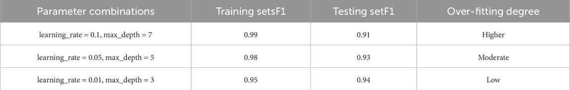
Table 5. Comparative analysis of tuning results.

According to the comparison of the optimization results, the final selection parameter combination is: learning_rate:0.05, n_estimators:150, max_depth:5, min_child_weight:3, gamma:0.1, subsample:0.8, colsample_bytree:0.8. Reducing learning_rate and increasing n_estimators make the model more stable, and the test set F1 is increased to 0.936. Restricting max_depth and min_child_weight effectively prevents overfitting, that is, the training set F1 = 1, the test set F1 = 0.933. AUC = 0.995 indicates that the model classification boundary is clear and suitable for gas well classification tasks. This tuning process ensures the high accuracy and reliability of the XGBoost model in gas well classification.

Through analyzing the confusion matrix heat map, 84 of the 90 samples in the test set are correctly classified, and six are incorrectly classified. The final classification results of the test set are obtained as shown in Table 6. It can be seen that class III wells can be completely categorized, and the $F_1$ values of class I and II wells are all above 0.8, which is a better categorization effect.

Table 6

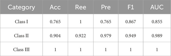
Table 6. Evaluation results of indicators for each class of well.

The XGBoost classification model is utilized to classify the characteristics of the sample wells in the Sulige gas field, such as initial daily production, the effective thickness of the gas layer, formation permeability, original formation pressure, and porosity. The boundary values of the characteristics of various classes of gas wells are shown in Table 7. So far, the dynamic and static integrated classification model of Sulige tight sandstone gas wells has been constructed.

Table 7

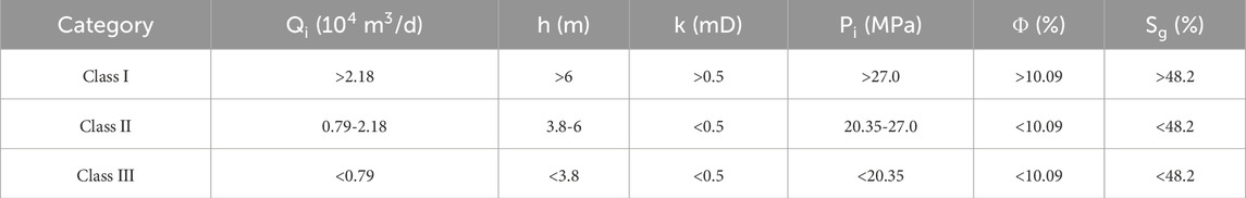
Table 7. Characteristic boundary values for various classes of gas wells.

2.3.2 Feature importance ranking

Before training the model, the XGBoost algorithm’s ‘feature importance’ attribute was used to rank the classification features of the selected eight categories of gas wells, and the results are shown in Table 8: the initial daily production has the highest importance on the gas wells classification, followed by effective thickness of the gas layer. Q_i is affected by reservoir energy, permeability and fluid mobility, and can directly capture the recoverability of the reservoir. The Q_i of high-yield wells and low-yield wells is significantly different, and the model is easy to classify by this feature. According to Darcy’s law, the production of gas wells is proportional to h, and large thickness means higher production and longer stable production period. The importance of casing pressure before production is the lowest, and the impact on gas wells is the smallest. For example, the P_c of constant pressure production wells is limited to the classification contribution.

Table 8

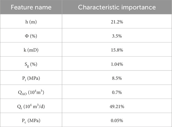
Table 8. Sorting table of gas well classification characteristics.

3 Model validation

The data of 30 wells in the S block of the Sulige gas field, which are well classified by experts’ experience, are taken. Eight dynamic and static characteristics of gas layer thickness, porosity, permeability, gas saturation, original formation pressure, non-resistance flow rate, initial daily production, and casing pressure before production are integrated. The characterization data and classification results are shown in Table 9, among which there are 9 Class I wells, 13 Class II wells, and 8 Class III wells. The data from these 30 gas wells are now substituted into the model established in this paper and the 2D-CNN gas well classification prediction model (Zhao et al., 2024) to classify the gas wells respectively. The classification results of each model and empirical classification results are shown in Table 10 and Figure 8.

Table 9

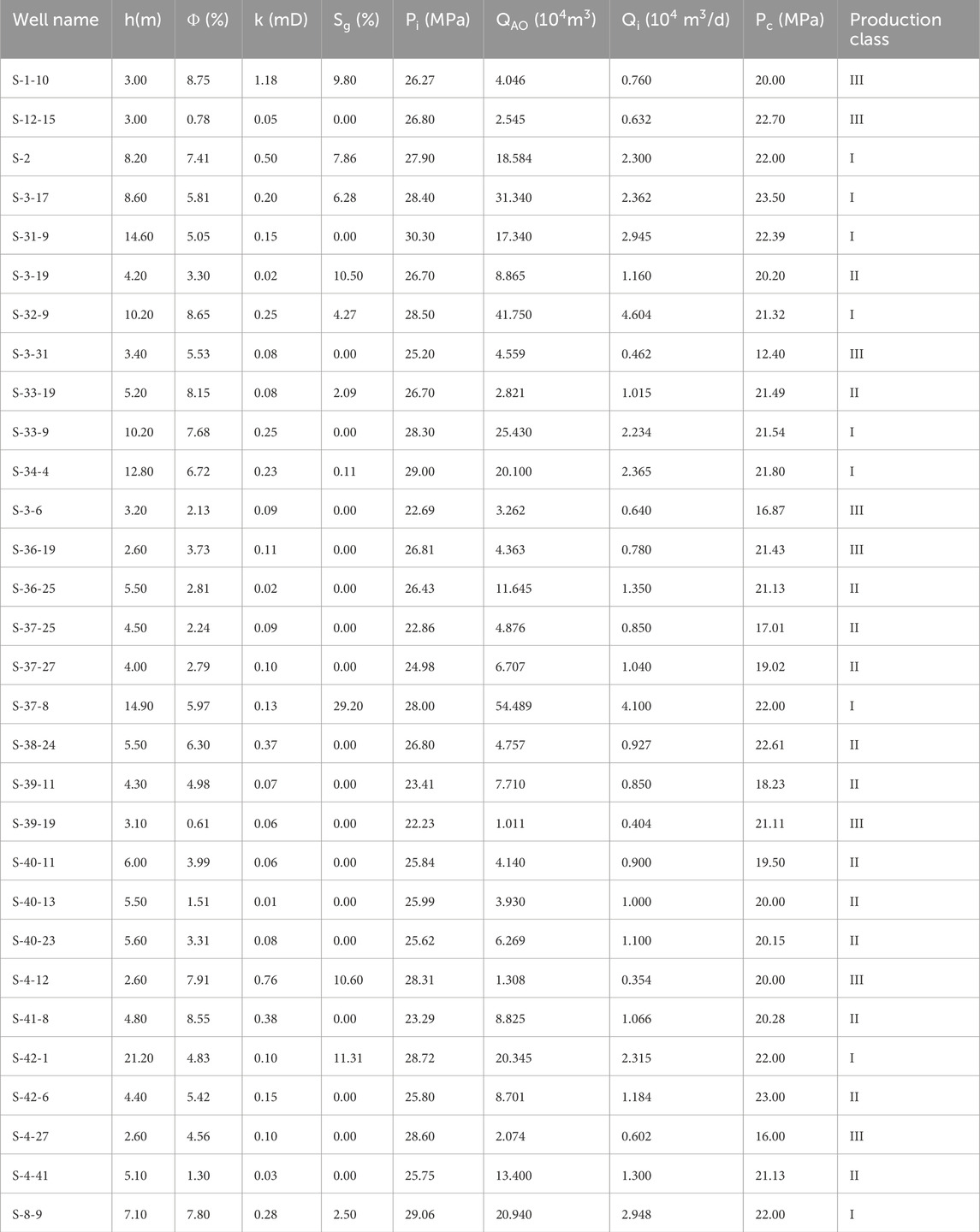
Table 9. Some gas well data of the S block in the Sulige gas field.

Table 10

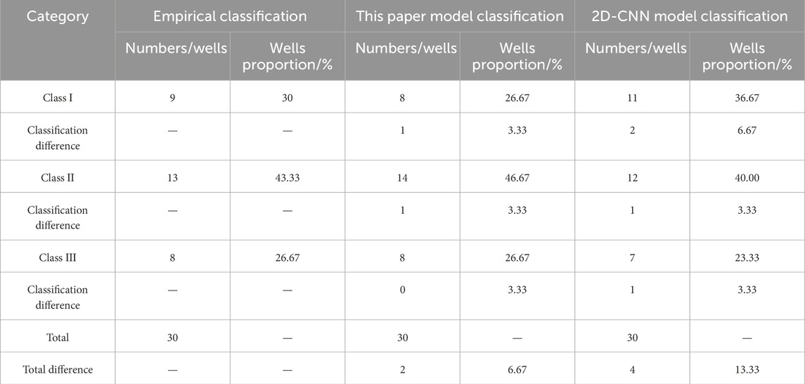
Table 10. Comparison table of model classification results and empirical classification results.

Figure 8

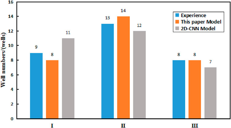
Figure 8. Comparison of classification results.

The 30 wells classified better by the expert experience are classified by the model of this paper, which results in 8, 14, and 8 wells of class Ⅰ, Ⅱ, and Ⅲ, respectively, accounting for 26.67%, 46.67%, and 26.67%, respectively. The difference between the model classification results and the Ⅰ, Ⅱ, Ⅲ class wells classified by experts’ experience is 1, 1, 0 wells respectively, and the accuracy of the gas well classification model established in this paper reaches 93.33%. Through the classification of 2D-CNN model, it is concluded that there are 11, 12 and 7 wells in class I, II and III respectively, accounting for 36.67%, 40% and 23.33% respectively. The classification results of the model are different from those of class I, II and III wells classified by expert experience by 2, 1 and 1 respectively. The accuracy of 2D-CNN gas well classification model reaches 86.67%. In contrast, the accuracy of the model in this paper is higher.

The classification of I, II and III types of gas wells depend on complex nonlinear relationships. XGBoost algorithm can efficiently capture the nonlinear relationship and importance between features, and reduce deviation and variance. However, 2D-CNN is difficult to accurately fit the classification boundary without sufficient data or feature engineering support, such as misjudging 2 Class I wells and 1 Class II and Class III wells. Compared with the high-dimensional calculation of 2D-CNN, XGBoost is more efficient in the training and reasoning stages and is more suitable for field applications.

4 Discussion and analysis of results

4.1 Discussion of model classification method

Based on the gas well dynamic and static integration classification model constructed above, 553 gas wells in block S of the Sulige gas field are now classified according to the model classification rules, and the results are shown in Table 11. The classification indexes of different class of gas wells are obtained, and are shown in Table 12.

Table 11

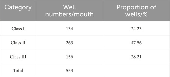
Table 11. S block gas well classification results.

Table 12

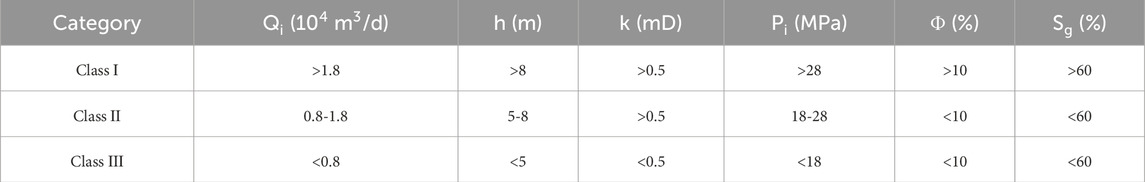
Table 12. S block gas well classification results.

According to the order of feature importance, the main factors are initial daily production, the effective thickness of a gas layer, formation permeability, original formation pressure, and porosity. Class I wells have high original gas content, good seepage conditions, and large effective gas layer thickness. The reservoir physical properties of class II wells are slightly worse, and the original gas content is lower; the characteristic parameters affecting the classification of class I and class II wells are initial daily production and permeability. The reservoir physical property of class III well is poor, and the effective reservoir thickness is the smallest. Compared with class I and class II wells, the main factors affecting class III wells are initial daily production and the effective thickness of a gas layer.

In the practice of S block, the model has a high recognition accuracy (F1-score >0.85) for Class I and Class II wells, mainly due to the ability to capture nonlinear relationships; the feature importance ranking (initial daily Q_i > h > k) is consistent with the geological understanding, which verifies the physical rationality. However, the recall rate of Class III wells is low (about 0.72), because of its dynamic data noise, such as intermittent production, resulting in production fluctuations. The model classification method successfully integrates geological static and production dynamic parameters, and solves the problem of dynamic and static inconsistency in traditional classification. The classification boundary values in Table 10 can be directly used for on-site production allocation decision. However, there are also some limitations. The model is not embedded in the seepage equation constraint, which may lead to anti-physical interpretation. In the later stage, it can be considered in the direction of ‘XGBoost + physical constraint’ hybrid modeling.

4.2 Discussion on the characteristics of various gas wells

The production pressure change curve (Figure 9) is drawn by drawing the production date of the gas well in the S block. From the production pressure change curve, it can be seen that the average production in the first 3 years is 0.66 × 10⁴ m³/d, and the average casing pressure at the end of the 3 years is 8.42 MPa. In the early stage, the pressure drop rate was 0.0286 MPa/d, and the production was gradually stable in the later stage, and the pressure drop rate was 0.0020 MPa/d. At present, the average cumulative gas production of a single well is 1,229 × 10⁴ m³. There is no obvious stable production period for the wells, and it decreases rapidly at the initial stage and shows a decreasing trend year by year with the extension of the production time. The production characteristics of various classified gas wells and typical well characteristics are discussed and analyzed, and corresponding development countermeasures are given as follows:

Figure 9

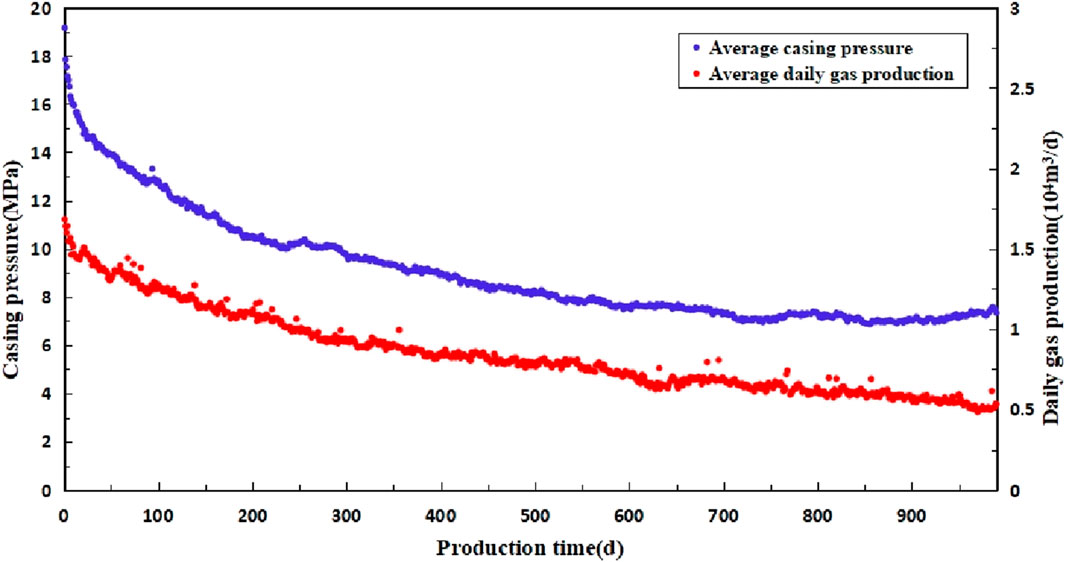
Figure 9. Production pressure change curve of vertical well in S block.

4.2.1 Class I well production characteristics and development countermeasures

There are 134 Class I wells in Block S, accounting for 24.23% of the total number of wells. The production pressure change curve (Figure 10) is drawn by the production date of class I. It can be seen that the average production of the first 3 years is 1.11 × 10⁴ m³/d, and the average casing pressure at the end of the 3 years is 7.35 MPa. The pressure drop rate is 0.0398 MPa/d in the early stage, and the pressure drop rate is 0.0025 MPa/d in the later stage. At present, the average cumulative gas production of a single well is 2,346 × 10⁴ m³. This kind of gas well can be produced continuously and has a certain stable production capacity. Still, it is necessary to control the pressure drop rate to delay the stable production period.

Figure 10

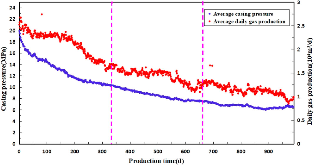
Figure 10. Production pressure change curve of class I well in S block.

Typical Class Ⅰ well (S12-6-9 well): this well box eight single pressing single testing, the non-resistance flow rate of 20.94 × 10⁴ m³/d, initial daily production of 2.95 × 10⁴ m³/d, the initial casing pressure of 20.99 Mpa, the current daily output of 0.31 × 10⁴ m³/d, the current casing pressure of 3.34 Mpa, the cumulative gas production of 7,903 × 10⁴ m³. This well was put into production on 9/27/2007; the continuous production time is a long 7-year pressure drop rate of 0.0035 MPa/d; later, into the naturally decreasing intermittent production, the production effect is good (Figure 11).

Figure 11

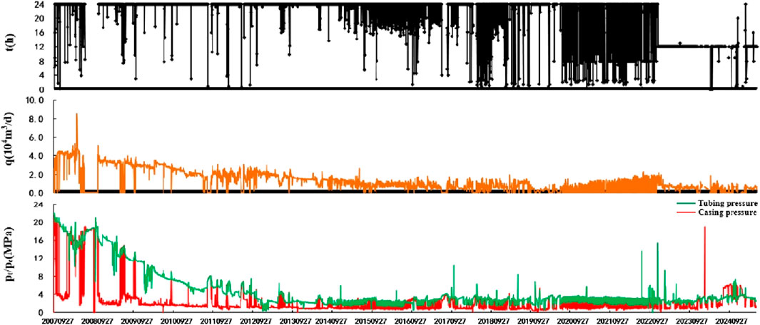
Figure 11. Production curve of Well S12-6-9.

Class Ⅰ wells have a large thickness of gas layer, with a non-resistance flow rate of 20.94 × 10⁴ m³/d, which is much higher than the average value, reflecting the high permeability characteristics of the reservoir, and high reservoir physical properties. Although Class I wells have good reservoir conditions, with the extension of production time, fracture heterogeneity may lead to insufficient local energy supply, and permeability decreases with production (such as the permeability of S12-6-9 well decreases by 35% after 7 years). If the initial production is high, it is easy to cause pressure drop rate differentiation (0.0025∼0.04 MPa/d), which affects the prediction of stable production period. If multi-layer commingled production technology is used in production, it will lead to low permeability layer inhibiting the productivity of high permeability layer.

Development countermeasures should be optimized in stages to address geological, dynamic and engineering uncertainties. Early high production stage: optimized production allocation, adjusted to 0.8∼1.5 × 10⁴ m³/d; adjust the pressure data in real time, slow down the pressure drop rate and prolong the stable production period; for wells with large differences in fracture development, gradient pressurization is adopted, and the initial production is limited by 50%, and the production is gradually increased after 3 months. Medium-term stable production stage: using layered mining technology to reduce interlayer interference; for wells with a pressure drop rate greater than 0.04 MPa/d, nitrogen is injected to delay energy depletion. Late decline stage: based on the Arps decline model and economic factors, the intermittent production system is formulated.

4.2.2 Class Ⅱ well production characteristics and development countermeasures

There are 263 Class II wells, accounting for 47.56% of the total number of wells; the average production in the first 3 years is 0.61 × 10⁴ m³/d, and the set pressure at the end of 3 years is 8.74 MPa. The pressure drop rate in the early stage is faster 0.0283 MPa/d, and the production in the later stage is gradually smooth, and the pressure drop rate is 0.0020 MPa/d. At present, the average cumulative gas production in a single well is at 1,042 × 10⁴ m³. This kind of well can basically be produced continuously, and the stable production capacity is general (Figure 12).

Figure 12

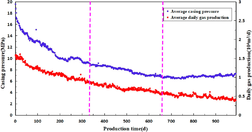
Figure 12. Production pressure change curve of class II well in S block.

Typical Class Ⅱ well (well S10-5-3): this well box eight upper box eight lower hill two three-layer split-pressing and combined testing, non-resistance flow rate of 7.6716 × 10⁴ m³/d, initial daily production of 1.17 × 10⁴ m³/d, the initial casing pressure of 19.47 Mpa, the current daily output of 0.15 × 10⁴ m³/d, the current casing pressure of 5.40 Mpa, the cumulative production of 2,090 × 10⁴ m³. This well was put into production on 10/8/2014, with an initial continuous production pressure drop rate of 0.030 MPa/d and intermittent output after 2 years, with zigzag fluctuation of the casing pressure and better production effect (Figure 13).

Figure 13

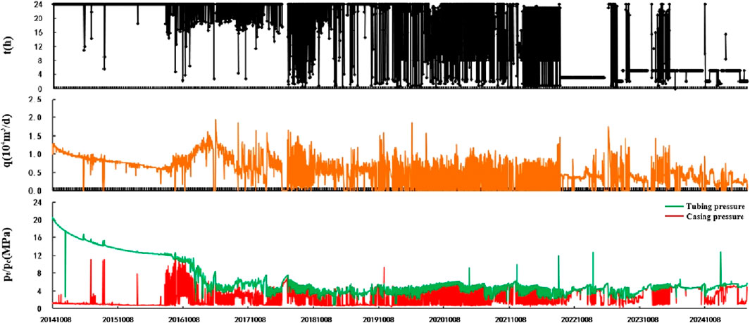
Figure 13. Production curve of Well S10-5-3.

Class II wells have small reservoir thickness, poorer physical properties than Class I wells, and lower production. There are geological uncertainties in the development, and local abrupt changes in reservoir thickness can lead to insufficient energy supply in some wells, as well as uneven fracture development, affecting the effect of fracturing and reforming. The fluctuation of pressure drop rate is large (0.005∼0.015 MPa/d), and it is difficult to stabilize production with conventional production allocation. Liquid-carrying capacity is poor, and the risk of wellbore fluid accumulation increases with the decrease of production. There is a risk of gas flaring in gas injection and development projects.

In view of the geological, dynamic and engineering uncertainties of such gas wells, in the early production stage: adjust the nozzle size to modulate the pressure drop rate of ≤0.01 MPa/d; for reservoirs <5 m in thickness, the initial production rate is reduced by 20%. In the middle stable production stage: by means of foam drainage, for wells with oil casing differential pressure > 2MPa, inject foaming agent (concentration 0.5%∼1%) to improve fluid-carrying efficiency; restore the pressure by injecting nitrogen; and for the combined wells, use layered modulation to reduce the interlayer interference. Late decreasing stage: screening wells with cumulative gas production >1,500 × 10⁴ m³ and permeability decline >30% (such as S10-5-3), repeat fracturing using low-injury fracturing fluids to explore the remaining potential.

4.2.3 Class Ⅲ well production characteristics and development countermeasures

There are 156 Class III wells, accounting for 28.21% of the total number of wells; the average production in the first 3 years is 0.30 × 10⁴ m³/d, and the casing pressure at the end of the 3 years is 8.90 MPa. The rate of pressure drop in the early stage is faster at 0.0202 MPa/d, and then the production in the later stage gradually stabilizes, with the rate of pressure drop being 0.0014 MPa/d. The casing pressure is increased in the last stage due to the influence of liquid discharge. At present, the average cumulative gas production of a single well is 584 × 10⁴ m³, and this kind of well has low production, fast pressure dropping, and a short period of stabilized production (Figure 14).

Figure 14

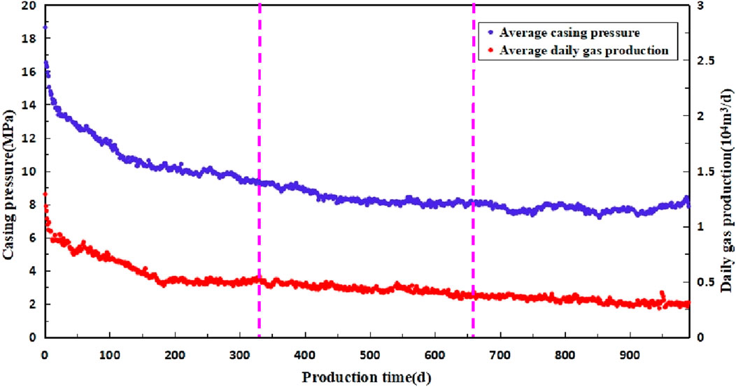
Figure 14. Production pressure change curve of class III well in S block.

Typical Class III well (well S6-40-12): this well box eight uphill one combined testing, non-resistance flow rate 1.4 × 10⁴ m³/d, initial daily production 0.59 × 10⁴ m³/d, initial casing pressure 13.54 Mpa, current daily production 0.02 × 10⁴ m³/d, current casing pressure 6.69 Mpa, cumulative gas production 380 × 10⁴ m³. The well was put into production on 3/5/2012, and the casing pressure has been climbing for a period of continuous output. Now, it is intermittent production with a general production effect (Figure 15).

Figure 15

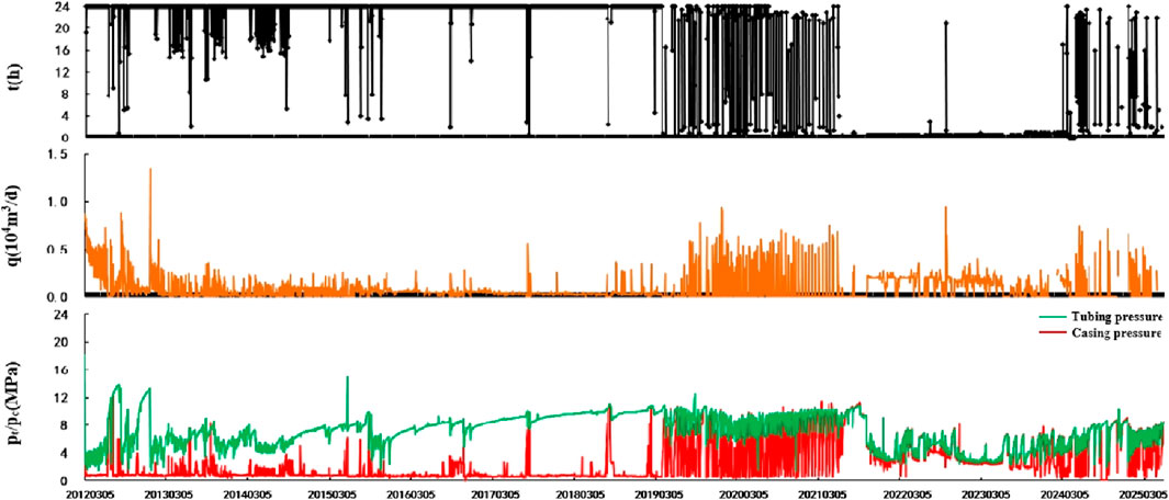
Figure 15. Production curve of Well S6-40-12.

Class III wells have poor reservoir physical properties with minimal effective thickness and permeability. The permeability of such wells is generally <0.1 mD, effective thickness <3m, natural fractures are not developed, and non-homogeneity is strong, resulting in a sudden drop in production capacity of the local well area. The rate of pressure drop is fast (0.0202 MPa/d), resulting in a short period of stabilized production. Typical well S6-40-12, the casing pressure of the well is climbing, indicating that the wellbore is seriously fluid-accumulated, which affects the normal production of the gas well. Conventional fracturing modification effect is poor, and gas injection development is easy to gas scram.

In response to geological, dynamic and engineering uncertainties, in the early production stage, the initial production rate was lowered to 0.4 × 10⁴ m³/d (60% of the initial rate of 0.65 × 10⁴ m³/d) to optimize the development plan and delay the steady production period; adaptive throttling technology was adopted, and 3 mm nozzles were used for production when the casing pressure was >8 MPa, and 2 mm nozzles and wellhead boosting were switched when the casing pressure was ≤8 MPa to maintain the production differential pressure <3 MPa. Medium-term production stabilization stage: supplement formation energy through CO₂ foam pressure drive and nano-microsphere modulation drive; activate pulse fracturing for layers <2 m in thickness, and carry out intelligent production control. Later stage of extended production: switch to intermittent production for wells with daily production <0.1 × 10⁴ m³/d and casing pressure <4 MPa; consider nitrogen throughput technology in combination with economic factors.

5 Summary and conclusion

In this paper, an integrated dynamic-static classification model for tight sandstone gas wells is established based on the XGBoost algorithm by combining dynamic and static data, which accomplishes fast and high-precision classification of gas wells. The model not only solves the problems of classification results inconsistency between dynamic and static but also improves the effectiveness of gas well classification and reduces human subjectivity. The following conclusions are mainly drawn:

(1) By analyzing the data of 450 gas wells, it was found that there was no obvious linear relationship between static and dynamic parameters of gas wells, which could be substituted into the model training and based on the feature importance screening of the XGBoost algorithm, three important indexes affecting the classification of gas wells were obtained: the initial daily production, the effective thickness of the gas layer and the permeability.

(2) Through data preprocessing, feature selection, model training and prediction, and index evaluation, a dynamic and static integrated classification model for tight sandstone gas wells was established. The results were compared and verified with those of wells that were classified better by experts’ experience, and it was concluded that the classification model was accurate and reliable.

(3) The main factors influencing the classification of Class I and II wells are initial daily production and permeability. In contrast, the main factors influencing the classification of Class III wells are initial daily production and the effective thickness of the gas layer.

(4) For Class I and II wells, the development strategy is mainly constant production, slowing down the rate of pressure drop and delaying the period of stabilized production through rational production allocation; for Class III wells, the development strategy is mainly intermittent production and drainage gas recovery to restore production capacity.

Data availability statement

The original contributions presented in the study are included in the article/Supplementary Material, further inquiries can be directed to the corresponding author.

Author contributions

SZ: Conceptualization, Data curation, Formal Analysis, Investigation, Methodology, Software, Writing – original draft, Writing – review and editing. XY: Conceptualization, Methodology, Writing – review and editing. XG: Data curation, Formal Analysis, Writing – review and editing. DL: Formal Analysis, Software, Writing – review and editing. SH: Conceptualization, Methodology, Writing – review and editing.

Funding

The author(s) declare that financial support was received for the research and/or publication of this article. The authors are very grateful to CNPC Bohai Drilling Company Limited and China University of Petroleum (Beijing) for supporting this paper. The authors declare that this study received funding from CNPC Bohai Drilling Company Limited. The funder was not involved in the study design, collection, analysis, interpretation of data, the writing of this article, or the decision to submit it for publication.

Acknowledgments

The authors would like to thank Yu Xiangdong and Huang Shijun for their interpretation of the significance of the results of this study.

Conflict of interest

Authors SZ, XY, XG, and DL were employed by CNPC Bohai Drilling Engineering Company.

The remaining author declares that the research was conducted in the absence of any commercial or financial relationships that could be construed as a potential conflict of interest.

Generative AI statement

The author(s) declare that no Generative AI was used in the creation of this manuscript.

Publisher’s note

All claims expressed in this article are solely those of the authors and do not necessarily represent those of their affiliated organizations, or those of the publisher, the editors and the reviewers. Any product that may be evaluated in this article, or claim that may be made by its manufacturer, is not guaranteed or endorsed by the publisher.

Supplementary material

The Supplementary Material for this article can be found online at: https://www.frontiersin.org/articles/10.3389/feart.2025.1605793/full#supplementary-material

References

Ahmadi, M. A., and Chen, Z. (2019). Comparison of machine learning methods for estimating permeability and porosity of oil reservoirs via petro-physical logs. Petroleum 5, 271–284. doi:10.1016/j.petlm.2018.06.002

CrossRef Full Text | Google Scholar

Ahsan, M. M., Mahmud, M. A. P., Saha, P. K., Gupta, K. D., and Siddique, Z. (2021). Effect of data scaling methods on machine learning algorithms and model performance. Technologies 9, 52. doi:10.3390/technologies9030052

CrossRef Full Text | Google Scholar

Al-Anazi, A., and Gates, I. D. (2010a). A support vector machine algorithm to classify lithofacies and model permeability in heterogeneous reservoirs. Eng. Geol. 114, 267–277. doi:10.1016/j.enggeo.2010.05.005

CrossRef Full Text | Google Scholar

Al-Anazi, A., and Gates, I. D. (2010b). On the capability of support vector machines to classify lithology from well logs. Nat. Resour. Res. 19, 125–139. doi:10.1007/s11053-010-9118-9

CrossRef Full Text | Google Scholar

Ambarwari, A., Adrian, Q. J., and Herdiyeni, Y. (2020). Analysis of the effect of data scaling on the performance of the machine learning algorithm for plant identification. J. RESTI Rekayasa Sist. Dan. Teknol. Inf. 4, 117–122. doi:10.29207/resti.v4i1.1517

CrossRef Full Text | Google Scholar

Archie, G. E. (1942). The electrical resistivity log as an aid in determining some reservoir characteristics. Trans. AIME 146, 54–62. doi:10.2118/942054-g

CrossRef Full Text | Google Scholar

Arps, J. J. (1945). Analysis of decline curves. Trans. AIME 160, 228–247. doi:10.2118/945228-g

CrossRef Full Text | Google Scholar

Chen, T., and Guestrin, C. (2016). “XGBoost: a scalable tree boosting system,” in Proceedings of the 22nd ACM SIGKDD international conference on knowledge discovery and data mining (New York, NY, USA: Association for Computing Machinery), 785–794.

Google Scholar

Clarkson, C. R. (2013). Production data analysis of unconventional gas wells: review of theory and best practices. Int. J. Coal Geol. 109–110, 101–146. doi:10.1016/j.coal.2013.01.002

CrossRef Full Text | Google Scholar

Ershaghi, I., and Omorigie, O. (1978). A method for extrapolation of cut vs recovery curves. J. Petroleum Technol. 30, 203–204. doi:10.2118/6977-pa

CrossRef Full Text | Google Scholar

Feng, S., Xie, R., Zhou, W., Yin, S., Deng, M., Chen, J., et al. (2021). A new method for logging identification of fluid properties in tight sandstone gas reservoirs based on gray correlation weight analysis — a case study of the Middle Jurassic Shaximiao Formation on the eastern slope of the Western Sichuan Depression, China. Interpretation 9, T1167–T1181. doi:10.1190/int-2020-0247.1

CrossRef Full Text | Google Scholar

Garb, F. A. (1985). Oil and gas reserves classification, estimation, and evaluation. J. Petroleum Technol. 37, 373–390. doi:10.2118/13946-pa

CrossRef Full Text | Google Scholar

Hu, Z., Bai, F., Wang, H., Sun, C., Li, P., Li, H., et al. (2023). Deep learning approaches in tight gas field pay zone classification. (OnePetro).

Google Scholar

Ibrahim, N. M., Alharbi, A. A., Alzahrani, T. A., Abdulkarim, A. M., Alessa, I. A., Hameed, A. M., et al. (2022). Well performance classification and prediction: deep learning and machine learning long term regression experiments on oil, gas, and water production. Sensors 22, 5326. doi:10.3390/s22145326

PubMed Abstract | CrossRef Full Text | Google Scholar

Jin, H. (2019). Application of fuzzy mathematical evaluation method in classification and evaluation of condensate gas reservoir. Nat. Environ. Pollut. Technol. 18.

Google Scholar

Li, B., Artemiou, A., and Li, L. (2011). Principal support vector machines for linear and nonlinear sufficient dimension reduction. Ann. Stat. 39. doi:10.1214/11-aos932

CrossRef Full Text | Google Scholar

Li, T., and Huang, X. (2017). Classification of horizontal wells based on dynamic data and its application in ultra-low permeability gas reservoirs. Chem. Technol. Fuels Oils 53, 123–134. doi:10.1007/s10553-017-0787-5

CrossRef Full Text | Google Scholar

Li, X., Cervantes, J., and Yu, W. (2010). “A novel SVM classification method for large data sets,” in 2010 IEEE international conference on granular computing, 297–302.

Google Scholar

Liang, X., Xie, Q., He, M., Liu, Q., and Morozov, V. (2021). Reservoir characteristics and its comprehensive evaluation of gray relational analysis on the western Sulige gas field, ordos basin, China. Geofluids 2021, 1–12. doi:10.1155/2021/6641609

CrossRef Full Text | Google Scholar

Lin, H., Liu, W., Zhang, D., Chen, B., and Zhang, X. (2025). Study on the degradation mechanism of mechanical properties of red sandstone under static and dynamic loading after different high temperatures. Sci. Rep. 15, 11611. doi:10.1038/s41598-025-93969-4

PubMed Abstract | CrossRef Full Text | Google Scholar

Liu, S., Chen, G., Lou, Y., Zhu, L., and Ge, D. (2020). A novel productivity evaluation approach based on the morphological analysis and fuzzy mathematics: insights from the tight sandstone gas reservoir in the Ordos Basin, China. J. Petrol Explor Prod. Technol. 10, 1263–1275. doi:10.1007/s13202-019-00822-2

CrossRef Full Text | Google Scholar

Liu, Y.-Y., Ma, X.-H., Zhang, X.-W., Guo, W., Kang, L.-X., Yu, R.-Z., et al. (2021). A deep-learning-based prediction method of the estimated ultimate recovery (EUR) of shale gas wells. Petroleum Sci. 18, 1450–1464. doi:10.1016/j.petsci.2021.08.007

CrossRef Full Text | Google Scholar

Lu, T., Liu, Y., Wu, L., and Wang, X. (2015). Challenges to and countermeasures for the production stabilization of tight sandstone gas reservoirs of the Sulige Gasfield, Ordos Basin. Nat. Gas. Ind. B 2, 323–333. doi:10.1016/j.ngib.2015.09.005

CrossRef Full Text | Google Scholar

Mohammadpoor, M., and Torabi, F. (2020). Big Data analytics in oil and gas industry: an emerging trend. Petroleum 6, 321–328. doi:10.1016/j.petlm.2018.11.001

CrossRef Full Text | Google Scholar

Nabi, Z. (2016). “Machine learning at scale,” in Pro spark streaming: the zen of real-time analytics using Apache spark. Editor Z. Nabi (Berkeley, CA: Apress), 177–198.

CrossRef Full Text | Google Scholar

Sharma, A., Srinivasan, S., and Lake, L. W. (2010). Classification of oil and gas reservoirs based on recovery factor: a data-mining approach.

Google Scholar

Song, X., Liu, Y., Xue, L., Wang, J., Zhang, J., Wang, J., et al. (2020). Time-series well performance prediction based on Long Short-Term Memory (LSTM) neural network model. J. Petroleum Sci. Eng. 186, 106682. doi:10.1016/j.petrol.2019.106682

CrossRef Full Text | Google Scholar

Sun, J., Slang, S., Elboth, T., Larsen Greiner, T., McDonald, S., and Gelius, L.-J. (2020). A convolutional neural network approach to deblending seismic data. GEOPHYSICS 85, WA13–WA26. doi:10.1190/geo2019-0173.1

CrossRef Full Text | Google Scholar

Sun, S. Z., Hou, X., Ji, L., Yang, L., and Zhu, X. (2019). Tight sand gas geophysical classification. 3498, 3502. doi:10.1190/segam2019-3216167.1

CrossRef Full Text | Google Scholar

Wang, B., Li, T., Xu, N., Zhou, H., Xiong, Z., and Long, W. (2021). “A novel reservoir modeling method based on improved hierarchical XGBoost,” in 2021 IEEE 5th advanced information technology, electronic and automation control conference (IAEAC), 1918–1923.

Google Scholar

Wang, Z., Nie, X., Zhang, C., Wang, M., Zhao, J., and Jin, L. (2022). Lithology classification and porosity estimation of tight gas reservoirs with well logs based on an equivalent multi-component model. Front. Earth Sci. 10. doi:10.3389/feart.2022.850023

CrossRef Full Text | Google Scholar

Zhang, S., Guo, K., Yang, H., and Gao, X. (2023a). The productivity segmented calculation model of perforated horizontal wells considering whether to penetrate the contaminated zone. Front. Earth Sci. 11, 1270662. doi:10.3389/feart.2023.1270662

CrossRef Full Text | Google Scholar

Zhang, S., Guo, K., and Zhang, Z. (2023b). Segmented superimposed model of near-bore reservoir pollution skin factor for low porosity and permeability sandstone horizontal gas wells. Front. Earth Sci. 11, 1335629. doi:10.3389/feart.2023.1335629

CrossRef Full Text | Google Scholar

Zhao, C., Jia, Y., Qu, Y., Zheng, W., Hou, S., and Wang, B. (2024). Forecasting gas well classification based on a two-dimensional convolutional neural network deep learning model. Processes 12, 878. doi:10.3390/pr12050878

CrossRef Full Text | Google Scholar

Zhu, P., Zhu, Z., Zhang, Y., Sun, L., Dong, Y., Li, Z., et al. (2019). Quantitative evaluation of low-permeability gas reservoirs based on an improved fuzzy-gray method. Arab. J. Geosci. 12, 80. doi:10.1007/s12517-019-4231-5

CrossRef Full Text | Google Scholar

Zhu, Z., Han, G., Liang, X., Chang, S., Yang, B., and Yang, D. (2024). Rapid classification and diagnosis of gas wells driven by production data. Processes 12, 1254. doi:10.3390/pr12061254

CrossRef Full Text | Google Scholar

Glossary

$\mathit{i}$ The index of the samples, i takes all the samples in the training phase, is used to compute the loss function and gradient, and in the prediction phase, is used to predict the sample labels

$\widehat{{\mathit{y}}_{\mathit{i}}}$ Prediction results for sample xi

$\mathit{K}$ Number of weak classifiers

${\mathit{f}}_{\mathit{k}}$ kth weak classifier

$\mathit{F}$ The set of all possible weak classifiers

${\widehat{\mathit{y}}}_{\mathit{i}}^{\left(\mathit{t}\right)}$ Sample prediction results for the tth iteration

$\mathit{t}$ tth iteration

${\displaystyle \mathbf{\text{∑}}_{\mathit{i}\mathbf{\text{=}}\mathbf{1}}^{\mathit{n}}}\mathit{l}\left({\mathit{y}}_{\mathit{i}},{\widehat{\mathit{y}}}_{\mathit{i}}\right)$ An empirical loss term that represents the loss between the predicted and true values of the training data

$\mathit{l}\left({\mathit{y}}_{\mathit{i}},{\widehat{\mathit{y}}}_{\mathit{i}}\right)$ Loss function for sample i

${\mathit{y}}_{\mathit{i}}$ The true label of sample i

${\displaystyle \mathbf{\text{∑}}_{\mathit{k}\mathbf{\text{=}}\mathbf{1}}^{\mathit{t}}}\mathbf{\Omega }\left({\mathit{f}}_{\mathit{k}}\right)$ The regularization term, which represents the sum of the complexity of all t trees, is used to prevent model overfitting

$\mathbf{\Omega }\left({\mathit{f}}_{\mathit{k}}\right)$ Complexity of the kth weak classifier

$\mathit{L}\left(\mathit{\varphi }\right)$ The loss function of the model

$\mathit{n}$ Number of samples

$\mathit{C}$ Constant

${\mathit{L}}^{\left(\mathit{t}\right)}$ Loss function at step t

${\mathit{g}}_{\mathit{i}}$ The first order derivative of the loss function

${\mathit{h}}_{\mathit{i}}$ The second order derivative of the loss function

$\mathit{X}$ Raw data for a particular column feature

$\mathit{\mu }$ The mean value of the original data

$\mathit{\delta }$ Standard deviation of the raw data

${\mathit{S}}_{\mathit{t}}\left(\mathit{X}\right)$ Standardized converted data

${\mathit{A}}_{\mathit{c}\mathit{c}}$ Accuracy rate

${\mathit{R}}_{\mathit{e}\mathit{c}}$ Recall rate

${\mathit{P}}_{\mathit{r}\mathit{e}}$ Precision rate

$\mathit{T}\mathit{P}$ The number of true positive samples, that is, the number of samples correctly classified by the classifier into a certain class

$\mathit{T}\mathit{N}$ The number of true negative samples, that is, the number of samples that actually do not belong to a certain class, is correctly predicted by the classifier as the number of samples that are not in the class

$\mathit{F}\mathit{P}$ The number of false positive samples, that is, the classifier wrongly predicts the sample as the number of samples of a certain class

$\mathit{F}\mathit{N}$ The number of false negative samples, that is, the number of samples that are actually a certain class of samples is incorrectly predicted by the classifier as the number of samples in other class.