Abstract
Compared to the conventional high-order staggered-grid finite-difference method (C-SFD), the time–space domain dispersion-relation-based high-order staggered-grid finite-difference method (TS-SFD) can suppress the numerical dispersion more efficiently to achieve higher modeling accuracy when applied to numerically solving the velocity–stress acoustic equation. The enhanced modeling accuracy of TS-SFD is attributed to the difference-coefficient calculation approach based on the time–space domain dispersion relation, which makes the difference coefficients change adaptively with the propagation velocity of seismic waves in the medium. However, when numerical simulation of the velocity–stress elastic wave equation is conducted with TS-SFD, if the difference coefficients are calculated based on the time–space domain P-wave dispersion relation, the modeling accuracy of P-wave is high, while that of S-wave is low and vice versa. To address the limitation of TS-SFD in ensuring high modeling accuracy for both P- and S-wave, in this article, we propose a novel strategy to conduct elastic wave numerical simulation with TS-SFD, in which the decoupled P- and S-wave elastic wave equations are numerically solved with TS-SFD, and the difference coefficients are calculated based on the time–space domain P- and S-wave dispersion relations, respectively. Numerical dispersion analysis and numerical simulation examples show that the simulation strategy proposed in this article can ensure high simulation accuracy for both P- and S-wave. Stability analysis shows that this simulation strategy can effectively improve the stability of elastic wave numerical simulation with TS-SFD. In addition, the simulation strategy has the additional advantage of automatically separating the P- and S-wave, which provides a solid foundation for the subsequent analysis of P- and S-wave propagation characteristics in elastic media and elastic wave reverse time migration.
1 Introduction
Numerical simulation of the elastic wave equation is an important technique to study the characteristics of P- and S-waves in complex media (Ren and Liu, 2015; Chen et al., 2017), and it is an important research basis for elastic wave reverse time migration (Du et al., 2014; Su and Trad, 2018) and full-waveform inversion (Virieux and Operto, 2009; Singh et al., 2018). The finite-difference (FD) method, with its two important advantages of high computational efficiency and minimal memory requirements, has evolved into one of the most widely used numerical simulation methods for solving the elastic wave equation (Ren and Li, 2017; Cao and Chen, 2018; Wang et al., 2025). However, FD is affected by the inherent numerical dispersion, resulting in low simulation accuracy of both P- and S-waves. Therefore, suppressing the numerical dispersion to improve the simulation accuracy is an important issue in the finite-difference numerical simulation of elastic waves (Ren and Liu, 2015; Zhou et al., 2022). In addition, when analyzing the propagation characteristics of P- and S-waves in elastic media and conducting elastic wave reverse time migration, it is necessary to separate the P- and S-waves (Wang et al., 2015; Zhu, 2017), so it is of great significance to decouple P- and S-wave in the process of numerical simulation of elastic waves.
The finite-difference method was first proposed by Alterman and Karal (1968) for numerically solving the second-order elastic wave displacement equation in order to conduct elastic wave numerical simulations. Virieux (1984) and Virieux (1986) introduced a staggered-grid finite-difference method, first used in the numerical simulation of the electromagnetic wave equation (Kane, 1966), to the first-order velocity–stress elastic wave equation, realizing two-dimensional elastic wave numerical simulation using a staggered-grid finite-difference scheme. The staggered-grid finite-difference method is naturally associated with the first-order velocity–stress elastic wave equation, which facilitates the implementation of both stress sources and displacement sources. Consequently, it has emerged as the most prevalent numerical method for elastic wave simulation (Graves, 1996; Wang et al., 2022). The staggered-grid finite-difference method described by Virieux has only second-order temporal accuracy and second-order spatial accuracy, which cannot effectively suppress temporal and spatial numerical dispersion, resulting in low modeling accuracy. Levander (1988) developed a staggered-grid finite-difference scheme with second-order temporal accuracy and fourth-order spatial accuracy, significantly improving the modeling accuracy. Dong et al. (2000) further developed a staggered-grid finite-difference method with second-order temporal accuracy and 2Mth-order spatial accuracy and effectively improved the numerical simulation accuracy of elastic waves in VTI media. The temporal high-order accuracy has a significant impact on the amount of memory occupation and computation required. Consequently, scholars commonly adopt the staggered-grid finite-difference method with second-order temporal accuracy and 2th-order spatial accuracy, which is referred to as the conventional high-order staggered-grid finite-difference method (C-SFD), for the numerical simulation of elastic waves. Liu and Sen (2011) indicated that the numerical simulation of the velocity–stress acoustic wave equation was conducted in both the spatial and temporal domains. Nevertheless, the difference coefficients of C-SFD were calculated based on only the dispersion relation in the spatial domain, which is unreasonable. Consequently, they proposed a time–space domain staggered-grid finite-difference method (TS-SFD), with the difference coefficients calculated based on the time–space domain dispersion relation. Drawing upon the difference-coefficient calculation method of TS-SFD, Tan and Huang (2014) proposed a novel TS-SFD based on a stencil that contains a few more grid points than the standard stencil, and Zhou et al. (2024) further developed a new multi-axial staggered-grid finite-difference method that further enhanced the simulation accuracy of the acoustic wave equation. Compared with C-SFD, TS-SFD can suppress the numerical dispersion more effectively, thereby enhancing the accuracy of the simulation. The primary feature of TS-SFD is that the difference coefficients change adaptively with the propagation velocity of the seismic wave in the medium. However, when TS-SFD is directly used in numerical simulation of the velocity–stress elastic wave equation—considering the existence of P- and S-wave velocity—if the difference coefficients change adaptively with the P-wave velocity, this would result in a high degree of P-wave simulation accuracy, accompanied by a lower degree of S-wave simulation. Conversely, if the difference coefficients change adaptively with the S-wave velocity, this would result in a high degree of S-wave simulation accuracy, accompanied by a lower degree of P-wave simulation accuracy.
The separation of the P- and S-waves constitutes a pivotal element in the realm of elastic wave simulation and migration. Among the array of methodologies used to address this separation, Helmholtz decomposition stands as a prominent approach (Sun et al., 2004; Zhu, 2017). However, the separated P-wave scalar wavefields and S-wave vector wavefields that are yielded from the divergence and curl operators in Helmholtz decomposition are subject to amplitude and phase distortion, necessitating further calibration (Sun et al., 2004; Du et al., 2012). Ma and Zhu (2003) derived the decoupled P- and S-wave elastic wave equation from the standard elastic wave equation, and they demonstrated that numerical simulation using this decoupled elastic wave equation can automatically achieve the separation of P- and S-waves. Wu et al. (2018) conducted a systematic comparison of elastic wavefield separation methods. It was highlighted that elastic wavefield separation based on the decoupled P- and S-wave elastic wave equations has a relatively high level of accuracy, with local energy anomalies only occurring at the interface, which can be eliminated by smoothing the velocity model. In this article, we attempt to introduce TS-SFD to the numerical simulation of the decoupled P- and S-wave elastic wave equation. The decoupled P- and S-wave equations are solved numerically with the difference coefficients calculated based on the time–space domain P- and S-wave dispersion relations, respectively. This ensures that both P- and S-waves are simulated with high accuracy. The structure of the present paper is as follows. First, the velocity–stress elastic wave equation and its difference discretization form are presented, and the difference-coefficient calculation approach is derived based on the time–space domain P- and S-wave dispersion relation. Second, an implementation scheme for solving the decoupled P- and S-wave elastic wave equations with TS-SFD is proposed. Third, dispersion analysis and stability analysis are conducted. Finally, two numerical simulation examples are performed on a layer model and the tectonic-reservoir model from the Sichuan Basin, respectively. The numerical simulation examples demonstrate that solving the decoupled P- and S-wave elastic wave equation with TS-SFD can enhance the simulation accuracy of both P- and S-waves, and P- and S-waves can be automatically separated.
2 Basic theory of TS-SFD
2.1 Finite-difference discrete elastic wave equation given by TS-SFD
The 2D velocity–stress elastic wave equation can be expressed aswhere and are the velocity fields of particle vibration; , , and are the stress fields; and are the Lamé constants; and is the density.
When the staggered-grid finite-difference method is used to solve the elastic wave equation, the wavefield variables and the elastic parameters are defined on the staggered-grid locations, as illustrated in Figure 1. is defined at spatial half-grid and temporal integer grid, and its expression is , where , , and are integers; is the spatial sampling interval; and is the temporal sampling interval. , , , and have similar expressions.
FIGURE 1

Schematic diagram of the relative positions of the wavefield variables and elastic parameters in a 2D elastic wave staggered-grid finite-difference method.
Both C-SFD and TS-SFD use a second-order difference operator to approximate the partial derivatives of the wavefield variables with respect to , and , , , , and can be approximated aswhere stands for with , , and .
Both C-SFD and TS-SFD use a 2Mth-order difference operator to approximate the partial derivatives of the wavefield variables with respect to and , and , , , , , , , and can be approximated aswhere are the difference coefficients.
Substituting Equations 2, 3 into Equation 1 yieldsEquation 4 represents the finite-difference discrete elastic wave equation corresponding to Equation 1. Both C-SFD and TS-SFD realize numerical simulations of elastic waves by iterating Equation 4, and the fundamental difference between them lies in the method of calculating the difference coefficients . As C-SFD and TS-SFD use the same difference discrete elastic wave equation, their computational demands and memory requirements are essentially equivalent.
2.2 Difference-coefficient calculation
C-SFD calculates the difference coefficients only based on the space domain dispersion relation, with a detailed derivation of this algorithm provided by Peng et al. (2022). For the sake of brevity, the detailed derivation will not be reproduced here. Instead, the generic solution of the difference coefficients of C-SFD is presented as follows:From Equation 5, it can be observed that the difference coefficients of C-SFD are only related to the difference order and not to the propagation velocity of the seismic wave in the medium.
The algorithm for calculating the difference coefficients of TS-SFD based on the time–space domain dispersion relation can be summarized as follows: first, the time–space domain P- and S-wave dispersion relations are derived based on plane-wave theory. Second, the triangular function in the dispersion relation is expanded by the Taylor series, and a system of equations on the difference coefficients is established. Finally, the difference coefficients can be obtained by solving this system of equations. The following part of this section provides a comprehensive description of the algorithm for calculating the difference coefficients of TS-SFD, as outlined in the preceding steps.
In a homogeneous medium, the velocity–stress elastic wave equation has the following discrete plane wave solution:where , , , , and are the amplitudes of the plane wave; , , and are the wave numbers; is the angle between the propagation direction of the plane wave and the positive direction of the axis; is the angular frequency; and the imaginary unit, i.e., .
Substituting Equation 6 into Equation 4 yieldswhereEliminating , , , , and from Equation 7 yields Equation 9:where is not constantly zero, so we obtainSubstituting Equation 8 into Equation 10 and considering and , we obtainwhere and represent the propagation velocity of P- and S-wave in the medium, respectively, and and represent the Courant number of P- and S-wave, respectively. Equation 11 and Equation 12 represent the time–space domain P- and S-wave dispersion relation, respectively.
The principle of calculating the difference coefficients based on the time–space domain dispersion relation of the P- or S-wave is the same, so we will only explain the algorithm of calculating the difference coefficients based on the time–space domain dispersion relation of the P-wave in detail below. Performing a Taylor series expansion of the sine function in Equation 11, we obtainwhereEqualizing the coefficients of on the left and right sides of Equation 13 yieldsAccording to Equation 15, we obtain . When varies from 1 to , the difference coefficients change to their opposite, which has no effect on the final result. Here, we take , and according to Equation 16, we obtainIn Equation 17, is given by Equation 14, and by choosing a certain value for , can be calculated in turn. In this way, are all worded out, and then according to Equation 14, we obtain the following matrix equation:Equation 18 is a Vandermonde matrix equation. From the progress of calculating , it is clear that is related to the value of , and then, the difference coefficients are also related to the value of . If takes an arbitrary value, a simple expression for may not exist. As a result, the generic solution of the difference coefficients cannot be derived, and then, the difference coefficients must be calculated by solving Equation 18.
Taking , we can derive , and the matrix Equation 18 can be rewritten asSolving Equation 19 yieldsTaking , we can derive . Substituting this expression into matrix Equation 18 and solving it yieldsEquation 20 and Equation 21 provide the generic solution of the difference coefficients of TS-SFD calculated based on the time–space domain P-wave dispersion relation by taking and , respectively. If , the corresponding generic solution of the difference coefficients is difficult to derive; at this point, it is necessary to calculate the value of using Equation 15 and Equation 17 and then to calculate the difference coefficients by solving Equation 18.
The algorithm for calculating the difference coefficients of TS-SFD based on the time–space domain P-wave dispersion relation is given above. To obtain the algorithm for calculating the difference coefficients based on the time–space domain S-wave dispersion relation, it is only necessary to replace with in the equations arising in the derivation process. Consequently, by replacing with , Equation 20 and Equation 21 become the generic solution of the difference coefficients of TS-SFD calculated based on the time–space domain S-wave dispersion relation by taking and , respectively.
Comparing the generic solution of the difference coefficients of C-SFD (Equation 5) and TS-SFD (Equation 20; Equation 21), we can observe that the generic solution of the difference coefficients of C-SFD is a special case of the generic solution of the difference coefficients of TS-SFD with . The difference coefficients of C-SFD are related only to the value of M but are unrelated to the velocity of the seismic wave propagating in the medium. The difference coefficients of TS-SFD are not only related to the value of M and but also vary with the value of the Courant number or . The temporal sampling interval and the spatial sampling interval are usually fixed in the numerical simulation, so the difference coefficients vary adaptively with P-wave velocity or S-wave velocity , which is the main reason why TS-SFD can achieve higher modeling accuracy than C-SFD.
3 High-accuracy modeling strategy with the decoupled elastic wave equation
Directly using TS-SFD to solve the elastic wave Equation 1, the P- and S-waves are coupled together, and when the difference coefficients are calculated based on the time–space domain P-wave dispersion relation, the P-wave modeling accuracy is high, while the S-wave modeling accuracy is low; on the contrary, when the difference coefficients are calculated based on the time–space domain S-wave dispersion relation, the S-wave modeling accuracy is high, while the P-wave modeling accuracy is low. In this article, we propose to solve the decoupled P- and S-wave elastic wave equation, ensuring that both P- and S-waves are simulated with high accuracy.
The first-order velocity–stress elastic wave equation with decoupled P- and S-waves (Li et al., 2007) can be expressed as follows:
where
and
, along with
and
, represent the P- and S-wave components of the velocity filed of the particle vibration, respectively, and
and
, along with
,
and
, represent the P- and S-wave components of the stress field, respectively. Equation 22 constitutes the elastic wave equation with decoupled P- and S-waves, where
Equation 22brepresents the decoupled P-wave equation and
Equation 22crepresents the decoupled S-wave equation. The main steps of numerical simulation of this equation using TS-SFD are as follows:
Derive the corresponding difference-discrete P- and S-wave equations by performing difference discretization on the decoupled P-wave (Equation 22b) and S-wave (Equation 22c).
Iteratively solve the difference-discrete P- and S-wave equations, respectively, with the difference coefficients calculated based on the time–space domain P- and S-wave dispersion relation.
Calculate and using Equation 22a at the current moment.
Repeat steps 2 and 3 until the set maximum recording time is reached.
As observed from the above steps, in the process of solving the decoupled P- and S-wave elastic wave equations with TS-SFD, the decoupled P-wave and S-wave equations are solved with the difference coefficients calculated with the time–space domain P-wave and S-wave dispersion relations, respectively, ensuring that both the P- and S-waves achieve high modeling accuracy. Furthermore, by solving the decoupled P- and S-wave elastic wave equations, the separation of the P- and S-waves can be realized automatically.
4 Numerical dispersion analysis and stability analysis
4.1 Numerical dispersion analysis
The magnitude of the numerical dispersion directly reflects the accuracy of the staggered-grid finite-difference method for numerical simulation of the elastic wave equation. In this article, the normalized P-wave phase velocity error function is used to quantitatively describe the numerical dispersion of the P-wave phase velocity. According to the definition of the phase velocity and the time–space domain P-wave dispersion relation, i.e., Equation 11, the expression of the normalized P-wave phase velocity error function can be rewritten asThe expression of the normalized P-wave phase velocity error function given in Equation 23 is suitable for both C-SFD and TS-SFD; only the value of the difference coefficients is different for them. In the same way, the expression of the normalized S-wave phase velocity error function can be derived using the time–space domain S-wave dispersion relation, which has the same format as Equation 23, except that should be replaced by .
When or is equal to 0, i.e., the phase velocity is equal to the real velocity, there is no numerical dispersion; when or is greater than 0, i.e., the phase velocity is greater than the real velocity, there is temporal dispersion, which is manifested as phase lead; when or is less than 0, i.e., the phase velocity is smaller than the real velocity, there is spatial dispersion, which is manifested as phase lag. According to the expressions of and , the P- and S-wave phase velocity dispersion curves of C-SFD and TS-SFD can be plotted, which facilitates the analysis of the P- and S-wave phase velocity dispersion characteristics.
Figure 2 presents P-wave phase velocity dispersion curves of TS-SFD , with the difference coefficients calculated based on the time–space domain P-wave dispersion relation. When calculating the value of the P-wave phase velocity error function for plotting the dispersion curves in this figure, is fixed, and the value of for calculating the difference coefficients is alternately set as 0, , , , and .
FIGURE 2

P-wave phase velocity dispersion curves of TS-SFD , with the difference coefficients calculated based on the time–space domain P-wave dispersion relation . The value of taken for calculating the difference coefficients is (A), (B), (C), (D), and (E).
A comparison of the P-wave phase velocity dispersion curves in Figure 2 reveals the following observations: when taking , it shows mainly temporal dispersion; increasing from 0 to , the temporal dispersion decreases, while the spatial dispersion increases. When taking , it shows mainly spatial dispersion. Further comparison of the amplitude of the phase velocity dispersion shows that when taking , the amplitude of the phase velocity dispersion is the largest, while when taking , the amplitude of the phase velocity dispersion is the smallest. Therefore, when calculating the difference coefficients of TS-SFD based on the time–space domain P-wave dispersion relation, taking ensures that the amplitude of the P-wave phase velocity dispersion reaches the minimum.
Similarly, if we plot the S-wave phase velocity dispersion curves of TS-SFD , with the difference coefficients calculated based on the time–space domain S-wave dispersion relation, and then analyze the characteristic of the numerical dispersion, a similar conclusion can be obtained: when calculating the difference coefficients of TS-SFD based on the time–space domain S-wave dispersion relation, taking ensures that the amplitude of the S-wave phase velocity dispersion reaches the minimum. Therefore, is the optimal choice for the calculation of the difference coefficients of TS-SFD based on the time–space domain P- or S-wave dispersion relation. In the following sections, is used as the default choice for the calculation of the difference coefficients of TS-SFD based on the time–space domain P- or S-wave dispersion relation, unless specifically stated.
presents P- and S-wave phase velocity dispersion curves of C-SFD
and TS-SFD
. When calculating the value of the P- and S-wave phase velocity error function for plotting the dispersion curves in this figure,
and
are fixed. An analysis and comparison of the P- and S-wave phase velocity dispersion curves in
Figure 3reveal the following findings:
For C-SFD and TS-SFD, both P- and S-waves exhibit spatial dispersion, and thus, the modeling accuracy of both P- and S-waves is low.
For C-SFD , both P- and S-waves exhibit temporal dispersion, and thus, the modeling accuracy of both P- and S-waves remains low. For TS-SFD , when the difference coefficients are calculated based on the time–space domain P-wave dispersion relation, the P-wave has relatively small numerical dispersion, but the S-wave exhibits obvious spatial dispersion; when the difference coefficients are calculated based on the time–space domain S-wave dispersion relation, the S-wave has relatively small numerical dispersion, but the P-wave exhibits obvious temporal dispersion; when the values of the normalized P- and S-wave phase velocity error functions are computed with the difference coefficients calculated based on the time–space domain P- and S-wave dispersion relations, respectively, both P- and S-waves have relatively small numerical dispersion. In other words, performing elastic numerical simulation by solving the decoupled P- and S-wave elastic wave equation can ensure that both the P and S-waves exhibit relatively small numerical dispersion.
The amplitude of both the normalized P- and S-wave phase velocity error functions of TS-SFD , with the difference coefficients calculated based on the time–space domain S-wave dispersion relation, is smaller than that of C-SFD .
FIGURE 3

P- and S-wave phase velocity dispersion curves of C-SFD and TS-SFD ( and ). (A–C) C-SFD ; (D–F) TS-SFD , with the difference coefficients calculated based on the time–space domain P-wave dispersion relation; (G–I) TS-SFD , with the difference coefficients calculated based on the time–space domain S-wave dispersion relation; (J–L) TS-SFD ; the P-wave and S-wave phase velocity curves are plotted with the FD coefficients calculated based on the time–space domain P- and S-wave dispersion relations, respectively.
The above numerical dispersion analysis shows that when M takes a small value, such as , TS-SFD shows no significant advantage over C-SFD in suppressing phase velocity numerical dispersion. When M takes a relatively large value, such as , performing elastic numerical simulation by directly solving the velocity–stress elastic wave equation, TS-SFD with the difference coefficients calculated based on the time–space domain S-wave dispersion relation can achieve higher modeling accuracy of both P- and S-waves than C-SFD. When TS-SFD with a relatively large value is used to conduct elastic numerical simulation by solving the decoupled P- and S-wave elastic wave equations and the difference coefficients for solving the decoupled P- and S-wave equations are calculated based on the time–space domain P- and S-wave dispersion relations, respectively, it can ensure that both P- and S-waves can achieve relatively high modeling accuracy.
4.2 Stability analysis
According to the time–space domain P-wave dispersion relation, i.e., Equation 11, we obtain Equation 24:Taking the maximum space wave number and considering yieldswhere is the stability factor. Equation 25 is the P-wave stability condition of C-SFD and TS-SFD. Similarly, according to the time–space domain S-wave dispersion relation, i.e., Equation 12, the S-wave stability condition can be derived, which is identical in form to Equation 25, except that is replaced by . Considering the general case , the stability of C-SFD and TS-SFD is contingent on the P-wave stability condition.
According to the expression of the P-wave stability condition, the curve of the maximum under the constraint of the stability condition with can be drawn, which is referred to as the P-wave stability curve. A larger value of the maximum under the constraint of the P-wave stability condition indicates stronger stability.
Figure 4 presents the P-wave stability curves of C-SFD and TS-SFD for directly solving the velocity–stress elastic wave equation. From this figure, we can observe the following: the stability of C-SFD is the weakest; the stability of TS-SFD with the difference coefficients calculated based on the time–space domain S-wave dispersion relation is stronger than that of C-SFD, and the stability of TS-SFD with the difference coefficients calculated based on the time–space domain P-wave dispersion relation is the strongest. In addition, it must be emphasized that when performing elastic numerical simulation by solving the decoupled P- and S-wave elastic wave equations with TS-SFD, with the difference coefficients for solving the decoupled P- and S-wave equations calculated based on the time–space domain P- and S-wave dispersion relation, respectively, the stability is the same as that of TS-SFD for directly solving the velocity–stress elastic wave equation, with the difference coefficients calculated based on the time–space domain P-wave dispersion relation.
FIGURE 4

P-wave stability curves of C-SFD and TS-SFD for directly solving the velocity–stress elastic wave equation. TS-SFD (S-wave) represents the P-wave stability curve of TS-SFD, with the difference coefficients calculated based on the time–space domain S-wave dispersion relation, and TS-SFD (P-wave) represents the P-wave stability curve of TS-SFD, with the difference coefficients calculated based on the time–space domain P-wave dispersion relation.
5 Numerical simulation example
5.1 Homogeneous model
Figure 5 presents the wavefield snapshots of the component at 2.1 s simulated by C-SFD and TS-SFD for a homogeneous model. The model size is , with the spatial sampling interval , and thus, the grid number is . The P- and S-wave velocities of the model are 3,200 and 2080 m/s, respectively. A horizontally oriented force function characterized by a Ricker wavelet with a dominant frequency of 20 Hz located at (0.5 km, 0.5 km) is used as the source wavelet.
FIGURE 5
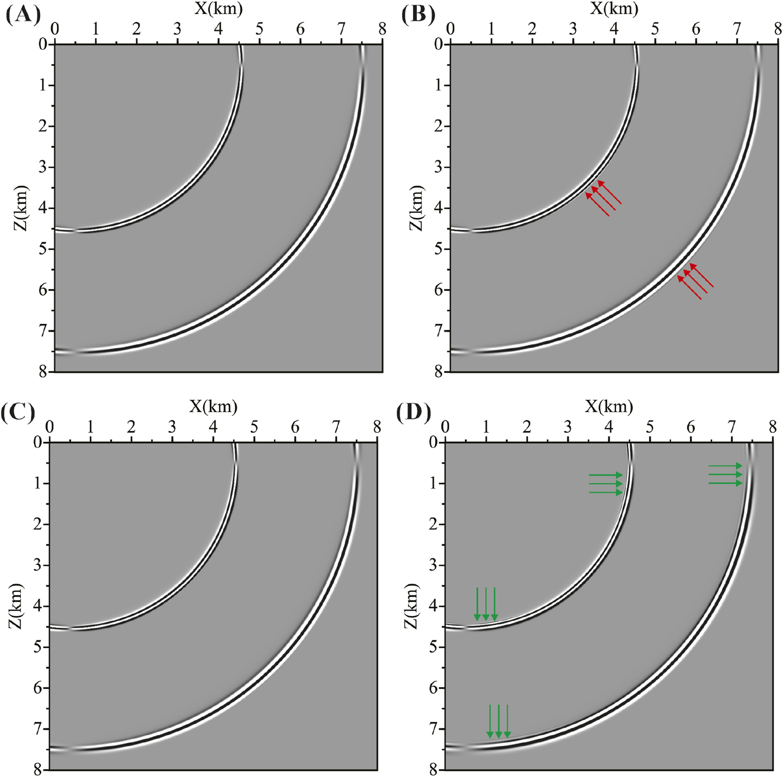
Wavefield snapshots of the component at 2.1 s simulated by C-SFD and TS-SFD for a homogeneous model. (A) Snapshot without numerical dispersion simulated by C-SFD with a very small temporal sampling interval serving as the reference solution. (B–D) Snapshots simulated by TS-SFD solving the decoupled P- and S-wave elastic wave equations by taking for calculating the difference coefficients based on the time–space domain P- and S-wave dispersion relations, respectively.
To analyze the influence of the value of , which is taken for calculating the difference coefficients of TS-SFD based on the time–space domain P- and S-wave dispersion relation, on the modeling accuracy, Figure 5A presents the snapshot without numerical dispersion simulated by C-SFD with a very small temporal sampling , which serves as the reference solution. Figures 5B–D presents the snapshots simulated by TS-SFD , with solving the decoupled P- and S-wave elastic wave equation by taking , respectively, for calculating the difference coefficients based on the time–space domain P- and S-wave dispersion relation. Comparing the snapshots simulated by TS-SFD with the reference solution, it can be observed that when taking , both P- and S-wave show slight temporal numerical dispersion, as illustrated by the red arrows in Figure 5B; when taking , both P- and S-waves show no visible numerical dispersion. When taking , both P- and S-wave show slight spatial numerical dispersion, as illustrated by the green arrows in Figure 5D.
The above analysis demonstrates that taking for calculating the difference coefficients of TS-SFD based on the time–space domain P- and S-wave dispersion relations can ensure that P- and S-waves achieve relatively high modeling accuracy, which is consistent with the conclusion drawn from the numerical dispersion based on Figure 2.
5.2 Layer model
Figure 6 provides a layer model. The model size is , with the spatial sampling interval , and thus, the grid number is . Figure 7 provides the wavefield snapshots of the component at 2.4 s simulated by C-SFD and TS-SFD , with for the layer model presented in Figure 6. In the simulations, a horizontally oriented force function characterized by a Ricker wavelet with a dominant frequency of 20 Hz located at (0.5 km, 0.5 km) is used as the source wavelet. Figure 8 presents the single-trace waveform at and extracted from the unseparated elastic wavefield snapshots of the component presented in Figure 7.
FIGURE 6

Layer model. (A) P-wave velocity model; (B) S-wave velocity model.
FIGURE 7

Wavefield snapshots of the component at 2.4 s simulated by C-SFD and TS-SFD for the layer model shown in Figure 6. Left: unseparated elastic wave wavefield snapshots; middle: separated P-wave wavefield snapshots; right: separated S-wave wavefield snapshots. (A) C-SFD . (B) TS-SFD , with the difference coefficients calculated based on the time–space domain P-wave dispersion relation. (C) TS-SFD , with the difference coefficients calculated based on the time–space domain S-wave dispersion relation. (D) TS-SFD solving the decoupled P- and S-wave elastic wave equation, in which the difference coefficients for solving the decoupled P- and S-wave equations are calculated based on the time–space domain P- and S-wave dispersion relations, respectively.
FIGURE 8

Single-trace waveform at (A) and (B) extracted from the unseparated elastic wavefield snapshots of the component shown in Figure 7, in which the blue curve serving as the reference solution is simulated by C-SFD , with a very small temporal sampling interval , and the red curves represent the simulated waveforms.① C-SFD ; ② TS-SFD , with the difference coefficients calculated based on the time–space domain P-wave dispersion relation; ③ TS-SFD , with the difference coefficients calculated based on the time–space domain S-wave dispersion relation; ④ TS-SFD solving the decoupled P- and S-wave elastic wave equations, in which the difference coefficients for solving the decoupled P- and S-wave equation are calculated based on the time–space domain P- and S-wave dispersion relation, respectively.
From Figures 7, 8, it can be observed that in the wavefield snapshots simulated by C-SFD , both P- and S-waves show obvious temporal numerical dispersion; in the wavefield snapshots simulated by TS-SFD , with the difference coefficients calculated based on the time–space domain P-wave dispersion relation, P-wave shows no visible numerical dispersion, but S-wave shows obvious spatial dispersion; in the wavefield snapshots simulated by TS-SFD with the difference coefficients calculated based on the time–space domain S-wave dispersion relation, S-wave shows no visible numerical dispersion, but P-wave shows some temporal numerical dispersion; and in the wavefield snapshots simulated by TS-SFD solving the decoupled P- and S-wave elastic wave equations, in which the difference coefficients for the decoupled P- and S-wave equation are calculated based on the time–space domain P- and S-wave dispersion relation, respectively, both P-wave and S-wave show no visible numerical dispersion.
The above layer model numerical simulation example demonstrates that directly using TS-SFD to solve the velocity–stress elastic wave equation, in which the P and S-waves are coupled together, irrespective of the difference coefficients calculated based on the time–space domain P- or S-wave dispersion relation, cannot ensure that both P- and S-waves reach relatively high modeling accuracy; performing elastic wave simulation by TS-SFD solving the decoupled P- and S-wave elastic wave equations, with the difference coefficients for solving the decoupled P- and S-wave equations calculated based on the time–space domain P- and S-wave dispersion relations, respectively, can ensure that both P- and S-waves achieve relatively high modeling accuracy. This conclusion is consistent with that drawn from the numerical dispersion based on Figure 3.
5.3 Tectonic-reservoir model from the Sichuan basin
Figure 9 presents a tectonic-reservoir model from the Sichuan basin. The model size is , with the spatial sampling interval , and thus, the grid number is . To perform elastic wave numerical simulation for this model with C-SFD and TS-SFD with an temporal sampling interval , an explosion source characterized by a Ricker wavelet, with a dominant frequency of 20 Hz located at (0.5 km, 0.5 km), is used. In the numerical simulation, C-SFD directly solves the velocity–stress elastic wave equation, and TS-SFD solves the decoupled P- and S-wave elastic wave equations, with the difference coefficients for solving the decoupled P- and S-wave equation calculated based on the time–space domain P- and S-wave dispersion relations, respectively.
FIGURE 9

Tectonic-reservoir model from the Sichuan basin. (A) P-wave velocity model; (B) S-wave velocity model.
Figure 10 presents the seismic record of the component simulated by TS-SFD . It shows that TS-SFD performs elastic wave simulation by solving the decoupled P- and S-wave elastic wave equation, thereby automatically and effectively separating the P- and S-waves. In addition, as an explosion source is used, the P-wave energy is dominant in the seismic record, and the S-wave of low energy belongs mainly to the converted wave.
FIGURE 10

Seismic record of the component simulated by TS-SFD solving the decoupled P- and S-wave elastic wave equations for the tectonic-reservoir model from the Sichuan basin presented in Figure 9. (A) Unseparated seismic record. (B) Separated P-wave seismic record. (C) Separated S-wave seismic record.
Figure 11 presents the 1000th trace waveform of the unseparated component simulated by C-SFD and TS-SFD . It shows that the waveform simulated by C-SFD exhibits a marked discrepancy from the reference waveform, indicating that both the P- and S-waves simulated by C-SFD have significant numerical dispersion, while the waveform simulated by TS-SFD (M = 8) exhibits a high degree of coincidence with the reference waveform, suggesting that the P- and S-waves simulated by TS-SFD have no visible numerical dispersion.
FIGURE 11

The 1000th trace waveform of the unseparated component simulated by C-SFD and TS-SFD for the tectonic-reservoir model from the Sichuan basin presented in Figure 9, in which the blue curve serving as the reference solution is simulated by C-SFD (M = 20), with a very small temporal sampling , and the red curves represent the simulated waveforms.① C-SFD , ② TS-SFD solving the decoupled P- and S-wave elastic wave equation, in which the difference coefficients for solving the decoupled P- and S-wave equation are calculated based on the time–space domain P- and S-wave dispersion relations, respectively. (A) Time range 1.5–3.0 s, in which the reflected P-wave dominates; (B) time range 3.0–4.5 s, in which the converted S-wave dominates.
Numerical simulation examples on this tectonic-reservoir model from the Sichuan basin further demonstrate that performing elastic wave numerical simulation with TS-SFD by solving the decoupled P- and S-wave elastic wave equation, with the difference coefficients for solving the decoupled P- and S-wave equation calculated based on the time–space domain P- and S-wave dispersion relations, respectively, can ensure that both P- and S-waves achieve relatively high modeling accuracy and can automatically and effectively separate the P- and S-waves. Moreover, this example also demonstrates that this simulation strategy has good applicability to complex models.
6 Conclusion
In this article, we propose a novel strategy to perform elastic wave numerical simulation. This strategy is characterized by TS-SFD solving the decoupled P- and S-wave elastic wave equations, with the difference coefficients for solving the decoupled P- and S-wave equations calculated based on the time–space domain P- and S-wave dispersion relations, respectively. Through the numerical dispersion analysis, stability analysis, and numerical simulation experiments, the following conclusions can be drawn:
When calculating the difference coefficients for TS-SFD based on the time–space domain P- and S-wave dispersion relations, the differential coefficients are related to the value of , and taking can ensure that P- and S-waves achieve relatively high modeling accuracy.
Numerical dispersion analysis and stability analysis demonstrate that the novel strategy proposed in this article can not only ensure that both P- and S-waves achieve relatively high modeling accuracy but also improve the numerical stability.
Numerical simulation experiments demonstrate that the novel strategy proposed in this paper can ensure that both P- and S-waves achieve relatively high modeling accuracy and can automatically and effectively separate the P- and S-waves. Moreover, this strategy has good applicability to complex models.
Despite the distinct advantages offered by the elastic wave numerical simulation method proposed in this article, there are several limitations that require further investigation and resolution:
The algorithm for calculating the difference coefficients of TS-SFD is derived based on square grids. A variant of TS-SFD that can be used with rectangular grids should be developed to extend its range of applications.
The method described in this article is applicable solely to isotropic elastic wave equations; further development may be pursued to establish simulation techniques suitable for anisotropic elastic wave equations.
Statements
Data availability statement
The original contributions presented in the study are included in the article/supplementary material, further inquiries can be directed to the corresponding author.
Author contributions
XS: Methodology, Visualization, Writing – original draft. CW: Conceptualization, Formal analysis, Resources, Writing – review and editing. WL: Investigation, Methodology, Validation, Writing – review and editing. DZ: Data curation, Software, Supervision, Writing – review and editing. ZH: Conceptualization, Data curation, Formal analysis, Investigation, Writing – original draft. YF: Investigation, Project administration, Validation, Visualization, Writing – review and editing. YG: Investigation, Methodology, Resources, Supervision, Writing – review and editing. ZZ: Conceptualization, Data curation, Resources, Supervision, Writing – original draft.
Funding
The author(s) declared that financial support was not received for this work and/or its publication.
Conflict of interest
Authors XS, CW, DZ, YF, YG, and ZZ were employed by Shale Gas Research Institute, PetroChina Southwest Oil & Gas Field Company.
Authors CW and YG were employed by BGP Inc., China National Petroleum Corporation.
The remaining author(s) declared that this work was conducted in the absence of any commercial or financial relationships that could be construed as a potential conflict of interest.
Generative AI statement
The author(s) declared that generative AI was not used in the creation of this manuscript.
Any alternative text (alt text) provided alongside figures in this article has been generated by Frontiers with the support of artificial intelligence and reasonable efforts have been made to ensure accuracy, including review by the authors wherever possible. If you identify any issues, please contact us.
Publisher’s note
All claims expressed in this article are solely those of the authors and do not necessarily represent those of their affiliated organizations, or those of the publisher, the editors and the reviewers. Any product that may be evaluated in this article, or claim that may be made by its manufacturer, is not guaranteed or endorsed by the publisher.
References
1
Alterman Z. Karal F. C. (1968). Propagation of elastic waves in layered media by finite difference methods. Bull. Seismol. Soc. Am.58, 367–398.
2
Cao J. Chen J.-B. (2018). A parameter-modified method for implementing surface topography in elastic-wave finite-difference modeling. Geophysics83, T313–T332. 10.1190/geo2018-0098.1
3
Chen H. Zhou H. Zhang Q. Chen Y. (2017). Modeling elastic wave propagation using k-space operator-based temporal high-order staggered-grid finite-difference method. IEEE Trans. Geoscience Remote Sens.55, 801–815. 10.1109/TGRS.2016.2615330
4
Dong L. Ma Z. Cao J. Wang H. Geng J. Bing L. et al (2000). A staggered-grid high-order difference method of one-order elastic wave equation (in Chinese). Chin. J. Geophys.43, 411–419.
5
Du Q. Zhu Y. Ba J. (2012). Polarity reversal correction for elastic reverse time migration. Geophysics77, S31–S41. 10.1190/geo2011-0348.1
6
Du Q. Gong X. Zhang M. Zhu Y. Fang G. (2014). 3d ps-wave imaging with elastic reverse-time migration. Geophysics79, S173–S184. 10.1190/geo2013-0253.1
7
Graves R. W. (1996). Simulating seismic wave propagation in 3d elastic media using staggered-grid finite differences. Bull. Seismol. Soc. Am.86, 1091–1106. 10.1785/bssa0860041091
8
Kane Y. (1966). Numerical solution of initial boundary value problems involving maxwell’s equations in isotropic media. IEEE Trans. Antennas Propag.14, 302–307. 10.1109/TAP.1966.1138693
9
Levander A. R. (1988). Fourth-order finite-difference p-sv seismograms. Geophysics53, 1425–1436. 10.1190/1.1442422
10
Li Z. Zhang H. Liu Q. Han W. (2007). Numerical simulation of elastic wavefield separation by staggering grid high-order finite-difference algorithm (in Chinese). Oil Geophys. Prospect.42, 510–515.
11
Liu Y. Sen M. K. (2011). Scalar wave equation modeling with time–space domain dispersion-relation-based staggered-grid finite-difference schemes. Bull. Seismol. Soc. Am.101, 141–159. 10.1785/0120100041
12
Ma D. Zhu G. (2003). Numerical modeling of p-wave and s-wave separation in elastic wavefield (in Chinese). Oil Geophys. Prospect.38, 482–486.
13
Peng G. Liu W. Guo N. Hu Z. Xu K. Pei G. (2022). A time-space domain dispersion-relationship-based staggered-grid finite-difference scheme for modeling the stress-velocity acoustic wave equation (in Chinese). Geophys. Prospect. Petroleum61, 156–165. 10.3969/j.issn.1000-1441.2022.01.016
14
Ren Z. Li Z. C. (2017). Temporal high-order staggered-grid finite-difference schemes for elastic wave propagation. Geophysics82, T207–T224. 10.1190/geo2017-0005.1
15
Ren Z. Liu Y. (2015). Acoustic and elastic modeling by optimal time-space-domain staggered-grid finite-difference schemes. Geophysics80, T17–T40. 10.1190/geo2014-0269.1
16
Singh S. Tsvankin I. Naeini E. Z. (2018). Bayesian framework for elastic full-waveform inversion with facies information. Lead. Edge37, 924–931. 10.1190/tle37120924.1
17
Su Z. Trad D. (2018). Elastic modeling and reverse time migration. CREWES Res. Rep.30.
18
Sun R. McMechan G. A. Hsiao H.-H. Chow J. (2004). Separating p- and s-waves in prestack 3d elastic seismograms using divergence and curl. Geophysics69, 286–297. 10.1190/1.1649396
19
Tan S. Huang L. (2014). An efficient finite-difference method with high-order accuracy in both time and space domains for modelling scalar-wave propagation. Geophys. J. Int.197, 1250–1267. 10.1093/gji/ggu077
20
Virieux J. (1984). Sh-wave propagation in heterogeneous media: velocity-stress finite-difference method. Geophysics49, 1933–1942. 10.1190/1.1441605
21
Virieux J. (1986). P-sv wave propagation in heterogeneous media: velocity-stress finite-difference method. Geophysics51, 889–901. 10.1190/1.1442147
22
Virieux J. Operto S. (2009). An overview of full-waveform inversion in exploration geophysics. Geophysics74, WCC1–WCC26. 10.1190/1.3238367
23
Wang W. McMechan G. A. Zhang Q. (2015). Comparison of two algorithms for isotropic elastic p and s vector decomposition. Geophysics80, T147–T160. 10.1190/geo2014-0563.1
24
Wang H. He B. Shao X. (2022). Numerical simulation of first-order velocity-dilatation-rotation elastic wave equation with staggered grid (in Chinese). Oil Geophys. Prospect.57, 1352–1361. 10.13810/j.cnki.issn.1000-7210.2022.06.010
25
Wang M. Li Y. Chen Y. Fu Z. Wang D. Tang F. (2025). An average-derivative based second-order staggered-grid finite-difference scheme for 3d frequency-domain elastic wave modeling. Geophysics90, T79–T97. 10.1190/geo2024-0574.1
26
Wu X. Liu Y. Cai X. (2018). Elastic wavefield separation methods and their applications in reverse time migration (in Chinese). Oil Geophys. Prospect.53, 710–721. 10.13810/j.cnki.issn.1000-7210.2018.04.007
27
Zhou H. Liu Y. Wang J. (2022). Elastic wave modeling with high-order temporal and spatial accuracies by a selectively modified and linearly optimized staggered-grid finite-difference scheme. IEEE Trans. Geoscience Remote Sens.60, 1–22. 10.1109/TGRS.2021.3078626
28
Zhou H. Zhang L. Zhang Y. (2024). Simulation of scalar wave propagation with high-order temporal and spatial accuracy by a new multi-axial staggered-grid finite-difference scheme. Bull. Seismol. Soc. Am.115, 1–21. 10.1785/0120240148
29
Zhu H. (2017). Elastic wavefield separation based on the helmholtz decomposition. Geophysics82, S173–S183. 10.1190/geo2016-0419.1
Summary
Keywords
elastic wave, numerical modeling, numerical dispersion, time–space domain, difference-coefficient calculation
Citation
Shi X, Wang C, Liu W, Zhang D, Hu Z, Feng Y, Gao Y and Zhou Z (2026) Elastic-wave-equation numerical simulation using a time–space domain dispersion-relation-based staggered-grid finite-difference method. Front. Earth Sci. 13:1675515. doi: 10.3389/feart.2025.1675515
Received
29 July 2025
Revised
31 October 2025
Accepted
30 November 2025
Published
06 January 2026
Volume
13 - 2025
Edited by
Yong Zheng, China University of Geosciences Wuhan, China
Reviewed by
Adil Ozdemir, Georesources and Geoenergy, Türkiye
Hongyu Zhou, China University of Geosciences Wuhan, China
Updates
Copyright
© 2026 Shi, Wang, Liu, Zhang, Hu, Feng, Gao and Zhou.
This is an open-access article distributed under the terms of the Creative Commons Attribution License (CC BY). The use, distribution or reproduction in other forums is permitted, provided the original author(s) and the copyright owner(s) are credited and that the original publication in this journal is cited, in accordance with accepted academic practice. No use, distribution or reproduction is permitted which does not comply with these terms.
*Correspondence: Wei Liu, liuwei2013@petrochina.com.cn
Disclaimer
All claims expressed in this article are solely those of the authors and do not necessarily represent those of their affiliated organizations, or those of the publisher, the editors and the reviewers. Any product that may be evaluated in this article or claim that may be made by its manufacturer is not guaranteed or endorsed by the publisher.