Efficient vegetation filtering method using K-means clustering algorithm: case study of high steep rock slope

Vegetation obscures critical rock-mass features on steep slopes, degrading the reliability of structural surface interpretation from point clouds. We propose a fast vegetation-filtering approach tailored to high-steep, vegetated rock slopes. The method aims to suppress vegetation noise while preserving terrain points essential for structural analysis. We first perform dual-channel dimensionality reduction by combining Principal Component Analysis (PCA) on spatial coordinates with the Red–Green Difference Index (RGDI) from RGB values, then apply K-means clustering for segmentation. A hierarchical grid plus local plane fitting is used to select vegetation seed points; distances to the fitted plane guide seed assignment and subsequent cluster-level filtering. To prevent over-filtering, a preservation mechanism based on the 3σ rule retains 5%–32% of points near the seed-point distance threshold. The method was evaluated on a rugged, vegetation-covered slope at Tiantai Mountain (Zhejiang, China) acquired with a Topcon GLS-2000 (384,663 points). The effectiveness of the filtering results is evaluated using class error, I_e, II_e and total error A_e. Comparing with other algorithms, it is found that the class error, I_e is 7.79%, the class error II_e is 4.34%, and the total result is limited to 6.53%. By jointly leveraging spatial and spectral cues with grid-wise plane fitting and a preservation guarantee, the approach effectively suppresses vegetation noise while retaining terrain detail needed for downstream tasks (e.g., structural plane interpretation). The results indicate improved filtering accuracy and robustness for high-steep terrains relative to traditional methods.

1 Introduction

Rocky high steep slopes are among the most dangerous disaster-causing geological bodies in large-scale engineering projects, like water conservancy and hydropower projects, railway tunnels, and metal mines, and so on. The internal stability of some of these slopes is poor and poses safety hazard, such as landslides and mudslides (Zheng et al., 2021; Zheng et al., 2024), posing threats not only to the lives of local residents and construction workers but also impeding geological investigation (Zhao et al., 2023) and surveying efforts (Jia et al., 2018). The stability of the rock mass is governed by its characteristics, making it crucial to acquire detailed information about the surface structure of the rocks in order to accurately understand the stability of high steep slopes.

In particular, the selected study area features complex geological conditions, steep terrain, and dense vegetation coverage, which pose significant challenges to traditional field-based structural interpretation. These characteristics make it a representative case for testing automated filtering and structural plane (Zhou et al., 2024) recognition methods in real-world slope environments.

However, the traditional approaches of obtaining information typically rely on field measurements by geological survey personnel, requiring pre-formulated survey routes. This approach has several drawbacks, including the difficulty of predicting on-site risks, significant manpower and time consumption. The integration of three-dimensional laser scanning and Unmanned Aerial Vehicle (UAV) technology offers a flexible solution for rapidly and accurately acquiring crucial surface data of geological structures. However, the presence of extensive vegetation cover (Tingting et al., 2023) on the rock surface often obscures ground points, resulting in their omission from the actual results. Effectively separating vegetation noise points while preserving fundamental rock structure characteristics, and simultaneously ensuring the retention of ground points, represents a pressing challenge in current research.

Point cloud filtering is typically the first step in point cloud processing, aimed at addressing irregularities in point cloud density, noise effects, and the presence of discrete points that require processing due to occlusion. Currently, there are various methods available for filtering point cloud data. These methods can be broadly categorized as follows: the digital morphology-based filtering algorithm, the terrain slope-based filtering algorithm, the surface fitting-based filtering algorithm, interpolation-based filtering algorithms, as well as certain segmentation and clustering algorithms tailored for three-dimensional point cloud data processing. The digital morphology-based filtering algorithm was first introduced in 1993. It belongs to a class of nonlinear filtering methods (Giuseppe, 2023; Nie et al., 2017) developed based on digital morphology principles. Its morphological transformations mainly involve corrosion, expansion, open operation, and closed operation, which facilitate the discrimination between ground and non-ground points. While this algorithm is relatively straightforward and user-friendly, allowing for better preservation of intricate details in the original image, it faces challenges in handling undulating terrains or sudden, drastic changes. Additionally, it is susceptible to the influence of window size. The terrain slope-based filtering algorithm (Wan et al., 2018; Susaki, 2012) assesses the height difference between two points by comparing it to a specific threshold value derived from a priori knowledge estimation or manual training. This process enables the algorithm to make trade-offs and determine the characteristics of the points. However, the accuracy of this algorithm’s assessment decreases in areas with significant terrain slope undulations or fracture conditions. The surface fitting-based filtering algorithm (Xing et al., 2017; Li et al., 2016; Mongus et al., 2012) utilizes data fitting models to create a local surface element that approximates actual terrain features. By comparing the distances between neighboring points and the surface against predefined value, it iteratively refines and reorganizes until the optimal solution is achieved. This algorithm has broader applications and operates at higher speeds, but selecting an appropriate window size poses challenge. Interpolation-based filtering algorithms primarily include the algorithm based on irregular triangular mesh (Błaszczak-Bąk et al., 2011; Zhang and Lin, 2013a) and the linear prediction method (Mikita et al., 2013). The operation process of these algorithms is relatively straightforward, with a clear and simple core concept. However, the iterative cascading process can potentially accumulate errors in the outcome.

Furthermore, in the field of rock engineering, several intelligent algorithms are widely utilized for processing three-dimensional point cloud data. These algorithms encompass clustering algorithms, region growth methods, and the Hough transform method. In this context, clustering algorithms play a pivotal role in the intelligent processing of point cloud data, particularly in the identification of structural surface within rock formations. Among these, the clustering method based on normal vectors is widely employed. Notable examples include the C-means (Havens et al., 2012) and K-means clustering algorithms (Shi et al., 2024; Pugazhenthi and Kumar, 2020; Turkes, 2017; Xu, 2014; Chong, 2021; Tang et al., 2023; Mu et al., 2024). In this clustering algorithm, normal vectors serve as the fundamental data source for clustering, enabling the conversion of three-dimensional location information into two-dimensional location information that can measure normal vectors. Nevertheless, this approach may also lead to erroneous removal. The region growing method (Sihong et al., 2021; Jothiaruna et al., 2020; Yang and Zhai, 2019) initiates by manually or randomly selecting seed points. It then identifies points with similar attributes to the seed points in their vicinity and merges them into the region or set containing the seed points. This process continues iteratively until no remaining similar points are found, indicating the completion of region or set growth. However, this approach involves multiple neighborhood searches and iterations, which reduces the efficiency and poses challenges for swift three-dimensional target extraction. The Hough transform method is a fundamental technique for detecting geometric shapes in images. It achieves this by transforming the coordinate equations of points in point cloud data into polar coordinate space. Subsequently, a set corresponding to the particular shape is obtained through the Hough transform using techniques such as voting statistics and peak detection in polar coordinate space. Nonetheless, it is characterized by high computational complexity in both time and space, making it unsuitable for scenarios involving curved surface or irregular concave and convex surface.

As mentioned above, the traditional algorithm is characterized by a simple foundational theory but a complex frame structure. Consequently, this leads to excessively intricate logic cycles, thereby making the clustering algorithm within the three-dimensional intelligent algorithm more suitable for filtering vegetation point clouds. This method has the advantages of fast speed, good segmentation effect and strong adaptability. Additionally, the reduction of location information dimensionality plays a crucial role as it effectively alleviates the complexity level of the algorithm.

Although previous studies have proposed various filtering and classification techniques, many of these approaches are designed for urban environments or moderately sloped terrain. Their applicability to steep, vegetation-covered rock slopes remains limited, especially in preserving critical geological features while removing surface vegetation noise. This study addresses this gap by introducing a dual-channel dimensionality reduction technique and an unsupervised clustering strategy tailored specifically for high-steep terrain, aiming to improve both filtering accuracy and structural feature retention.

This paper conducts a comparative study of existing algorithm and identifies areas for improvement in the proposed method. The new algorithm primarily utilizes Principal Component Analysis (PCA) to reduce the dimensionality of pre-processed original point cloud data. Subsequently, it applies the K-means clustering algorithm to analyze the point cloud data and address the aforementioned issues. This combined approach not only outperforms traditional methods in handling specific issues such as noise, but also addresses the limitations of existing methods in certain application scenarios, demonstrating strong adaptability and effectiveness.

The study is structured as follows: Firstly, it outlines the overall algorithmic process, providing detailed elaboration. Next, it describes the data selection for experiments and the methods employed for error evaluation. The results are analyzed both in a general sense and concerning discrete-value sensitivity. Finally, the effectiveness of the new algorithm in this paper is assessed through a comparison with other algorithms.

In light of the above, this study proposes an improved vegetation filtering method specifically designed for high-steep, vegetated rock slopes. By integrating Principal Component Analysis (PCA) and the Red-Green Difference Index (RGDI) for dual-channel dimensionality reduction, and applying K-means clustering to segment feature points, the method aims to enhance filtering accuracy and structural information preservation. The effectiveness of the proposed approach is evaluated through comparative experiments on a 3D-printed model derived from real geological data.

2 Materials and methods

The algorithm presented in this paper is based on the utilization of Principal Component Analysis (PCA) and the Red-Green Difference Index (RGDI) to reduce the dimensionality of the original point cloud data. Subsequently, the K-means clustering technique is applied to cluster the data. Following that, vegetation seed points are identified by analyzing the differences in point cloud morphology distribution between rocks and vegetation. These identified seed points are then integrated with the clustering outcomes and the selection of vegetation noise points. In this section, we will describe six key aspects of the algorithm: the overall procedure, principal component analysis, K-means clustering algorithm and vegetation noise points filtering, point cloud data gridding, seed point and noise point selection, and preservation guarantee settings.

2.1 Overall procedure

The algorithm is executed in the following steps: Firstly, a regular grid is established. Secondly, Principal Component Analysis (PCA) is applied to reduce the dimensionality of the positional information $\left(x,y,z\right)$ in the original point cloud data. The first column of data after dimensionality reduction was selected to be combined with the red-green difference index at each point, a two-dimensional dataset is created, encompassing both positional and RGB color information for each point. Subsequently, the K-means algorithm is employed on this two-dimensional point cloud data. Then, leveraging slope information from the SPF algorithm (Yan et al., 2021) and incorporating the concept of plane fitting, each grid is divided into a two-tiered grid to select the lowest points. The four lowest points are fitted to a plane using the least squares method. The distance from each point in the grid to the fitting plane is calculated, and the point with the largest distance is selected. It is then determined whether the point belongs to the ground. If it is classified as a non-ground point, it is chosen as a vegetation seed point. Based on the cluster number of the vegetation seed point obtained from the cluster analysis, all points belonging to the same cluster within the grid are identified as non-ground points. These steps are repeated until the data in the grid meet the required criteria. The flowchart of the algorithm is illustrated in Figure 1.

Figure 1

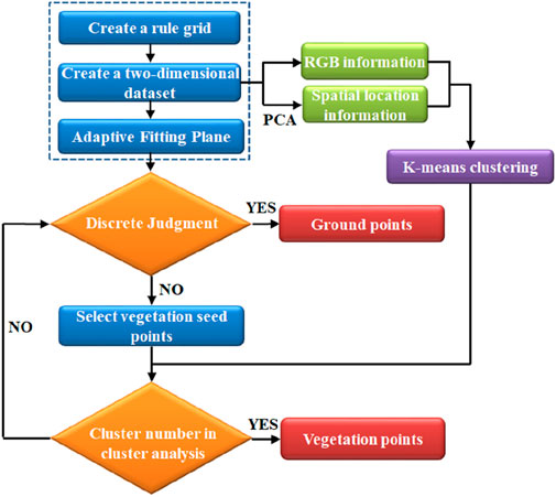
Figure 1. Flowchart of a vegetation filtering algorithm using K-means clustering.

The integration of spatial information and color information for dual-factor filtering aims to address the limitation of relying solely on the red-green difference index, which provides a single basis for judgment. This approach is designed to preserve as much vegetation-related point cloud data as possible that reflects the surface morphology of the rock mass. By doing so, subsequent point cloud processing tasks—such as the generation of digital surface models (DSM) and the intelligent identification of structural planes—can better reflect real-world geological conditions.

2.2 Principal component analysis

PCA is a statistical method widely used in dimensional reduction in mathematics and has extensive practical applications. It is employed in various disciplines, including demography, quantitative geography, molecular dynamics simulation, mathematical modeling, and mathematical analysis. It is a frequently utilized tool for multivariate analysis (Lin and Du, 2013).

In the context of processing point cloud data in rock engineering, the PCA method can be applied to transform linearly uncorrelated location information $\left(x,y,z\right)$. Then, based on the fact that the first principal component reflects the largest difference in the group of data, the algorithm in this chapter selects the first principal component as one of the data sources for the subsequent calculations.

The process of conducting principal component analysis on the location information $\left(x,y,z\right)$ of point cloud data involves the following steps:

First, the three-dimensional raw position information data $X=x,y,z=\left(x_1{,x}_2,x_3\right)$, which consists of ‘n' point cloud data, is subjected to normalization. Equation 1 used for this purpose is as follows:

$Z_{ij}=\frac{x_{ij}-\overline{x_j}}{\sqrt{s_j}},i=1,2,\dots ,n;j=1,2,3(1)$

Among them, $\overline{x_j}=\frac{{\sum }_{i=1}^n{x}_{ij}}{n}$ and $s_j^2=\frac{{\sum }_{i=1}^n{\left(x_{ij}-\overline{x_j}\right)}^2}{n-1}$, and obtain the normalization matrix Z from the above equation.

Then, a matrix of correlation coefficients needs to be obtained. The following Equation 2 is used:

$R={\left[r_{ij}\right]}_p{x}_p=\frac{Z^{T}Z}{n-1}(2)$

Among them, $r_{ij}=\frac{{\sum }_{t=1}^n{x}_{ti}{x}_{tj}}{n-1}\left(i,j=1,2,3\right)$, and find the correlation coefficient matrix R according to the above equation.

Finally, the eigenvalues ${\lambda }_j$ and the corresponding eigenvectors $b_j$ of the correlation coefficient matrix R are solved using the characteristic equation $\left|R-\lambda I_p\right|=0$. And the standardized indicator variables were transformed into principal components using Equation 3:

$U_{ij}=z_i^T{b}_j(3)$

Where $z_i$ is the ith row of the normalization matrix. The resulting principal component matrices $U=\left(U_1,U_2,U_3\right)$, $U_1$ are denoted as the first principal component, $U_2$ as the second principal component and $U_3$ as the third principal component. In general, $U_1$, the largest of all linear combinations, is selected instead of the location information $\left(x,y,z\right)$ as the basis for subsequent calculations. In other words, $U_1$ is obtained by dimensionality reduction of the location information using principal component analysis.

2.3 K-means clustering algorithm and vegetation noise points filtering

2.3.1 Theoretical background of K-means clustering in rock engineering

Clustering is an unsupervised learning technique that organizes data points into groups based on their similarity. Among various clustering algorithms, K-means clustering is widely adopted due to its simplicity and computational efficiency. The basic principle involves partitioning a dataset into K clusters by minimizing the intra-cluster variance. The algorithm begins by randomly selecting K initial centroids, assigning each data point to the nearest centroid based on a chosen distance metric, and iteratively updating the centroids until convergence. The termination criteria may include minimal changes in cluster membership, minimal shifts in centroids, or minimization of the total intra-cluster distance (Sud et al., 2020).

In rock engineering, geological structural planes—formed through processes such as sedimentation, tectonic activity, and weathering—introduce spatial discontinuities, inhomogeneities, and anisotropies within the rock mass. These discontinuities significantly affect the mechanical behavior and failure mechanisms of rock slopes. Therefore, accurate extraction of structural planes from point cloud data is of critical importance. K-means clustering, due to its robust partitioning capabilities, provides a practical and effective approach for classifying spatial features in rock-mass datasets.

2.3.2 Implementation of K-means clustering for vegetation noise filtering

In this study, K-means clustering is employed to filter vegetation noise points from the point cloud data. The raw data, consisting of six-dimensional vectors $\left(x,y,z,r,g,b\right)$ is transformed into a two-dimensional feature space $\left(X_1,X_2\right)$ through a dual-channel approach. Specifically, Principal Component Analysis (PCA) is applied to spatial coordinates to derive X₁, capturing major orientation trends, while the Red-Green Difference Index (RGDI) is computed from RGB values to form X₂, enhancing vegetation color contrast. The K-means clustering is implemented as shown in Equation 4:

$\left[idx,C,sumd,D\right]=km\mathrm{e}ans\left(X,K\right)(4)$

In this study, the number of clusters K for the K-means algorithm was empirically set to 6, which aligns with the expected classification of surface features into categories such as low vegetation, high vegetation, bare rock, and noise. The choice of K = 6was guided by preliminary tests and prior studies, which demonstrated that clustering with 5 ≤ K ≤ 8typically yields stable results in vegetation filtering tasks involving spatial and spectral features of point clouds. Xu et al. (Simoniello et al., 2022) and Zhang et al. (Chen et al., 2024) both employed similar clustering scales in their segmentation of vegetated terrain, and their results support the efficacy of this cluster number in balancing classification granularity and computational efficiency.

In this context, $K$ represents the number of classes into which the original data set is divided and must be an integer; $X=\left(X_1,X_2\right)$, $X_1$ represents the location information reduced to one-dimensional data by PCA; $X_2$ denotes the RGDI of RGB color information; $i dx$ is a vector that stores the cluster labels of the point clusters to which each point cloud data belongs after clustering analysis of the original data set. $C$ is a matrix that stores the cluster center coordinates of the ‘K’ point clusters, in this algorithm a matrix of K rows and two columns; $sumd$ is a vector that stores the sum of the distances of all points within a point cluster to the cluster center of the corresponding point cluster; $D$ is the matrix that stores the distance of each point to the cluster center of all point clusters respectively.

2.4 Point cloud data gridding

The original point cloud data lacks topological connectivity relationships and associated structural information, which makes it disorganized and difficult to process. Therefore, after obtaining the point cloud data information using a three-dimensional laser scanner, the initial step is to generate a regular grid to mesh the raw point cloud data to homogenize the point cloud data.

Gridding is a commonly used method for processing point cloud data. In simple terms, it involves placing the point cloud data into a pre-divided regular grid. This allows for later processing, where the grid is treated as a unit for tasks such as chunking or semantic segmentation. Gridding is typically performed in either two or three dimensions. In this algorithm, a square grid is employed to create a two-dimensional grid surface. The grid is divided without considering other information except $\left(x,y\right)$. In order to avoid excessive computation, the grid spacing is determined according to the density of the point cloud, and the point cloud data is now divided into first level of grid. Figure 2a illustrates the results of the first-level gridding of a set of point cloud data.

Figure 2

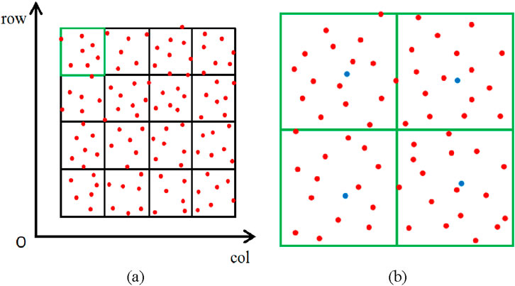
Figure 2. Point cloud data gridding. (a) First-level gridding: The original point cloud is partitioned into coarse grid cells based on the spatial extent. Each red dot represents a point within the 3D point cloud. (b) Second-level gridding: Each first-level cell is further subdivided into finer sub-grids to enhance local plane fitting accuracy. Blue dots indicate points selected for local surface fitting in each sub-grid.

After partitioning the first-level grid, the second-level grid is subdivision to achieve the highest accuracy in fitting the ground plane. The procedure begins by dividing the first-level grid into four blocks, resulting in the creation of a new second-level grid. The lowest point within each second-level grid is then identified as the seed point for the ground by z-coordinate, as shown by the blue dots in Figure 2b. The grid division lines are defined by Equations 5, 6:

$X_z=\frac{x_{{\mathit{max}}^{\prime }}+x_{{\mathit{min}}^{\prime }}}{2}(5)$

$Y_z=\frac{y_{{\mathit{max}}^{\prime }}+y_{{\mathit{min}}^{\prime }}}{2}(6)$

The grid resolution in the first-level gridding was set to 0.1 m, which corresponds to approximately twice the average point spacing of the input dataset. This choice ensures sufficient granularity for local surface fitting while maintaining computational efficiency. Similar grid resolutions have been applied in terrain filtering tasks for airborne and terrestrial LiDAR data. A coarser grid size would risk missing finer structural details, while overly fine grids increase the risk of overfitting and computational burden.

In this context, $X_z$ represents the $x$-coordinate of the vertical dividing line, while $Y_z$ denotes the $y$-coordinate of the horizontal dividing line. Additionally, ${x_{\mathit{max}}}^{\prime }$, ${y_{\mathit{max}}}^{\prime }$, ${x_{\mathit{min}}}^{\prime }$ and ${y_{\mathit{min}}}^{\prime }$ refer to the maximum and minimum values of $\left(x,y\right)$ within the point cloud data of the corresponding level grid. Figure 2b illustrates the outcomes obtained from the second-level gridding process applied to a set of point cloud data.

2.5 Seed point and noise point selecting

2.5.1 Theoretical background: seed point selection and plane fitting

In point cloud processing, identifying and eliminating vegetation noise is crucial for the accurate extraction of terrain features. A common approach involves selecting seed points based on the geometric deviation of points from a locally fitted plane. The plane is typically computed using a least squares regression of selected sample points.

The local fitting plane is expressed by Equation 7:

$Z=aX+bY+c(7)$

The parameters $a$, $b$ and $c$ are calculated using the least squares method. Subsequently, the formula for determining the distance between each point in the primary grid and the corresponding fitting plane is given Equation 8:

$s_i=\frac{\left|a{x}_i+b{y}_i-z_i+c\right|}{\sqrt{a^2+b^2+1}}(8)$

The distance from each point in the traversal level grid to the fitting plane is denoted as $s_i$. The three-dimensional coordinates of each point in the grid are represented by $\left(x_i,y_i,z_i\right)$. The parameters $a$, $b$ and $c$ are determined using the least squares method.

Subsequently, the discretization of the distance can be obtained using the following Equation 9:

$STD=\sqrt{\frac{{\sum }_{i=1}^n{\left(x_i-\overline{x}\right)}^2}{n-1}}(9)$

Points that deviate significantly from the fitted plane may indicate the presence of vegetation or other outliers. Identifying such points allows for the designation of vegetation seed points, which can guide subsequent noise filtering.

2.5.2 Implementation of SPF-Based vegetation noise filtering in this study

In this study, a hierarchical grid-based method is employed for vegetation noise identification. The Surface Projection Fitting (SPF) algorithm is a local adaptive filtering technique that identifies vegetation by measuring point-wise deviations from a fitted terrain surface. It is particularly effective for steep, rugged slopes where elevation-based global filters may fail.

After establishing a second-level grid over the point cloud, the first step is to assess whether vegetation noise exists in the corresponding first-level grid. To aid in manual validation, CloudCompare software is used to visualize and remove obviously noise-free areas.

Following the Surface Projection Fitting (SPF) algorithm (Yang and Zhai, 2019), the four lowest points in each second-level grid are selected to construct a local plane using the least squares method. This approach has been experimentally proven to be effective in filtering low vegetation while preserving steep terrain, making it highly suitable for applications involving complex topography.

If vegetation noise is detected in a first-level grid, seed points are identified by selecting the point with the maximum vertical deviation from the fitted plane. This point is assigned as a vegetation seed point. Subsequent vegetation points are then identified and clustered based on their proximity to the seed point and shared cluster label in the earlier K-means segmentation stage.

This process ensures a focused removal of vegetation points while minimizing the risk of over-filtering terrain features essential for structural surface extraction.

2.6 Preservation guarantee settings

In this study, the preservation guarantee mechanism is inspired by the normal distribution. The introduced vegetation filtering algorithm utilizes PCA and K-means clustering algorithm. The retention threshold ρ, ranging from 5% to 32%, was selected based on the empirical 3σ rule from Gaussian distribution statistics, ensuring that the majority of terrain points (up to 95%) are preserved while excluding extreme outliers commonly representing vegetation. Similar percentile-based approaches have been adopted by Meng et al. (2010) in ground filtering algorithms. The specific interval was further validated by comparing the filtered outputs with manually labeled reference datasets to ensure optimal balance between terrain preservation and vegetation noise suppression.

Once the vegetation seed points are determined, the selection of vegetation noise points is based on the number of clusters to which the points belong after clustering and segmentation. After identifying the cluster containing the vegetation seed point, we apply the fundamental concept of the “68–95-99.7 rule” of normal distribution, commonly known as the “rule of thumb”. If a set of data conforms to this rule, 68% of the values falls within the first standard deviation, 95% within the second standard deviation, and 99.7% within the third standard deviation.

To prevent excessive filtering and considering the random distribution of the point cloud data, we introduce a parameter '$s_i$'. We establish a criterion: if the '$s_i$' value of a noise point, selected based on the cluster of points containing the vegetation seed points, is less than 5%–32% of the '$s_i$' value of the corresponding vegetation seed point, it is considered part of the rock mass point cloud data. These points are retained and included in the subsequent calculation cycle.

Due to the complexity of the rock mass engineering and the varying surface conditions of the rock masses to be collected, the point cloud data in the first-level grid tends to be more scattered compared to other grids. Therefore, it is crucial to implement a specific judgment mechanism to prevent excessive filtering. Since this paper focuses on low and medium-density vegetation areas, the point cloud data related to rock masses constitute a significant portion. Removing too many noise points at once can result in excessive filtering. Hence, it is essential to establish a percentage to prevent this scenario.

2.7 Data selection

This study focuses on point cloud data collected from a rugged and steep slope located within Tiantai Mountain, situated in the east-central area of Zhejiang Province, China (refer to Figure 3). The region is characterized by a multitude of peaks, ranging in elevation from 380 to 504 m. The terrain predominantly exhibits a steep cliff-like topography, characterized by sharp inclines and well-developed unloading joints. The exposed strata demonstrate relative homogeneity, with faults dominating the geological structure. The rock joints, primarily tectonic in nature, are highly developed and densely distributed. Vegetation of various types, including trees, grasses, and a small amount of moss, can be found on the slope.

Figure 3

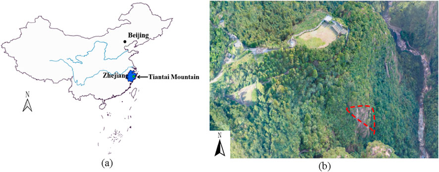
Figure 3. (a) Map of study area (b) General view of slope.

The selected slope showcases a significant variation along the $x$, $y$ and $z$ axes, with measurements under the relative coordinate system indicating a difference of 16.72 m, 12.96 m, and 24.15 m, respectively. Moreover, the maximum slope angle exceeds 80°. For this paper, the TopconGLS-2000 three-dimensional laser scanner was employed to capture the point cloud data, resulting in a total of 384,663 points.

2.8 Methods for error evaluation

At present, in the field of three-dimensional point cloud, the research in the direction of vegetation filtering is still in progress, and manual filtering of vegetation point cloud is still recognized as the most accurate and widely used method. Therefore, new algorithms are proposed to verify the feasibility of the algorithms based on the results of manually filtering the vegetation point cloud. The accuracy of manually filtering the vegetation point cloud is limited by the skill of the operator, and the workload is relatively large, and the time spent is very large, so the algorithm in this paper has a large amount of workload to test.

For the qualitative evaluation of the algorithm’s performance, the results obtained by the proposed method are compared with those derived from manual vegetation point cloud filtering. This comparison assesses the effectiveness of noise removal as well as the preservation of rock mass structural features.

In this study, the effectiveness of the filtering results is assessed quantitatively through the utilization of three error evaluation metrics: class error $I_e$, class error $I{I}_e$ and total error $A_e$. These metrics are calculated using the following formulas (Ding et al., 2019):

$\left\{\begin{array}{l}{I}_e=\frac{OFP}{GP}\times 100\%\\ I{I}_e=\frac{IFP}{OP}\times 100\%\\ A_e=\frac{OFP+IFP}{GP+OP}\times 100\%\end{array}\right.(10)$

In this context, $GP$ represents the count of ground points, $OP$ represents the count of non-ground points, $OFP$ represents the count of points filtered as ground points, and $IFP$ represents the count of points misclassified as ground points. It is evident that class error $I_e$ primarily indicates the occurrence of mistakenly removing ground points. On the other hand, class error $I{I}_e$ highlights the presence of residual vegetation points. Therefore, the combination of class error $I_e$ and class error $I{I}_e$ reflects the algorithm’s applicability. The total error $A_e$ assesses the overall error in the filtering results, thereby indicating the feasibility of the algorithm (Ding et al., 2019).

3 Results

3.1 Experimental results

The value of K is set to 20, the discrete limiting value is set to 0.85, and the discrete value for determining the vegetation seed points using a small window is set to 50% of the overall discrete limiting value. Figures 4a,b showcase the target slope maps obtained through the TopconGLS-2000 three-dimensional laser scanner. To separate the vegetation and rock point clouds, the CloudCompare software was employed manually. The results of this separation are represented by red and blue colors, as depicted in Figures 4c,d.

Figure 4

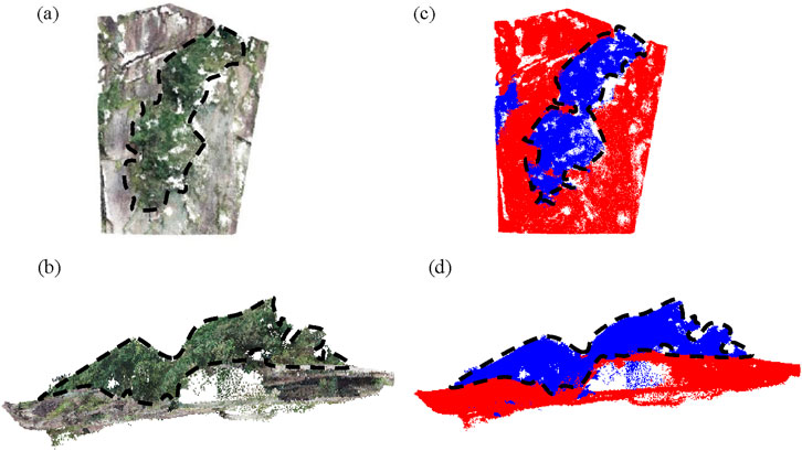
Figure 4. The experimental results prior to filtering. In (a), the rocky and highly steep slopes of Tiantai Mountain are captured from a front view. Similarly, (b) presents the same slopes but from a side view. The manual separation of the red and blue marker maps can be observed in (c,d), providing a front and side view respectively.

Upon applying the proposed filtering algorithm, which integrates K-means clustering, the visualizations of the extracted vegetation and point clouds after vegetation removal are presented in Figures 5a,b. Additionally, Figures 5c,d display the manually marked points.

Figure 5

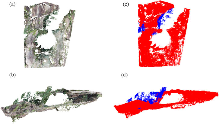
Figure 5. The experimental results obtained after applying the filtering process. The front view of the algorithmically filtered effect map is shown in (a), while (b) presents the side view of the same map. Additionally, (c) exhibits the front view of the algorithmically filtered red and blue marker maps, while (d) showcases the side view of the red and blue marker map after undergoing algorithmic filtering.

By employing Equation 10, the class error $I_e$, class error $I{I}_e$ and total error $A_e$ are calculated. The analysis of the filtering results yields the following values: $I_e=7.72\%$, $I{I}_e=6.86\%$ and $A_e=7.40\%$.

In the above figure, the blue color represents the vegetation point cloud and the red color represents the rock body point cloud, the more blue points are filtered out, the better the result. From Figures 4, 5, the following points can be concluded:

First, the point cloud data model constructed from the original point cloud data Figures 4a,b cannot show the structural surface characteristics, there is vegetation masking, so filtering processing is needed.

Secondly, Figures 4c,d show the data models constructed from the point cloud data obtained by manual filtering. It can be seen that although most of the vegetation noise is removed, the method is limited by the fact that it is difficult to remove the vegetation point cloud in some special terrains due to manual editing.

Finally, the model generated by the proposed algorithm is shown in Figure 5. Most of the vegetation point clouds have been successfully removed, while the rock point cloud data that accurately represent the surface characteristics of the slope are well preserved. Only a small number of scattered vegetation points with minimal impact remain, indicating that the filtering performance is effective and reliable.

3.2 Interpretation results of the rock surface structure

The original point cloud and the K-means algorithm filtered point cloud were substituted into the rock structural surface identification program developed by Wu Faquan’s team (Kong et al., 2020), and the same parameters were selected to decipher the two structural surface classification information, as shown in Figure 6.

Figure 6

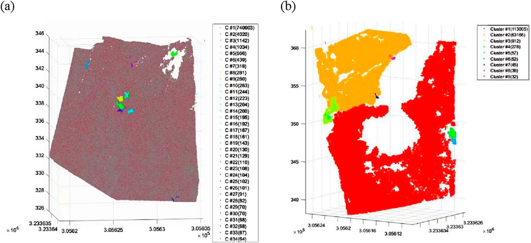
Figure 6. Results of rock structure surface interpretation. (a) Before vegetation filtering; (b) After vegetation filtering (C#1 represents the category index, with the number in parentheses indicating the quantity of point clouds).

After applying the vegetation filtering algorithm, which is based on K-means clustering (with K set to 15), to the point cloud data of the rock mass, the corresponding structural surface information of the rock mass can be obtained. This is illustrated in Figure 6b. The total discrete limit value for this filtering choice is set to 0.84.

The interpretation results show that, in the original unfiltered point cloud, 34 structural surface categories were identified. However, the gray-red point clouds—which account for approximately 97% of the total points—were not effectively classified, indicating significant overlap and noise. After applying the filtering algorithm, the point clouds exhibit markedly improved classification, with more distinct structural surface groupings and a substantial reduction in the number of small, scattered categories. This demonstrates the enhanced clarity and reliability of structural surface identification after vegetation noise removal.

By comparing the decoding results before and after implementing the vegetation filtering algorithm, it becomes evident that the presence of vegetation point cloud information significantly impedes the decoding of the rock mass. However, by utilizing the vegetation filtering algorithm proposed in this paper, there is a notable improvement in deciphering the structural surface information from the rock mass. Therefore, the vegetation filtering algorithm proposed in this paper has excellent application results.

3.3 Qualitative analysis

Firstly, manual filtering, K-means clustering, and PCA processing are performed. Subsequently, the processed data is screened and visualized using the CloudCompare software, thereby enhancing the clarity and intuitiveness of the final outcomes for improved evaluation.

Several crucial points need to be taken into consideration. Firstly, the model incorporates vegetation occlusion and data gaps, which can influence subsequent analysis results. Secondly, although the majority of vegetation noise points are successfully removed from the surface point cloud data, the complexity of the terrain presents challenges for the complete elimination of all vegetation points. As a result, some small protruding vegetation fragments remain in the filtered model. Moreover, vegetation point clouds in close proximity to rock formations may exhibit surface features such as small grass and moss. Therefore, retaining certain near-ground vegetation point cloud data during the filtering process can yield a more realistic representation, enhancing comprehensiveness. Lastly, by utilizing appropriate point cloud processing software to examine the vegetation-filtered point cloud data based on RGB color information and location information, coupled with K-means clustering, effective removal of scattered vegetation points is achieved. It is evident that the majority of scattered vegetation point clouds are successfully eliminated, while retaining the rock point cloud data that better captures the surface characteristics of rocky slopes, along with a portion of the vegetation point cloud data near the rocks.

3.4 Sensitivity analysis and selection of discrete values

3.4.1 Sensitivity analysis of K-value

The effectiveness of this algorithm in filtering and the determination of the number of clusters through the K-value are influenced by the magnitude of the designated discrete value used to distinguish the presence or absence of vegetation. Therefore, as an initial step in the sensitivity analysis, the size of the discrete value was established based on the SRF algorithm, with a selected value of 0.85, as shown in Figure 7a and Table 1. The SRF algorithm is a vegetation filtering method proposed by our team that integrates spatial position and color information of point clouds. The core idea of the method is to identify vegetation seed points based on the spatial differences between rock surfaces and vegetation in the point cloud data. Subsequently, RGB color information is integrated to assist in the removal of vegetation noise and to enhance the overall filtering accuracy. This enabled a sensitivity analysis of the K-value setting. By applying various K-values for filtering and conducting error analysis on the multiple results (please note that the error analysis results are small, hence grid evaluation of the surface feature retention rate was not performed), the outcomes are presented in Table 2. The trend of changes in error analysis results caused by adjustments in threshold settings is illustrated in Figure 7b.

Figure 7

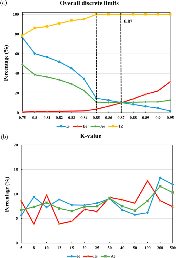
Figure 7. Trend plots of error analysis changes. (a) SRF algorithm; (b) New algorithm based on K-value. (b) demonstrates that with the gradual increase in the number of clusters (K-value), there is no identifiable pattern of change in the errors (Ie, IIe and Ae) in vegetation point cloud filtering. However, it can be observed that a higher or lower K-value does not necessarily result in improved outcomes.

Table 1

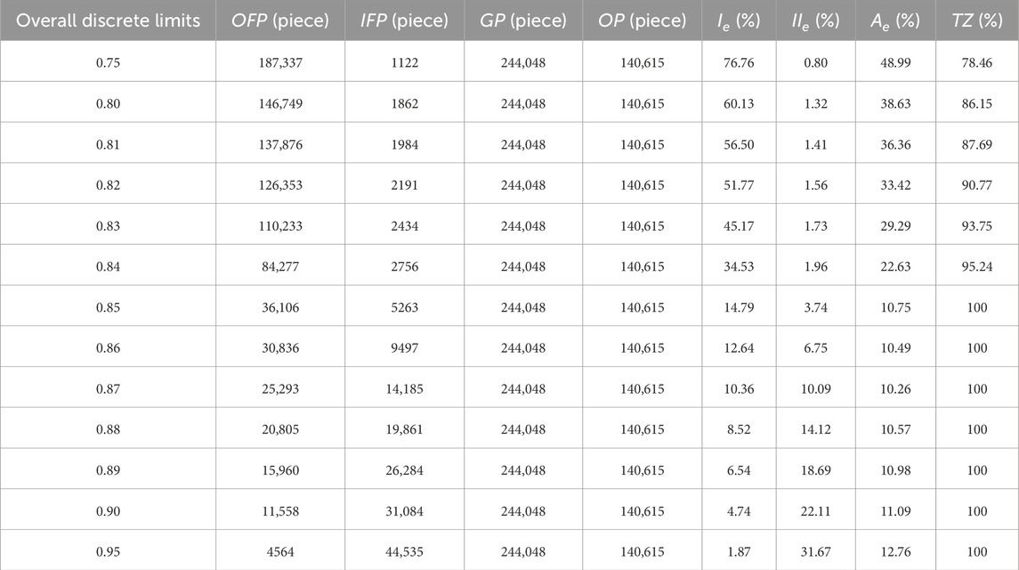
Table 1. SRF algorithm to analyze the results of filtering with different degrees of dispersion.

Table 2

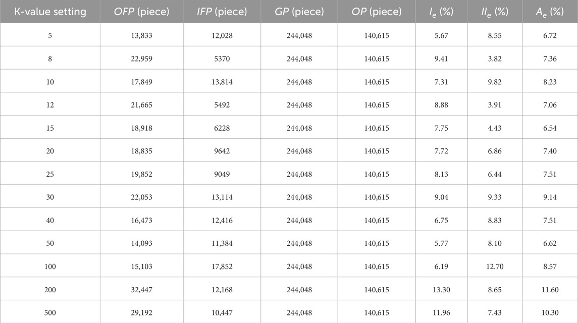
Table 2. Comparison of filtering results for different values of K.

3.4.2 Overall sensitivity analysis of discrete limit values

Based on the aforementioned K-value analysis results, a value of K = 15 is selected to conduct a sensitivity analysis on the set discrete value. Recognizing that different overall discrete threshold settings can affect the filtering outcomes, a range of discrete values is employed for the filtering process. Subsequently, an error analysis is performed on the multiple outcomes obtained. The results of this analysis are presented in Table 3. Additionally, Figure 8 illustrates the trend of the error analysis results as the threshold setting is varied.

Table 3

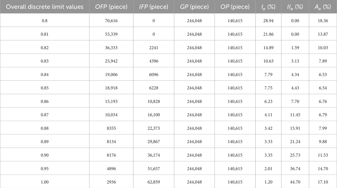
Table 3. A comparison of filtering results for K = 15 with different degrees of dispersion.

Figure 8

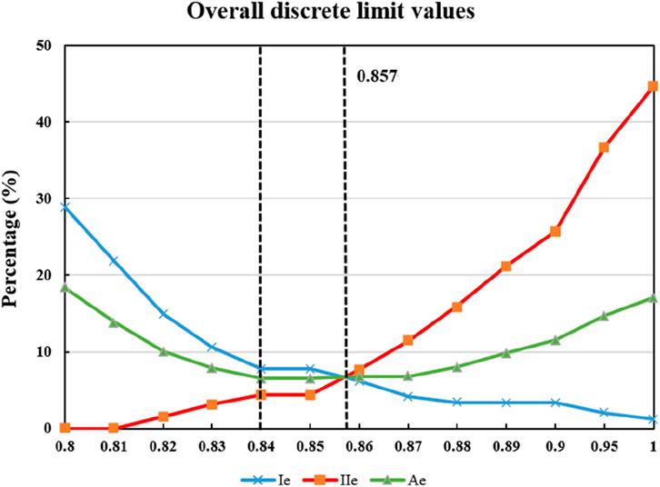
Figure 8. Trend plots of error analysis changes.

Figure 8 illustrates that increasing the overall discrete limit setting gradually reduces the proportion of incorrectly deleted ground points. This can be attributed to the preservation of ground-hugging vegetation point clouds. At the same time, a higher overall discrete limit setting leads to a more pronounced presence of residual vegetation point clouds. Therefore, the overall discrete limit setting plays a crucial role in selecting vegetation points in the algorithm proposed in this paper. Before setting the overall discrete limit value at 0.84, the total error $A_e$ decreases gradually as the overall discrete limit value setting. During this phase, the growth rate of residual vegetation points in the manually selected vegetation points is slower than the rate of reduction in misclassified ground points. However, when the overall discrete limit value setting exceeds 0.84, the overall misclassification ratio starts to increase. Additionally, the ratio of vegetation points in the manually selected vegetation points also increases. Notably, the growth rate of this ratio surpasses the rate of reduction in erroneously deleted ground points.

3.4.3 Selection of overall discrete limit values

To optimize the filtering process and achieve a balance between retaining surface features and minimizing total error ${\mathrm{A}}_{\mathrm{e}}$, the overall discrete limit is set at 0.84. The results of the error analysis show $I_e=7.79\%$, $I{I}_e=4.34\%$ and $A_e=6.53\%$. From the error analysis, it can be observed that the filtering results of the algorithm in this paper, the smaller $I_e$ indicates that the ground points are erroneously deleted more, and the smaller $I{I}_e$ indicates that there are a small number of vegetation points omitted from the deletion. When the overall discrete threshold is set to 0.84, the filtering effect is demonstrated in Figures 9a,b. This process effectively removes a significant amount of vegetation noise points while incidentally eliminating a small number of rock mass point clouds. Despite this, the overall outcome of the filtering is considered satisfactory.

Figure 9

Figure 9. Filtering effect plots for an overall discrete limiting value of 0.84 and K = 15. (a) Front view; (b) Side view.

As shown in Table 3, when the overall discrete limit value is set to 0.81, no residual vegetation point cloud is observed, resulting in error analysis values of $I_e=21.86\%$, $I{I}_e=0\%$ and $A_e=13.87\%$. The error analysis indicates that there are currently no remaining vegetation point cloud data after the filtering process. However, a larger number of ground points have been filtered out, particularly those closely associated with the ground surface. This filtering outcome is visually represented in Figures 10a,b, demonstrating the successful removal of all vegetation-related point clouds while retaining a significant amount of ground point clouds. Nevertheless, it should be noted that this filtering process leads to a loss of information in the smoother rock slope area.

Figure 10

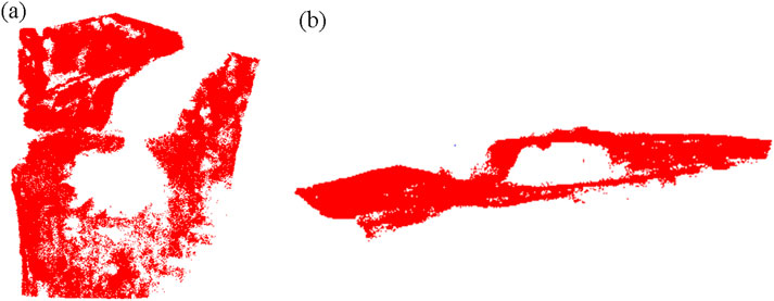
Figure 10. Filtering effect plot for an overall discrete limiting value of 0.81 and K = 15. (a) Front view; (b) Side view.

After applying the K-means clustering algorithm to eliminate vegetation noise points, the original vegetation point cloud still contains scattered points, including a small number of ground points and residual vegetation noise points resulting from laser measurement characteristics. The presence of these residual vegetation noise points can be attributed to several factors, including measurement errors caused by external disturbances (e.g., wind-induced movement of vegetation), the accumulation of dust on vegetation surfaces, and the similarity in color features between residual vegetation and low-lying ground vegetation, which complicates their distinction during filtering. However, it is important to note that these residual vegetation noise points are not completely empty. To further minimize their presence, hierarchical filtering can be employed prior to identifying the structural surface information of the rock mass. This additional step has minimal impact on the identification of the rock mass’s structural surface and the determination of parameters.

As shown in Table 3 and Figure 8, the overall error (Ae) decreases significantly as the discrete threshold increases from 0.80 to 0.84, reaching a minimum of 6.53% at 0.84. This indicates optimal retention of rock surface points while effectively removing vegetation noise. When the threshold exceeds 0.84, Ae starts to rise again, reaching 17.10% at 1.00, primarily due to the preservation of low-lying vegetation points. Therefore, 0.84 represents a critical turning point in balancing the trade-off between vegetation removal and ground point preservation.

Similarly, among all K-values tested (Table 2), K = 15 yields the lowest total error (6.54%) and an acceptable balance between class I and class II errors, confirming its suitability for this dataset. The results show that improper selection of K (e.g., too small like K = 5 or too large like K = 200) can lead to elevated total errors and unstable filtering performance.

Furthermore, a comparative evaluation between our method and manual filtering showed that although manual filtering achieved slightly lower class I error (7.72% vs. 7.75%), it failed to remove complex terrain vegetation effectively, as shown in Figures 4c,d. This demonstrates the advantage of our algorithm in handling intricate slope environments, with improved reproducibility and automation.

4 Discussion

4.1 Algorithm comparison

In this study, the errors in point cloud data accuracy, actual imaging conditions, manual point selection, and other factors are denoted as $I_e$, $I{I}_e$ and $A_e$. The complexity of the mine slope gradient, which varies in reality, is closely examined and analyzed in relation to this study. The comparison and analysis are conducted comprehensively, taking into consideration the findings of other researchers (Ding et al., 2019; Zhang et al., 2013b; Wen et al., 2023). The results are presented in Table 4 and Figure 11. The RGDI algorithm is based on the Red-Green Difference Index proposed by our team. It enhances the contrast between the reflectance values of the red (R) and green (G) spectral bands using a nonlinear stretching method to determine whether a given point belongs to vegetation.

Table 4

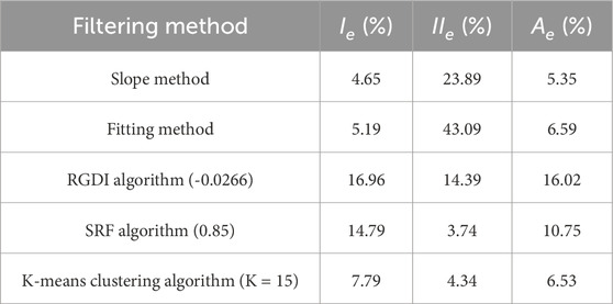
Table 4. Comparison of error analysis of other algorithms.

Figure 11

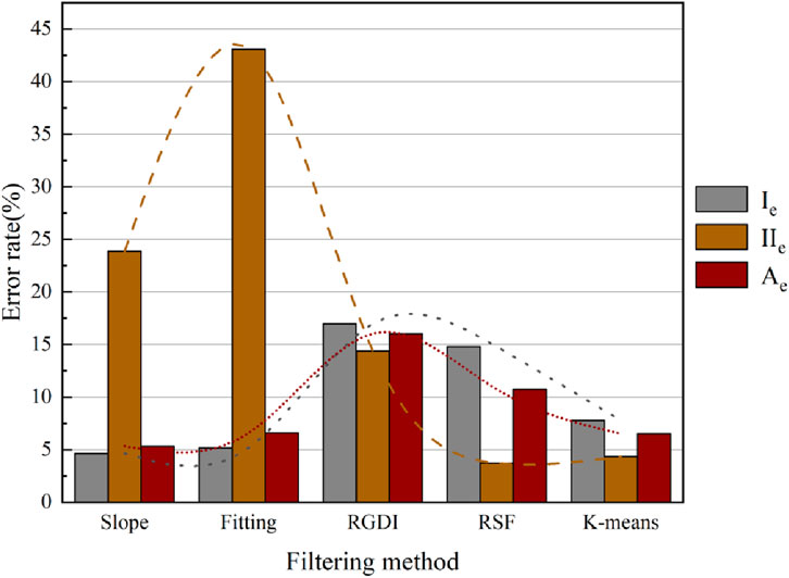
Figure 11. Comparative visualization of error analysis of other algorithms.

The conventional vegetation filtering algorithm often makes incorrect judgments on point clouds, particularly when dealing with mine slopes, resulting in significant deletion of ground points. In this paper, a vegetation filtering algorithm is proposed, which utilizes K-means clustering based on error analysis results. The value of $I_e$ in this algorithm are comparable to those of the Slope and Fitting methods. However, when compared to the RGDI algorithm and the SRF algorithm, the class error $I_e$ is significantly reduced. This reduction can be attributed to the steep rocky slopes investigated in this study, which is reflected in the algorithm’s high retention rate of ground points. Moreover, the algorithm demonstrates a small value of $I{I}_e$ in comparison to the traditional method in the table, indicating its effectiveness in removing noise points caused by green vegetation. Consequently, only a minimal number of residual vegetation point clouds remain. This advantage becomes particularly apparent when compared to the fitting method. Through a comparative analysis of the results displayed in point cloud processing software, it is evident that the proposed algorithm effectively exposes rock features without impeding the subsequent recognition of the structural surface of the rock mass.

4.2 Analysis of advantages and limitations

In contrast to the slope method, the fitting method, and the RGDI threshold filtering algorithm, the algorithm proposed in this paper eliminates the reliance on a fixed threshold. Instead, it dynamically selects thresholds in a swift and flexible manner. Furthermore, the incorporation of a preservation guarantee mechanism significantly improves the retention rate of ground feature points and reduces over-filtering, leading to a remarkable enhancement in filtering effectiveness. When compared to the SRF algorithm, it demonstrates exceptional performance in removing vegetation points while preserving ground points.

The vegetation filtering algorithm presented in this study utilizes K-means clustering and undergoes comprehensive analysis to evaluate its overall performance and sensitivity to discrete values. It showcases outstanding efficacy in processing vegetation point cloud data, with its applicability extending to near-vertical steep slopes. Moreover, it effectively preserves the undulating characteristics of the rock mass’s structural surface, resulting in a superior overall filtering effect.

5 Conclusion

This study focuses on the analysis of three-dimensional laser point cloud data obtained from the high and steep slopes of Tiantai Mountain. An innovative vegetation filtering algorithm utilizing K-means clustering was introduced. The major conclusions are as follows:

1. The proposed algorithm utilizes Principal Component Analysis (PCA) to downscale the spatial location information and Red-Green Difference Index (RGDI) to downscale the RGB color information. This process effectively transforms the initially acquired six-dimensional point cloud data into two dimensions. Subsequently, the data is segmented using K-means clustering.

2. The vegetation filtering algorithm employing K-means clustering successfully isolates a significant number of vegetation noise points while preserving the essential structural attributes of the rock mass. K-means clustering groups point clouds based on their similar spatial and RGB information. Therefore, the choice of K-value does influence the filtering outcome. However, the sensitivity analysis conducted in this study reveals that, currently, no discernible pattern exists in determining its value.

3. In comparison to traditional algorithms, the vegetation filtering algorithm utilizing K-means clustering demonstrates substantial advantages in removing vegetation point clouds on steep slopes. Conventional methods like the slope method and fitting method exhibit suboptimal performance in vegetation removal. On the other hand, the proposed algorithm retains a considerable number of ground points while effectively filtering out a significant portion of the vegetation point clouds. This successful outcome further validates the feasibility of integrating RGB color information to address the vegetation filtering challenge across multiple dimensions on steep slopes.

4. When compared to the other algorithms discussed in this paper, the vegetation filtering algorithm utilizing K-means clustering excels in effectively removing a higher number of vegetation points while preserving a greater number of ground points. This addresses the issue faced by other algorithms that tend to remove a substantial portion of vegetation points along with more ground points.

5. The algorithm presented in this study partially mitigates the issue of over-filtering in vegetation point cloud filtering. Because of the relatively sparse distribution of vegetation, during three-dimensional laser scanning, some ground points hidden by vegetation are captured. The proposed algorithm effectively processes this data, preserving the ground points while removing the vegetation point clouds. Additionally, this algorithm specifically focuses on point cloud data from areas with low to medium vegetation density, which constitutes a significant portion of the dataset. Therefore, the choice of treatment becomes crucial as the source of point cloud data significantly impacts the vegetation filtering approach in this study.

Although the proposed vegetation filtering algorithm based on K-means clustering demonstrates satisfactory performance in removing vegetation noise and preserving essential rock structural features, several limitations remain. First, the effectiveness of the algorithm is partly constrained by the spatial resolution and quality of the point cloud data. High-density vegetation or low-resolution scans may hinder accurate noise identification. Second, the selection of algorithmic parameters—such as the K value in clustering, the threshold for deviation from the fitted plane, and the grid size for seed point generation—introduces a degree of subjectivity and may vary depending on terrain characteristics. Third, while qualitative and quantitative assessments were performed in this study, validation still relies on comparison with manual filtering, which itself may contain inherent uncertainties.

Future research should focus on enhancing the automation and adaptability of the algorithm, for instance by introducing adaptive parameter tuning or integrating machine learning-based vegetation classifiers. In addition, testing the method on a wider range of slope types and geological settings will help generalize its applicability. Incorporating multispectral or hyperspectral data could also further improve vegetation-rock discrimination, especially in densely vegetated or shaded regions.

Data availability statement

The datasets presented in this article are not readily available because the dataset is not publicly available due to confidentiality agreements or fieldwork privacy concerns. Requests to access the datasets should be directed to MjY1NDA3Nzk0N0BxcS5jb20=.

Author contributions

SG: Writing – review and editing, Conceptualization. MY: Data curation, Validation, Writing – review and editing. JL: Formal analysis, Writing – review and editing. XL: Writing – original draft. FW: Conceptualization, Writing – review and editing. ZS: Investigation, Methodology, Writing – review and editing. HZ: Investigation, Writing – original draft.

Funding

The author(s) declare that financial support was received for the research and/or publication of this article. This work was supported by the Central Government’s Guidance Fund Projects for Local Science and Technology Development (Grant No. 2024ZY01041); the Zhejiang Provincial Natural Science Foundation of China (Grant No. LHQ20D020001); and the Major Project of the National Natural Science Foundation of China (Grant No. 41831290).

Acknowledgments

The authors would like to thank the reviewers for their insightful comments and constructive suggestions, which greatly improved the quality of this article.

Conflict of interest

The authors declare that the research was conducted in the absence of any commercial or financial relationships that could be construed as a potential conflict of interest.

Generative AI statement

The author(s) declare that no Generative AI was used in the creation of this manuscript.

Any alternative text (alt text) provided alongside figures in this article has been generated by Frontiers with the support of artificial intelligence and reasonable efforts have been made to ensure accuracy, including review by the authors wherever possible. If you identify any issues, please contact us.

Publisher’s note

All claims expressed in this article are solely those of the authors and do not necessarily represent those of their affiliated organizations, or those of the publisher, the editors and the reviewers. Any product that may be evaluated in this article, or claim that may be made by its manufacturer, is not guaranteed or endorsed by the publisher.

References

Błaszczak-Bąk, W., Janowski, A., Kamiński, W., and Rapiński, J. (2011). Optimization algorithm and filtration using the adaptive TIN model at the stage of initial processing of the ALS point cloud. Can. J. Remote Sens. 37 (6), 583–589. doi:10.5589/m12-001

CrossRef Full Text | Google Scholar

Chen, J., Zhao, D., Zheng, Z., Xu, C., Pang, Y., and Zeng, Y. (2024). A clustering-based automatic registration of UAV and terrestrial LiDAR forest point clouds. Comput. Electron. Agric. 217, 108648. doi:10.1016/j.compag.2024.108648

CrossRef Full Text | Google Scholar

Chong, B. (2021). K-means clustering algorithm: a brief review. Acad. J. Comput. and Inf. Sci. 4 (5), 37–40. doi:10.25236/AJCIS.2021.040506

CrossRef Full Text | Google Scholar

Ding, S., Liu, R., Cai, Y., and Wang, P. (2019). A point cloud adaptive slope filtering method considering terrain. Remote Sens. Inf. 34, 108–113. doi:10.3969/j.issn.1000-3177.2019.04.017

CrossRef Full Text | Google Scholar

Giuseppe, O. (2023). A filtering monotonization approach for DG discretizations of hyperbolic problems. Comput. Math. Appl. 129, 113–125. doi:10.1016/j.camwa.2022.11.017

CrossRef Full Text | Google Scholar

Havens, T. C., Bezdek, J. C., Leckie, C., Hall, L. O., and Palaniswami, M. (2012). Fuzzy c-means algorithms for very large data. IEEE Trans. Fuzzy Syst. 20, 1130–1146. doi:10.1109/tfuzz.2012.2201485

CrossRef Full Text | Google Scholar

Jia, S., Jin, A., and Zhao, Y. (2018). Application of UAV oblique photogrammetry in the field of geology survey at the high and steep slope. Rock Soil Mech. 39, 1130–1136. doi:10.16285/j.rsm.2017.1474

CrossRef Full Text | Google Scholar

Jothiaruna, N., Sundar, A. J. K., and Ahmed, I. M. (2020). A disease spot segmentation method using comprehensive color feature with multi-resolution channel and region growing. Multimedia Tools Appl. 80 (3), 1–9. doi:10.1007/s11042-020-09882-7

CrossRef Full Text | Google Scholar

Kong, D., and Wu, F.CharalamposSaroglou (2020). Automatic identification and characterization of discontinuities in rock masses from 3D point clouds. Eng. Geol. 265, 105442. doi:10.1016/j.enggeo.2019.105442

CrossRef Full Text | Google Scholar

Li, T., Sun, S., Corchado, J. M., and Sattar, T. P. (2016). Numerical fitting-based likelihood calculation to speed up the particle filter. Int. J. Adapt. Control Signal Process. 30 (11), 1583–1602. doi:10.1002/acs.2656

CrossRef Full Text | Google Scholar

Lin, H., and Du, Z. (2013). Some problems in comprehensive evaluation in the principal component analysis. Stat. Res. 30, 25–31. doi:10.19343/j.cnki.11-1302/c.2013.08.004

CrossRef Full Text | Google Scholar

Meng, X., Currit, N., and Zhao, K. (2010). Ground filtering algorithms for airborne LiDAR data: a review of critical issues. Remote Sens. 2 (3), 833–860. doi:10.3390/rs2030833

CrossRef Full Text | Google Scholar

Mikita, T., Klimánek, M., and Cibulka, M. (2013). Evaluation of airborne laser scanning data for tree parameters and terrain modelling in forest environment. Acta Univ. Agric. Silvic. Mendelianae Brunensis 61 (5), 1339–1347. doi:10.11118/actaun201361051339

CrossRef Full Text | Google Scholar

Mongus, D., and Žalik, B. (2012). Parameter-free ground filtering of LiDAR data for automatic DTM generation. ISPRS J. Photogrammetry Remote Sens. 67, 1–12. doi:10.1016/j.isprsjprs.2011.10.002

CrossRef Full Text | Google Scholar

Mu, X., Zhu, Y., Dou, K., Shi, Y., and Huang, M. (2024). Logging response prediction of high-lithium coal seam based on K-means clustering algorithm. Front. Earth Sci. 12, 1443458. doi:10.3389/feart.2024.1443458

CrossRef Full Text | Google Scholar

Nie, S., Wang, C., Dong, P., Xi, X., Luo, S., and Qin, H. (2017). A revised progressive TIN densification for filtering airborne LiDAR data. Measurement 104, 70–77. doi:10.1016/j.measurement.2017.03.007

CrossRef Full Text | Google Scholar

Pugazhenthi, A., and Kumar, L. S. (2020). Automatic cloud segmentation from INSAT-3D satellite image via IKM and IFCM clustering. IET Image Process. 14(7), 1273–1280. doi:10.1049/iet-ipr.2018.5271

CrossRef Full Text | Google Scholar

Shi, Z., Fan, J., Du, Y., Zhou, Y., and Zhang, Y. (2024). LULC-SegNet: enhancing land use and land cover semantic segmentation with denoising diffusion feature fusion. Remote Sens. 16 (23), 4573. doi:10.3390/rs16234573

CrossRef Full Text | Google Scholar

Sihong, T., Huapeng, Z., and David, Z. C. (2021). An adaptive sampling strategy based on region growing for near-field-based imaging of radiation sources. IEEE Access 9, 9550–9556. doi:10.1109/access.2021.3051071

CrossRef Full Text | Google Scholar

Simoniello, T., Coluzzi, R., Guariglia, A., Imbrenda, V., Lanfredi, M., and Samela, C. (2022). Automatic filtering and classification of low-density airborne laser scanner clouds in shrubland environments. Remote Sens. 14 (20), 5127. doi:10.3390/rs14205127

CrossRef Full Text | Google Scholar

Sud, K., Erdogmus, P., and Kadry, S. (2020). Introduction to data science and machine learning.

Google Scholar

Susaki, J. (2012). Adaptive slope filtering of airborne LiDAR data in urban areas for digital terrain model (DTM) generation. Remote Sens. 4 (6), 1804–1819. doi:10.3390/rs4061804

CrossRef Full Text | Google Scholar

Tang, L., Wang, S., Zhou, M., Ding, Y., Wang, C., Wang, S., et al. (2023). Research on recognition algorithm for gesture page turning based on wireless sensing. Intelligent Converged Netw. 4, 15–27. doi:10.23919/icn.2023.0002

CrossRef Full Text | Google Scholar

Tingting, Y., Yinuo, Z., Yan, Z., Yang, W., Dong, J., Liu, X., et al. (2023). Impacts of climate change and human activities on vegetation coverage variation in mountainous and hilly areas in Central South of Shandong Province based on tree-ring. Front. Plant Sci. 14, 1158221. doi:10.3389/fpls.2023.1158221

PubMed Abstract | CrossRef Full Text | Google Scholar

Turkes, C. M. (2017). Cluster analysis of total assets provided by banks from four continents. Acad. J. Econ. Stud. 3 (4), 24–28.

Google Scholar

Wan, P., Zhang, W., Skidmore, A. K., Qi, J., Jin, X., Yan, G., et al. (2018). A simple terrain relief index for tuning slope-related parameters of LiDAR ground filtering algorithms. ISPRS J. Photogrammetry Remote Sens. 143, 181–190. doi:10.1016/j.isprsjprs.2018.03.020

CrossRef Full Text | Google Scholar

Wen, H., Hu, J., Xiong, F., Zhang, C., Song, C., and Zhou, X. (2023). A random forest model for seismic-damage buildings identification based on UAV images coupled with RFE and object-oriented methods. Nat. Hazards 119 (3), 1751–1769. doi:10.1007/s11069-023-06186-5

CrossRef Full Text | Google Scholar

Xing, S., Li, P., Xu, Q., Wang, D., and Li, P. (2017). Surface fitting filtering of LiDAR point cloud with waveform information. ISPRS Annals of the Photogrammetry. Remote Sens. Spatial Inf. Sci. 4, 179–184. doi:10.5194/isprs-annals-IV-2-W4-179-2017

CrossRef Full Text | Google Scholar

Xu, Q. Y. (2014). Massive data analysis based MapReduce structure on Hadoop system. Adv. Mater. Res. 981, 262–266. doi:10.4028/www.scientific.net/amr.981.262

CrossRef Full Text | Google Scholar

Yan, Y., Chen, Z., Sun, Y., Li, Z., and Yao, C. (2021). LiDAR point cloud ground filtering algorithm in dense and low vegetation area. Bull. Surv. Mapp. (07), 1–5. doi:10.13474/j.cnki.11-2246.2021.0199

CrossRef Full Text | Google Scholar

Yang, L., and Zhai, R. (2019). Segmentation of plant organs point clouds through super voxel-based region growing methodology. Comput. Eng. Appl. 55, 197–203. doi:10.3778/j.issn.1002-8331.1805-0221

CrossRef Full Text | Google Scholar

Zhang, J., and Lin, X. (2013a). Filtering airborne LiDAR data by embedding smoothness-constrained segmentation in progressive TIN densification. ISPRS J. Photogrammetry Remote Sens. 81, 44–59. doi:10.1016/j.isprsjprs.2013.04.001

CrossRef Full Text | Google Scholar

Zhang, W., Chen, J., Wang, Q., Ma, D., Niu, C., and Zhang, W. (2013b). Investigation of RQD variation with scanline length and optimal threshold based on three-dimensional fracture network modeling. Sci. China Technological Sci. 56, 739–748. doi:10.1007/s11431-013-5132-6

CrossRef Full Text | Google Scholar

Zhao, C., Gong, W., Juang, C. H., Tang, H., Hu, X., and Wang, L. (2023). Optimization of site exploration program based on coupled characterization of stratigraphic and geo-properties uncertainties. Eng. Geol. 317, 107081. doi:10.1016/j.enggeo.2023.107081

CrossRef Full Text | Google Scholar

Zheng, H., Shi, Z., Yu, S., Fan, X., Hanley, K. J., and Feng, S. (2021). Erosion mechanisms of debris flow on the sediment bed. Water Resour. Res. 57 (12), e2021WR030707. doi:10.1029/2021wr030707

CrossRef Full Text | Google Scholar

Zheng, H., Hu, X., Shi, Z., Shen, D., and De Haas, T. (2024). Deciphering controls of pore-pressure evolution on sediment bed erosion by debris flows. Geophys. Res. Lett. 51 (5), e2024GL108583. doi:10.1029/2024gl108583

CrossRef Full Text | Google Scholar

Zhou, J., Chen, J., and Li, H. (2024). An optimized fuzzy K-means clustering method for automated rock discontinuities extraction from point clouds. Int. J. Rock Mech. Min. Sci. 173, 105627. doi:10.1016/j.ijrmms.2023.105627

CrossRef Full Text | Google Scholar