 Christelle Hély
 Herman H. Shugart
 Robert J. Swap4
 Cédric Gaucherel
- 1Institut des Sciences de l’Evolution de Montpellier (ISEM), Montpellier University, CNRS, EPHE, IRD, Montpellier, France
- 2EPHE, PSL University, Paris, France
- 3Department of Environmental Sciences, University of Virginia, Charlottesville, VA, United States
- 4Sciences and Exploration Directorate, Goddard Space Flight Center, NASA, Greenbelt, MD, United States
- 5AMAP – INRA, CIRAD, CNRS, IRD, Montpellier University, Montpellier, France
There are many ways to study ecosystem dynamics, all having several issues. Main limitations of differential equation systems are the necessarily small number of interactions between few variables used, and parameter values to be set before the system dynamics can be studied. Main drawbacks of large-scale snapshot observation datasets to build a stability landscape are assuming that the most represented conditions are the most stable states, and using the computed landscape to directly study the system’s dynamics. To remedy these aforementioned shortcomings and study complex systems based on the processes that characterize them without having to limit the number of variables, neither set parameter values, nor to use observations serving both model buildup and system’s dynamics analysis, we propose a geometric model as an additional and novel aid to study ecosystem dynamics. The Drape is a generic multi-dimensional analysis, derived from process-based model datasets that include disturbances. We illustrate the methodology to apply our concept on a continental-scale system and by using a mechanistic vegetation model to obtain values of state variables. The model integrates long-term dynamics in ecosystem components beyond the theoretical stability and potential landscape representations currently published. Our approach also differs from others that use resolution of differential equation systems. We used Africa as example, representing it as a grid of 9395 pixels. We simulated each pixel to build the ecosystem domain and then to transform it into the Drape – the mean response surface. Then, we applied a textural analysis to this surface to discriminate stable states (flat regions) from unstable states (gradient or crest regions), which likely represent tipping points. Projecting observed data onto the Drape surface allows testing ecological hypotheses, such as illustrated here with the savanna-forest alternative stable states, that are still today debated topics, mainly due to methods and data used. The Drape provides new insights on all ecosystem types and states, identifying likely tipping points (represented as narrow ridges versus stable states across flat regions), and allowing projection and analysis of multiple ecosystem types whose state variables are based on the same three variables.
1 Introduction
Prediction of ecosystem change under novel conditions is a central issue for ecologists, especially with the apprehension that environmental changes are on multiple scales. A growing number of studies have investigated ecosystem dynamics and their role in planetary function as bases for projecting the Earth’s future (e.g. Brook et al., 2013; Hughes et al., 2013a). From theoretical considerations of system dynamics, one may expect sharp changes can be a part of the dynamic ecosystem repertoire (Scheffer et al., 2001; Briske et al., 2010). Such changes have been analyzed for a diverse array of systems ranging from the Earth climate system (e.g. Lenton et al., 2008; Kriegler et al., 2009; Gaucherel and Moron, 2015), to the international financial system, and to terrestrial and aquatic ecosystems (e.g. Davis and Shaw, 2001; Chapin et al., 2004; Folke et al., 2004; Van Nes and Scheffer, 2007; Favier et al., 2012; Hughes et al., 2013a; Conversi et al., 2015; Martin et al., 2020). Such non-linear responses can profoundly affect the dynamics and management of natural systems (Scheffer et al., 2001).
For almost a century (Lotka, 1925; Volterra, 1926) with increased intensity since the 1970s (Holling, 1973; Noy-Meir, 1975; May, 1977; Walker et al., 1981), ecologists have developed models of ecosystem dynamics. Initially, these were for simplified systems such as predator–prey or competition interactions with the numbers of different populations defined as state variables. If needed, other components representing the environment are also defined as equation parameters.
Such models are often based on systems of ordinary differential equations (ODE). Qualitative or more complex models were first more conceptual, such as state-and-transition models (e.g. Ellis and Swift, 1988; Archer, 1989; Westoby et al., 1989). The use of ODE systems makes more tractable (analytically or numerically) the search for stationary points of the system (i.e. equilibria or periodic orbits) in the so-called phase portrait of the state variables, at least for ecosystem representations of small dimensions. One can characterize the equilibrium stability, which depends on the real part of the eigenvalues of the Jacobian matrix (for hyperbolic equilibria). By analyzing the nullclines, manifolds that go through the fixed points on the phase portrait, the behavior of system-dynamic solutions on the state space can be discerned. Ideally, the local stability of the dynamics is guaranteed by a potential function (in blue on Figure 1A), whose time derivative along the solutions of the system is negative, at least locally. If it is not strictly decreasing everywhere, then multiple steady states or periodic orbits occur, as do bifurcation points (i.e. tipping points) and hysteresis (e.g. May, 1977; Sternberg, 2001).
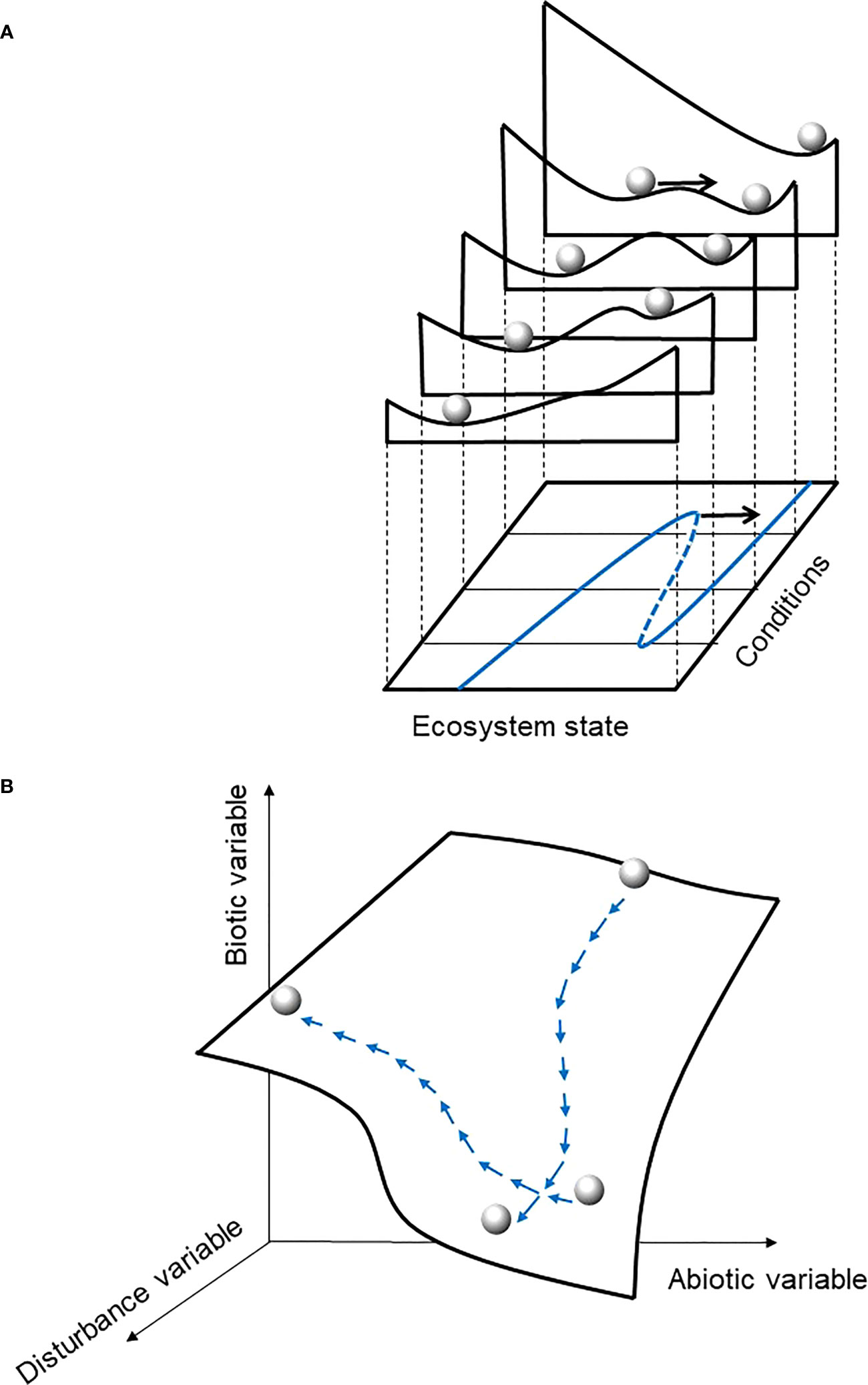
Figure 1 Conceptual representations of ecosystem dynamics (A) from ordinary differential equation system (adapted from Scheffer et al., 2001) or statistical method based on derivative of probability density function (Hirota et al., 2011; Scheffer et al., 2012) and (B) from the present study Drape concept. In both panels, the ball represents the system state at a given time. In (A) the black arrow represents a perturbation (disturbance, stochasticity, noise), considered as an external factor, that pushes the system to another place on the stability landscape (a narrow environmental range slice), on the potential landscape (all slices so the full environmental range), and likely to another equilibrium state (valley) if the ball crosses a ridge; the blue line represents the equilibria curve for this system. In panel (B), the perturbation is stochastic and intrinsic to the vegetation model that created the data, and natural disturbance is embedded in the vegetation model and the system definition. The system may move on the Drape when state variable values change (i.e. at least in terms of climate known as an ongoing changing compartment of the system), which is ineluctable through time, even in terms of small changes. Conversely to the potential landscape in (A) the Drape topography in (B) is not related to the value distribution of each state variable dataset. See Figure 2 for further explanation.
Subsequent studies have advanced in several different directions including: i) determination of leading indicators (also called early warning signal, e.g. Van Nes and Scheffer, 2007; Dakos et al., 2008, 2010; Livina et al., 2010), used to assess the proximity of a system to a tipping point; ii) the role of noise or variability in the system dynamics and intermediate stability creation (e.g. D’Odorico et al., 2005; Dakos et al., 2012); iii) linkage to spatial dynamics and patterns (e.g. van de Koppel et al., 2002; van de Koppel and Rietkerk, 2004; Bel et al., 2012; Kéfi et al., 2014; Ratajczak et al., 2017b); iv) analysis of the response to perturbations of finite magnitude and duration – instead of theoretical developments based on linear stability to infinitesimal perturbations (Ratajczak et al., 2017a) or even the response to continuous stochastic perturbations (Nolting and Abbott, 2016); v) use of space-for-time substitutions and related probability density functions built exclusively from observations in order to infer the potential shape as well as the presence of multiple stable states and tipping points (e.g. Hirota et al., 2011; Staver et al., 2011a; Favier et al., 2012; Scheffer et al., 2012).
Tipping points usually occur in response to a gradual change in a system process (internal and acting on parameter values) or in a system driver (external factor acting on state variables). Under an abrupt change in system state after crossing a tipping point, the system behavior is radically different from that previously observed. Despite intrinsic differences, many dynamic systems display similar early warnings signals prior to the occurrence of a tipping point. These include slowing rates (e.g. Wissel, 1984; Van Nes and Scheffer, 2007), temporal and spatial autocorrelations among system variables (Dakos et al., 2010; Boulton et al., 2013; Kéfi et al., 2014), and fluctuations of the variance increasing up to “flickering” (Wang et al., 2012; Dakos et al., 2013). Active debates regarding tipping points, their nature (Gaucherel et al., 2020), and detection mostly have origins from the catastrophe theory (Thom, 1972).
For global change, terrestrial ecosystem responses are conditioned by many interdependent processes (e.g. Brook et al., 2013; Hughes et al., 2013a). Catastrophic dynamics such as tipping point-events seem relatively rare among ecosystem behaviors. Concepts intending to capture ecosystem dynamics as a whole should also account for the wide range of smooth (gradual) and/or relatively stable behaviors often observed in nature (Dutta et al., 2018). Inclusion of the internal processes responsible for the system dynamics, even in a synthetic and simplified way, provides a better understanding of past and current dynamics by making explicit explanations of the processes. Such inclusion can also improve representation and visualization of concepts such as stable, transient, or alternative states, and system trajectories and system tipping points, if they exist (e.g. Boettiger et al., 2013; Dutta et al., 2018). Nolting and Abbott (2016) showed that to properly detect and study alternative stable states, linear stability analysis, as in traditional deterministic ODE models, is not appropriate to study the potential, thereby necessitating the inclusion of stochasticity.
While using snapshot measurements from extensive datasets is relevant to describe current patterns (e.g. Hirota et al., 2011; Staver et al., 2011a; Scheffer et al., 2012), a number of studies of different ecosystem types and different time scales showed significant discrepancies when testing the space-for-time substitution approach (e.g. Adler and Levine, 2007; Blois et al., 2013). Different observed localities may not have undergone the same historical changes (e.g. disturbance types and regimes), and so, their use in space-for-time analyses may be inappropriate. Interpretations of the underlying ecosystem dynamics (including definitions of equilibria and alternative stable states) should be performed with caution when using the space-for-time substitution approach. This justification is particularly true if these interpretations are not linked to nor validated by a deterministic model, a point wisely suggested by several authors (e.g. Boettiger et al., 2013; Dutta et al., 2018). Fortunately, an increasing number of studies both rely on ecosystem models built with deterministic or stochastic skeletons and then use statistical approaches to compute and test early warning signals, existence of tipping points, and multiple stable states (e.g. Staver et al., 2011b). To analyze the dynamics of a large-scale system, where multiple system states can appear in the studied region as a result of different underlying processes at play, it may be difficult or intractable to rely on a complicated differential equation system. This likely explains why several studies have chosen to statistically analyze observations to differently apprehend the potential and its associated stabilities on the so-called landscape stability (Hirota et al., 2011; Scheffer et al., 2012). This type of applications exhibits several limitations. For instance, the attribution of stable states to the most frequently represented states (and reversely for unstable states) has been criticized (Ratajczak and Nippert, 2012).
From Tansley’s (1935) original ecosystem definition, ecosystems are composed of biotic and abiotic components. It would then be logical to expect an ecosystem to include complexities and interactions beyond merely the populations of organisms it contains (e.g. Gignoux et al., 2011; Gaucherel, 2014). While there are a number of current models that account for abiotic processes, most if not all of them significantly simplify these processes: i) abiotic considerations are reduced to a single limiting-nutrient variable or a synthetic single parameter “resource”; ii) natural disturbances are rarely included in the system definition or considered as parameters only (e.g. D’Odorico et al., 2005; Van Nes et al., 2014; Touboul et al., 2018); iii) dynamics depends on the systems perturbation, considered as either a change in the abiotic resource or in the biotic variable resulting from exogenous factor or from intrinsic stochasticity (e.g. Beisner et al., 2003; Bel et al., 2012).
Many authors have used the so-called ball-in-cup analogy (Figure 1A) to illustrate the system (i.e. the ball) and its dynamics, represented as the movement of the ball along the cup-shaped landscape (e.g. Scheffer et al., 2001; Beisner et al., 2003; Nolting and Abbott, 2016). Regarding ecological systems, Beisner et al. (2003) showed that the concept of alternative stable states was initially apprehended by two different schools (the “community perspective” and the “ecosystem perspective”, respectively), which can be integrated into a common conceptual framework. From the community perspective, the environment, defined by the state variables and the associated potential and landscape stability, is fixed. Conversely, from the ecosystem perspective, the topology of the environment is not fixed because it depends on the parameter values that may change and, in turn, impact state variables. There is therefore an interest in developing tools that allow integrative understanding and visualization of system dynamics. Moreover, for an applied perspective of managing ecosystems, Beisner et al. (2003) also suggest that we should seek to define the boundaries of desirable stable states, and understand the processes that bring resilience nearby these desirable states.
The present work aims to propose a new concept of understanding ecosystem dynamics, the Drape, designed to circumvent some of the aforementioned limitations. It is designed to explore new and likely more informative avenues to understanding ecosystem dynamics. We propose a novel approach, one that is not based on differential equations, to elucidate ecosystem dynamics, across vast spatial scales able to encompass several ecosystems and biomes. Rather than employing more traditional approaches that rely heavily upon differential equations, we use a mechanistic model (mainly deterministic but with some stochasticity) to extract the main state variables (abiotic, biotic, and disturbance, respectively), from which we build two multidimensional representations of the system (the 3D-domain and the 2D-Drape, respectively). We then perform a textural analysis of the Drape, which characterizes its “topography” (variations) in terms of number of stable, unstable and transient states, and their locations on the Drape. Below, we present the Drape theoretical framework, and then illustrate it with African ecosystems and biomes to test several ecological hypotheses before discussing its benefits and limitations.
2 Materials and methods
2.1 Theoretical framework
2.1.1 General characteristics
Following Tansley’s (1935) original definition of the ecosystem as a systems of biotic and abiotic parts and explicitly including disturbances (see Drukenbrod et al. (2019) for a recent review), a minimal ecosystem representation must be multi-dimensional (Figure 1B), with at least three dimensions based on the three most important abiotic, biotic components and disturbance factors (variables), respectively (Gignoux et al., 2011; Gaucherel, 2014). These are the properties of the “conceptual space” used here to capture ecosystem dynamics.
For terrestrial ecosystems, climate conditions are often considered as the main abiotic factor at the continental scale and the vegetation as the main biotic factor. Fire, grazing, or pest outbreak are example of a dominant disturbance (e.g. Pickett and White, 1985; Johnson, 1992; Scholes and Walker, 1993; Sankaran et al., 2005; Staver et al., 2011b). These three minimal factors may provide the synthetic state variables of the system (Figure 1B). For example: 1) annual rainfall, rainfall seasonality or growth season temperature could serve as proxies for the abiotic factor of climate; 2) biomass, leaf area index or tree cover could serve as proxies for the biotic factor; 3) and frequency or return time interval for the main disturbance factor. This representation considers disturbance to be an endogenous variable, unlike the consideration of disturbance as an exogenous factor if considered as the system perturbation, or simply as a limiting parameter in many studies (e.g. Carpenter et al., 2001; Scheffer et al., 2001; Touboul et al., 2018).
All three variables define the ecosystem. This second property is compulsory in this conceptual space: state variables are fully “symmetric” (i.e. interchangeable). The ecosystem is not (purely) biotic, neither is it abiotic. Consequently, an (eco)system could be represented by any of the six permutations of a 3D-space, considering how each state variable may act on the other two through various feedbacks (Scheffer et al., 2005, 2012; Hirota et al., 2011). While vegetation response is usually analyzed as a function of the climate and of the main disturbance, it may be relevant for example to analyze the ecosystem disturbance as a function of the two other factors, as performed in several paleoecological studies (e.g. Hély et al., 2010, Hély et al., 2020; Ali et al., 2012; Aleman et al., 2013).
To illustrate this new approach, we selected Africa as example because this continent encompasses a wide range of environmental conditions and ecosystem types that are all driven by rainfall as the main abiotic variable and most of them as well by fire as the main natural disturbance. We first focused on testing ecological hypotheses related to the forest and savanna states and transitions (see section 2.1) as this is still an ongoing debated topic due to methods used (e.g., Hirota et al., 2011; Ratajczak and Nippert, 2012; Hanan et al., 2014, Hanan et al., 2015; Staver and Hansen, 2015; Aleman et al., 2020). Therefore, the 3D-space for the African terrestrial tropics has been defined using annual rainfall as the climate axis, aboveground biomass as the vegetation axis, and fire frequency (number of fires per year over a fixed interval, e.g. 500 years) as the disturbance axis (Figure 2A). Fire is indeed a major disturbance in these ecosystems (e.g. Scholes and Walker, 1993; Bond et al., 2005; Staver et al., 2011a). Tropical fires currently shifting from natural to human-induced fires could be included to produce a four-dimensional space with a fourth, human-related state variable (Cincotta et al., 2000), if so desired. Numerous studies indicate for instance that tropical forests and savannas are two dominant states that can coexist under the same environmental conditions (e.g. Sankaran et al., 2005; Staver et al., 2011b; Favier et al., 2012). Alternations from one state to the other presumably reflect changes within the environment. Therefore, a third rule in building our example conceptual space is to consider a spatial extent large enough to encompass broad changes within biomes (different savanna ecosystems based on tree cover changes or grass composition changes (e.g. Ringrose et al., 1998; Scholes et al., 2002)), and between biomes (i.e. regime shifts and/or alternation between savannas and forests). Therefore, thanks to this new approach, we were also able to characterize all other ecosystems (from desert to tropical rainforests) and their states on the Drape based on their location and their neighborhood heterogeneity.
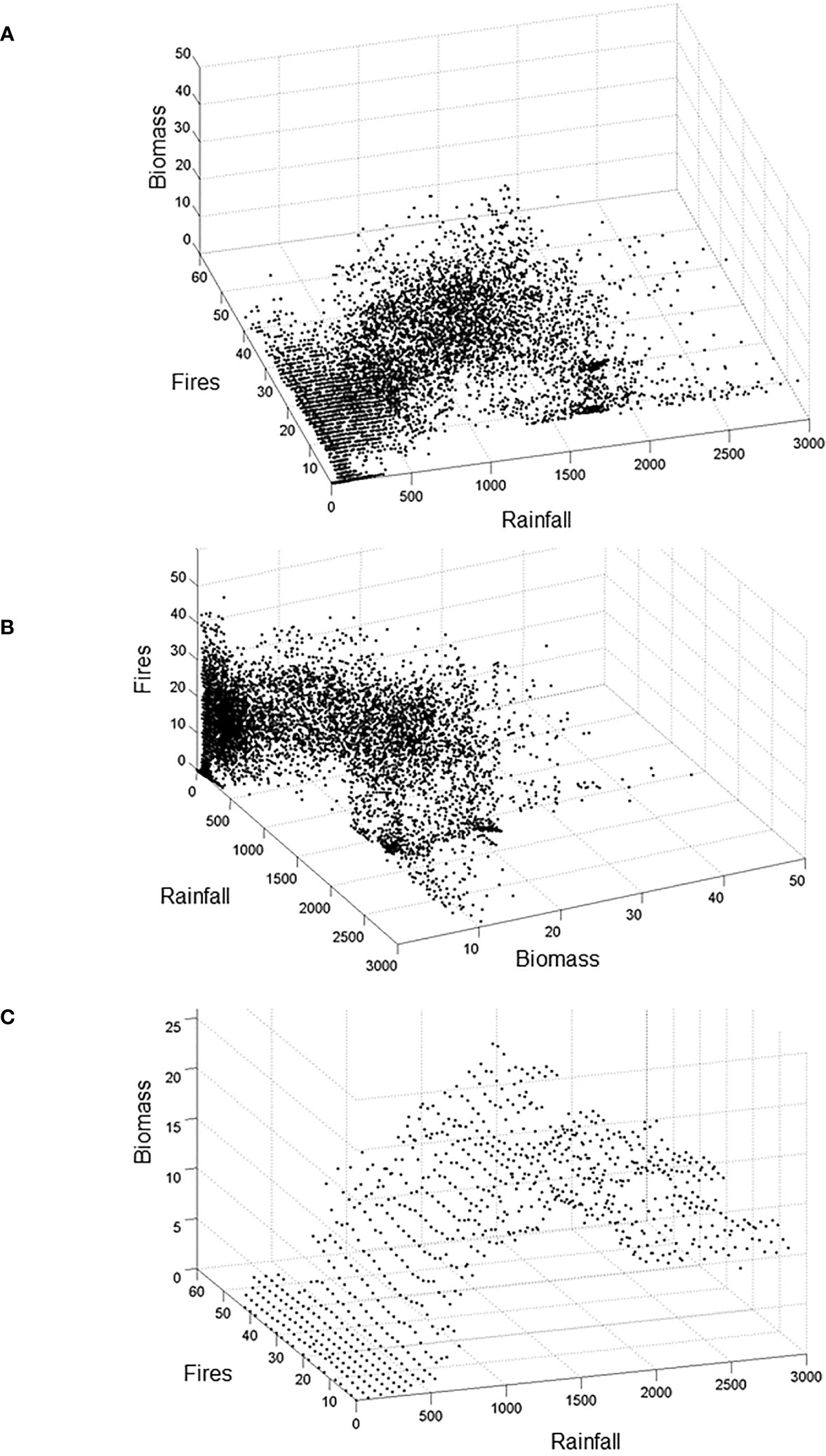
Figure 2 Representations of the tropical domain (cloud of points) within the ecosystem 3D-space. This space is defined by annual Rainfall (in mm.year−1), vegetation carbon Biomass (in kg C.m−2), and Fire (i.e. number of significant fires over 500 years, see Supplementary Figure 1B for computation details), each one representing the most important abiotic, biotic, and disturbance state variables of the system, respectively. In this example, each cloud point represents a continental geographical location in Africa for which the LPJ-GUESS Model (Smith et al., 2001; Sitch et al., 2008) has been previously run (Hély et al., 2006; Gaucherel et al., 2008) using modern climate from the CRU time-series datasets (New et al., 2002). Each point represents the equilibrium state reached by the DGVM at that location, such equilibrium being defined by values of the state variables (see Supplementary Figure S1). (A, B) illustrate the property of axis symmetry, while (C) reports the domain view as in (A) but based on averaged Biomass values in bins along Rainfall and Fire axes, which is an intermediate stage between the domain (point cloud) and the Drape.
Instead of a purely statistical analyses based on observations (e.g. Hirota et al., 2011; Staver et al., 2011a; Scheffer et al., 2012), the fourth rule is to impose the use of state variables that result from process-explicit models. As in many other ecological studies (e.g. Prentice and Webb III, 1998; Sitch et al., 2008; McMahon et al., 2011), we chose to work with the Lund-Potsdam-Jena General Ecosystem Simulator model (hereafter LPJ-GUESS model, Smith et al., 2001; Hély et al., 2006; Hickler et al., 2012; Chaste et al., 2018), a Dynamic Global Vegetation Model (DGVM, see Supplementary information S1.1) to build the conceptual space of African terrestrial ecosystems.
2.1.2 Building the domain
Once the state variables of the studied domain are identified, their values can be extracted from specific variables that may have been serving as input in the DGVM or have been simulated by it (Hély et al., 2006; Gaucherel et al., 2008) to build the axes of the 3D conceptual space (Figure 2). In this 3D-space, projection of all geographical continental locations (i.e. pixels) through their simulated values at the end of a DGVM run generates the equilibria state hereafter called the domain (Figure 2). See Supplementary information S1.1 and Supplementary Figure S1 for details about how equilibrium state is reached for each geographical location. In general, many DGVM-based studies produce satisfactory assessments of present and past ecosystem component dynamics when compared with independent reconstructions (e.g. Hély et al., 2009; Prentice et al., 2011; Chaste et al., 2018). One can therefore use a DGVM with modern, past, or even future environmental conditions experienced for a given geographic region, such as Africa here, with 20th century climate condition in the current example. The built 3D domain represents a prospective domain that contains all geographic locations for which simulated data can be compared with observed data from present or with reconstructed data from past for exploration and/or validation purposes.
Within the prospective domain, the realized domain is the set of points or cloud that represents the system states (Figures 2A, B) for a given past, present or future set of conditions. The system state is represented at any time by the values of the three state variables. In our example, the cloud is more or less extended on the X–Y plan (e.g. climate-fire), and varies in thickness on the Z-axis (vegetation) mainly according to the Z-values reported by the points (geographic locations) that fit within such domain region.
2.1.3 From the domain to the Drape
For the sake of clarity, and assuming that system states exhibit a reduced range in Z, we replace this point-cloud by a response surface called the Drape. To develop the Drape, a statistical moment (e.g. mean or median) of the Z variable is first computed for each narrow X×Y bin (Figure 2C). Several bin sizes were tested to identify the best trade-off between accuracy and smoothness of the Drape, in particular considering areas with only few cloud points (Wiens, 1989). We checked that any bin size led to the same qualitative features (ridges, valleys…) on the Drape. The smoothed (hyper-)surface (Figure 3A) of the Drape results from the data autocorrelation only. Beyond the Drape construction procedure explained here, one could use the full range of values within bins to test the three proposed hypotheses described in the section below.
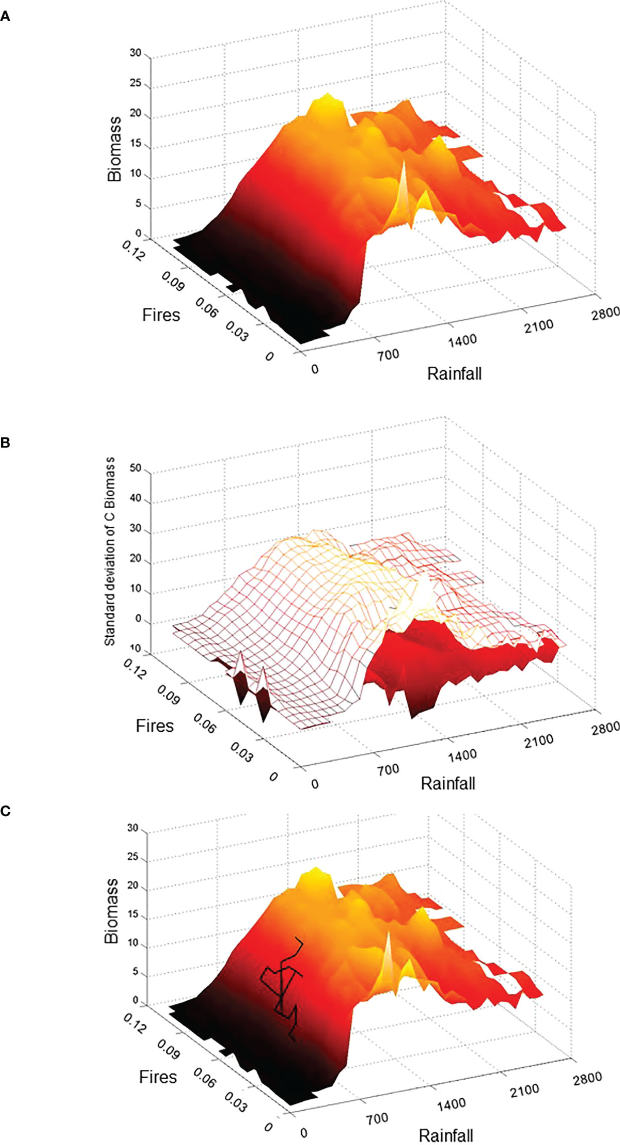
Figure 3 3D-representation of the tropical domain through the system Drape based on rasterized bin average biomass values (A) and its thickness (i.e. mean ± 1σ) (B). Axes units relate to annual Rainfall (in mm.year−1), vegetation carbon Biomass (in kg C.m−2), and Fire frequency (i.e. number of fires year−1). A hypothetical trajectory has been superimposed on the Drape for illustrative purpose (C). This trajectory could represent a geographical site and its lacustrine paleoecological reconstruction over the last 9000 years for climate (e.g., based on diatoms, chironomids, speleothems…), fires (e.g. micro-carbons), and vegetation (e.g., pollen, phytoliths, biomarkers…). We could project the chronological states obtained on the Drape, which would constitute the trajectory of this site and we could therefore follow this trajectory to highlight periods when the site has been in a stable state (homogeneous region see Figure 4) or inversely when its dynamics has experienced a major modification symbolized by the passage of the trajectory in a gradient or ridge zone (see Figure 4 for stable and unstable state detection).
The Drape is not a potential function, but it is associated with all possible types rather than with any specific catastrophe type. The computation of the Z-variable variance allows the capture of the inherent variability of the third ecosystem state-variable (the vegetation in Figure 3B) relative to the other two. Compared to the potential landscape from previous studies (Hirota et al., 2011; Scheffer et al., 2012), the neighborhood of each geographical location is lost in our proposed domain and Drape, other than that a location’s neighborhood is partially preserved in the spatial autocorrelation of the soil type (Supplementary Figure S2) and climate input data in the DGVM.
2.2 Analysis of the Drape: towards system states, resilience and trajectory understanding
Through the analysis of its heterogeneity, the Drape concept provides rich insights about a particular ecosystem or a biome shift. Using multiscale textural analysis (e.g. Gaucherel, 2007) on a 2D projection of the Drape (Figure 4A, similar to Figure 3A) produces a Drape heterogeneity map (Figure 4B) that can help detect different behaviors of the system. The heterogeneity index used is the evenness diversity index (see Supplementary information S1.2 for details of the computation). The higher the evenness diversity, the more heterogeneous the neighbor pixels on the map. Heterogeneous areas are therefore defined as having a high degree of evenness diversity amongst neighboring pixels (Figure 4B) highlighting statistically significant differences in the averaged biomass between neighboring pixels on the Drape (Figure 4A). Homogeneous areas (plateaus and valleys where neighboring pixels have low relative evenness diversity values) imply stable states and potential basins of attraction to explore through additional tests.
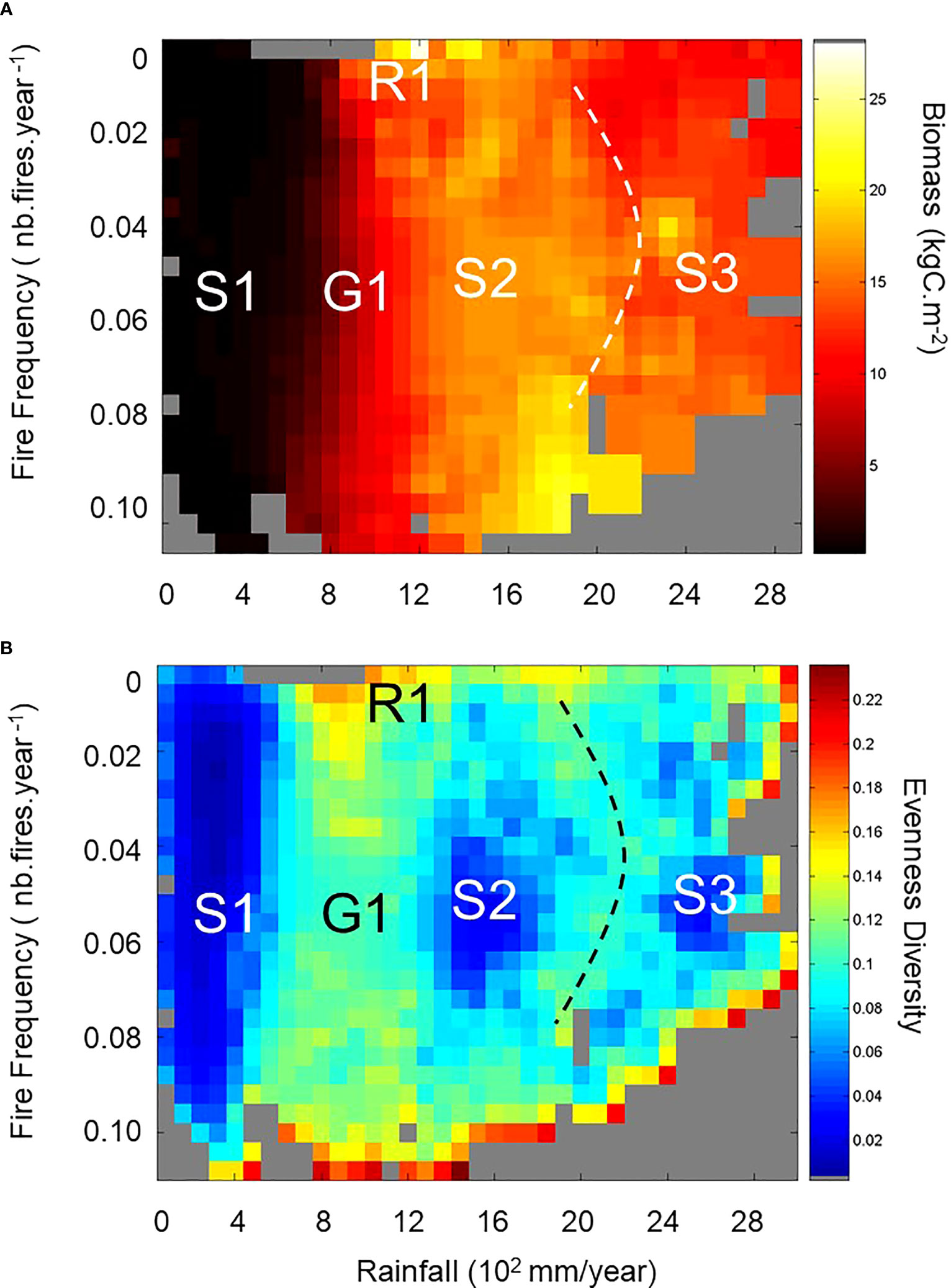
Figure 4 Analysis of the African Drape. (A) presents the Drape projection in the Rainfall–Fire plane. Note the position of the first bin (no fire, no rainfall) in the upper left corner compared to its position in the lower forward corner on Figure 3A, 3C. Here panel (A) also reports the projected stable and unstable states found with the textural analysis and highlighted in (B). Grey pixel areas could correspond with other tropical continental conditions (Southern America, Indonesia, Australia) not found currently in Africa, or with past conditions from which there is no present-day analogue condition. (B) shows the spatially explicit heterogeneity index (i.e., evenness diversity) resulting from the textural analysis based on the MHM method (see Supplementary information S1.2 and Gaucherel (2007)). The higher the index, the more heterogeneous the neighboring pixels on the multiscale map. Three stable (homogeneous – low evenness diversity with dark blue colors) and two unstable (heterogeneous – from light blue-yellow to red colors) state regions are highlighted. Grey areas on both panels represent non-existing system states based on the modern condition simulation. Note that red pixels, located on the lower and right edges of the plan in (B) result from edge effect computations due to poorly filled pixels and empty neighbouring pixels. We do not consider them as real heterogeneous pixels.
This heterogeneity analysis may seem to be in the same spirit as methods applied for the case of potential landscapes. An increased variance in Z associated with a small change in X or Y, measured as Drape heterogeneity, has utility to distinguish among stable (homogeneous zones), transient (gradients) and unstable (narrow ridges or peaks) behaviors (Briske et al., 2010). Such state characteristics result from the Drape’s topography, and not from the dataset value distribution as in the potential landscape concept (Hirota et al., 2011; Scheffer et al., 2012).
2.3 Use of the Drape to test ecological hypotheses
Beyond the presentation of the Drape, the objectives of this study were threefold. The first objective was to test whether the 600–1000 mm.yr−1 rainfall range, first proposed to discriminate closed-canopy forests from savannas (Sankaran et al., 2005), could be characterized on the Drape as a specific area such as a ridge or gradient). The second objective was to see whether several savanna types could be highlighted on the Drape due to climate–fire interactions (Hirota et al., 2011; Staver et al., 2011a; Favier et al., 2012) and whether these different types of savanna qualified as different stable states. Finally, the third objective was to test whether savanna and forest stable states would be found close enough to each other on the Drape to be considered as likely, adjacent alternative system states.
We used the dataset from Ruesh and Gibbs (2008) and their reporting of observed ranges of biomass based on climatic zones (IPCC, 2006), Global Ecofloristic Zones (FAO, 2001), and the Global Land Cover 2000 ecosystem classification (Bartholomé and Belward, 2005) to compare with the Drape value ranges.
3 Results and discussion
3.1 From the study-case: African ecosystems and states, and insights from the Drape for ecological hypotheses
The African Drape analysis using the Multiscale Heterogeneity Map method and the computation of the evenness diversity index revealed three homogeneous areas (namely S1, S2, S3 in Figure 4B) that we interpret as stable states, and two heterogeneous areas (the G1 gradient area interpreted as a transient state and the R1 ridge area interpreted as an unstable state in Figure 4B). Based on their African geographic locations (Supplementary Figure S3), we compared the characteristics of each revealed Drape area with those from the compiled observations (Ruesh and Gibbs, 2008) for precipitation, biomass, and ecosystem types (Table 1).
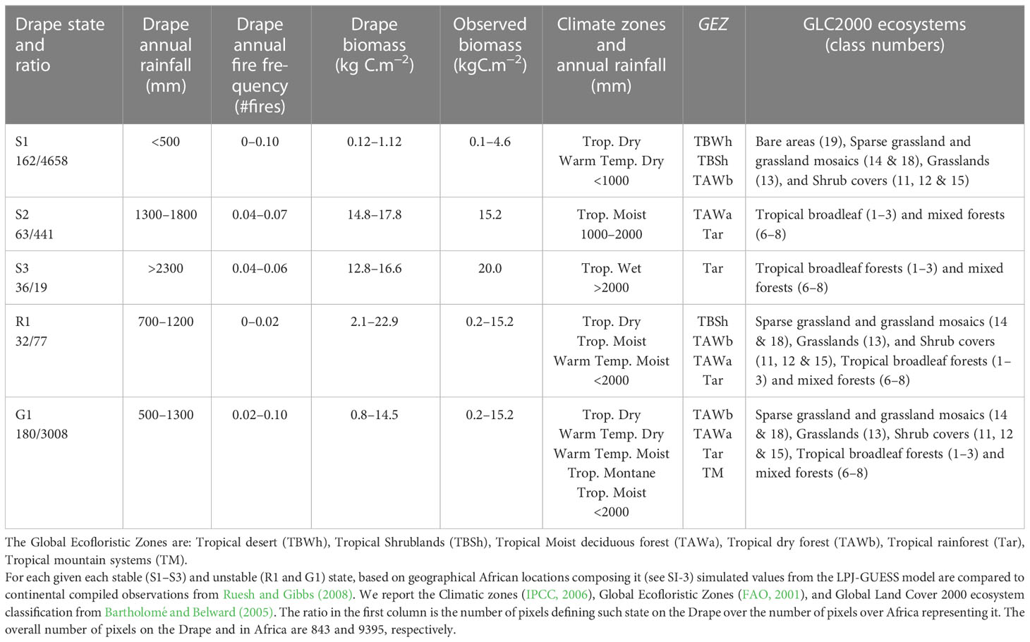
Table 1 Characteristics of stable and unstable African state regions revealed from the Drape textural analysis (Figure 4).
The S1 stable state (Figure 4B) represents the most arid regions with the lowest biomass range (Figure 4A; Table 1). Such characteristics and their associated geographic locations extracted from the LPJ-GUESS simulation (Supplementary Figure S3A), are in agreement with ecosystems from sparse grasslands to shrub-dominated savannas. The S1 biomass range likely matches the lower third of the observed range, because the S1 woody components represent less than 30% (not shown) of the potential C biomass simulated. S1 represents a stable state (a valley) on the Drape constituted by arid and semi-arid grassy biomes. They range from desert to tropical steppes to savannas with low woody cover.
The S2 stable state (Figure 4B) represents a plateau composed of regions with 1300–1800 mm annual rainfall, intermediate fire frequencies, and C biomass that is at least ten times heavier than that found in S1. These characteristics and their geographic locations (Supplementary Figure S3B) match perfectly with the tropical moist deciduous forest and rainforest (Table 1).
The S3 stable state (Figure 4B) having biomass range similar to that of S2 and with more than 2300 mm annual rainfall, is a plateau typified by rainforests (Supplementary Figure S3C). Simulated and observed characteristics of these locations conform with the African tropical wet climate regions (Table 1). While simulated biomasses are slightly lower than the mean observed, their range (Table 1) is in agreement with the full range (8.5–33 kgC.m−2) of observed rainforest biomasses. Note that vegetation models predict potential vegetation, so that slightly higher biomass than observed biomass is expected – even from reserves such as national parks in which low intensity management activities still exist.
Among the heterogeneous areas revealed by the multiscale map, R1 represents the most heterogeneous area even after discarding outlier pixels (Figure 4B). We describe the R1 area as a ridge because over such small extent area on the multiscale map of the Drape, characterized by a narrow range of quasi inexistent fires and a 700–1200 mm.yr−1 rainfall range, the simulated biomass range is the widest recorded (Figure 4A; Table 1, and Supplementary Figure S3D). This may be partly explained by the rainfall range that crosses the 1000 mm.yr−1 threshold discriminating tropical dry from tropical moist climates (Table 1). Consequently, these geographic areas include several ecosystems from sparse grasslands to tropical moist deciduous forests and rainforests whose observed biomasses, ranging from 0.2 to 15.2 kgC.m−2, agree well with the wide range extracted from the Drape (Table 1). The last large heterogeneous area is the G1 area, squeezed between S1 and S2 areas on the multiscale map (Figure 4B). G1 is a gradient representative of regions with a slightly wider rainfall range (500–1300 mm.yr−1) than that of R1, a wide range of fire occurrences, and as a consequence with a quite wide range of biomasses (Figure 4A; Table 1) but narrower than that of R1. Simulated characteristics and locations of G1 conditions (Table 1; Supplementary Figure S3E) include regions that are similar to those of R1 and mountain regions. Actually, the R1 ridge could also be considered as the most extreme conditions of the G1 gradient (see Supplementary Figure S3D), where heterogeneity is so high that the system switches from transient states along G1 to unstable states in the R1 area. It is worth noting that African regions composing the G1 transient states (alone or even associated with the R1 regions) are very similar to the regions classified as the projected worst-case biome changes expected in Africa over the 2071–2100 period as compared to the 1961–1990 reference (Niang et al., 2014). Finally, one could also see on the multiscale map a second gradient (dashed line on Figure 4), squeezed between S2 and S3 areas, but narrower and weaker than G1.
Based on these results, we confirm the first hypothesis since the 600–1000 mm.yr−1 rainfall range actually belongs to the G1 gradient that we consider as a transient state area, and to the R1 ridge that we consider as an unstable state occurring in the quasi absence of fires. However, we must reject the second and the third hypotheses because there is no stable state (homogeneous area) within this 600–1000 mm.yr−1 gradient that could be representative of any savanna stable state (second hypothesis), and in turns, the savanna-forest dynamics cannot be considered as alternative stable states. Conversely, we showed that S2 and S3 stable state areas represent different forest stable states and that part of the S1 stable state pixels may represent savannas with low woody cover (less than 30% of the very light biomass (<1.5 kgC.m−2)). However, these stable savannas grow with less than 500 mm.yr−1 in rainfall, which is at least 2.6 and 4.6 times drier than annual rainfall for S2 and S3, respectively.
Several paleoecological studies have shown that during the Holocene African Humid Period (de Menocal et al., 2000) and the so-called “Green Sahara” (Chikira et al., 2006; Watrin et al., 2009), several paleolakes were present in the current Saharan and Sahelian regions (Lézine et al., 2011). This was a response to intensified monsoonal rainfall that penetrated inland more than 10° northwards. The rainbelt core migrated up to 5° northwards during the humidity optimum (Texier et al., 2000). Such moister conditions over the 15–20°N latitudinal region, as compared to its present-day aridity, created good environmental conditions for the Guinean-Congolian pollen taxa (Hély et al., 2014) that are exclusively representative of modern tropical rainforest. This suggests that some geographic locations have therefore experienced ecosystem or even biome shifts over the last millennia that may have been similar to those from the S1 to S2 and/or to S3 stable states. Further research is needed to assess the speed of these past changes, to plot geographic-site trajectory on the Drape (as conceptually illustrated on Figure 3C), and to apprehend paths and likely direction shifts.
The multiscale map analysis suggests that most savannas (i.e. GLC2000 forest mosaic and shrub cover classes with 5.0–10.0 kgC.m−2 biomass range (Ruesh and Gibbs, 2008)) lie on the G1 gradient area and are therefore transient states but without delimited stable states. These savannas could shift to R1 unstable states if only fire (or a similar disturbance such as grazing (Bond et al., 2005) would almost disappear, while they could shift to S2 (S1) stable states if only rainfall would increase (decrease), and only to S1 if both rainfall would decrease and fire would change. Past savanna dynamics applied on the Drape could provide insights on past realized-trajectories and speed. The overall Drape information could be useful for savanna-ecosystem sustainable management, for instance to avoid bush-encroachment (Ringrose et al., 1998) that one could consider as a shift to R1 conditions.
Once valleys (S1) and plateaus (S2 and S3) are identified on the Drape, their location, width and depth could quantify the importance of these basins of attraction, such characterization corresponding well with the system resilience as defined by Walker et al. (2004) and discussed by Beisner et al. (2003) for ecosystem management perspectives. Similarly, ridges could represent the boundaries of contiguous basins of attraction. As previously noted, ridges could be interpreted as bifurcation states (i.e. tipping points) from which small changes in the state variables would induce an ecosystem shift or even a biome shift. From the location (state) of the system on these Drape areas, one could also estimate objectively the latitude (i.e. width) and the resistance (i.e. depth) of the basin of current ecosystems, as well as its precariousness (i.e. its distance to the ridge, which is the boundary of the basin of attraction) and its likely resilience as suggested by Beisner et al. (2003) and Walker et al. (2004).
Observations from current conditions, from past reconstructions or from future projections based on different socio-economic and climatic scenarios can provide the realized states found in different areas of the Drape. Analysis of an ecosystem at a given geographical location and its trajectory on the Drape could provide expected temporal changes of the state variables. One could therefore analyze and validate the Drape variations (i.e. its topography) from embedded system trajectories reconstructed from observations and/or paleoecological studies as conceptually illustrated in Figure 3C.
3.2 Benefits of the Drape concept
Understanding ecosystem dynamics as a scientific objective and predicting future responses as a more practical objective are difficult tasks. We propose departing from the current methods based on differential equation systems and/or statistical approaches, as well as from simplifications of the abiotic and disturbance components of ecosystems. Because our method only relies on observed data for validation, one avoids misinterpretation. Debates concerning possible extrapolation in cases of slow dynamics (as suggested above) should move toward synthesis (e.g. Hirota et al., 2011; Ratajczak and Nippert, 2012). The proposed Drape concept is an improvement in ecosystem understanding for the following seven reasons:
i) The Drape presents in a single multidimensional space all ecosystems governed by the same first-order state variables and allows to position and characterize the different states of these ecosystems in order to later study past, present, or future trajectories. (Figure 2 and Supplementary information S1.1). This process-based approach will allow including ecosystem responses over long periods of time and through several spatial (from local to continental) scales. This satisfies the need to retrieve slow but integrative changes during regime shifts that may appear incremental at human time scales (Ratajczak and Nippert, 2012; Hughes et al., 2013b). For example, the response to global warming by terrestrial ecosystems at the end of the last ice age (Minckley et al., 2012) or at the end of the African Humid Period (Lézine et al., 2011; Hély et al., 2014) took millennia, long after the ice sheets had melted or after the African monsoon intensification had terminated.
ii) The Drape, built from the outputs of the process-based model, includes disturbances as a state variable as important as vegetation or precipitation and thus allows to better characterize each ecosystem, its states, and its functional neighbors. Indeed, disturbances were previously considered as parameters or external forces in the representation of system dynamics and manifested an effect on the ecosystem through the biotic component only (e.g. Staver et al., 2011b; Touboul et al., 2018). By definition, ecosystems are simultaneously biotic and abiotic, with several tightly interacting components (e.g. flora, fauna, soils, atmosphere and humans). There is no conceptual reason to focus on a specific component over the others (Gignoux et al., 2011; Schwartz and Jax, 2011; Gaucherel, 2014). This matches the observation that ecosystems are simultaneously conditioned by the laws of thermodynamics and the by natural selection.
iii) The state variables used to build the space and the Drape are symmetric in the system functioning. Each axis has the same weight and equal role in constructing the domain (Figure 2). With this property in mind, the 3D space is the smallest multidimensional space aiming at synthetizing any ecosystem state. More complicated domains can take into account additional extra state variables (e.g. human activities or fauna), if required (Cincotta et al., 2000). The symmetry between state variables also allows the study of the system and its states from different points of view (Figures 2A, B), while maintaining the mechanistic relationships among the state variables.
iv) The Drape itself provides an instantaneous and convenient visualization of the different states encountered, as well as their characterization in terms of associated state variable values. This is interpreted in the example case as an averaged and rasterized (grid-based) surface (Figures 3, 4) of the realized domain (Figure 2).
v) The textural analysis explores the Drape variations to identify basins of attraction, characteristic tipping points and their relationships in terms of distance (Figure 4; Appendix 2). Using a statistical moment such as the mean to build the Drape surface prevents from finding “folded backward” regions previously considered as tipping-points or induced catastrophic shifts (Scheffer et al., 2001). However, tipping-points on the Drape are materialized as ridges (i.e. most heterogeneous areas, Figure 3A). Once identified and delineated, the analysis informs the possible system behavior further away. Methods other than the multiscale textural analysis shown here may be used to analyze the Drape, such as a spectral analysis (e.g. Keitt, 2000).
vi) The Drape concept is generic. It allows featuring all states and associated state variables values extracted from a process-based model. The Drape concept could therefore be used to study other terrestrial, marine, or fresh water ecosystems as long as the chosen state variables are the best representative ones and that values are extracted from (state-of-the-art) process-based model. The Drape can be used for different periods than nowadays, which may point to states being located in different areas of the Drape as compared to the present-day state.
vii) By reporting onto the Drape the trajectory a given geographical location would record through time (observed from time-series such as remote-sensing datasets, simulated from process-based models, or reconstructed from paleoecological datasets, see Figure 3C) we would visualize and analyze its dynamics and clearly characterize the states it went through. Despite its resemblance with real topography or a Waddington’s landscape (Goldberg et al., 2007), it is worth emphasizing that the third axis (Z) of the domain does not carry the meaning of a vertical and oriented direction such as the one constrained by gravity (e.g. Scheffer et al., 2001; Beisner et al., 2003). On this Drape, a ball representing the ecosystem state at a specific location and time could easily move up to higher Z values due to any ecological process. As such, the Drape surface appears much more similar to a chaotic manifold (further discussed below) than the stability landscape of the potential mentioned in previous studies. The Drape surface also seems to combine the ecosystem and the community perspectives from Beisner et al. (2003). Indeed, no process directly acts on this ball (i.e. the ball is not pushed by an external force), but rather intrinsic and stochastic processes modify one or several state variable values which, in turn, “push” the system toward another area of the Drape (Abarbanel, 1996; Strogatz, 2001). Moreover, basins of attraction are not systematically the lowest Drape areas.
In practice, a different domain (and its associated Drape) should be recomputed whenever a state variable should be replaced by another more important or representative variable. This allows different neighboring ecosystems (or even biomes) to occur within the same domain, and approximated by a common Drape. It seems reasonable to find tropical forest and savanna biomes in the same domain, but boreal biomes (e.g. coniferous forests and tundra) would be in another distinct domain, as they would require different ecosystem state variables (e.g. temperature instead of precipitation). This should also allow identifying past ecosystem states for which there are no modern analogues (e.g. the “green Sahara” during the mid-Holocene) in specific areas of the Drape (e.g. Figure 4B, lower right region, which is currently empty). Every biome observed during a given period will likely not occupy all of its potential Drape area. So, the Drape concept does not fully solve the problem of defining the ecosystem or biome boundaries (Gignoux et al., 2011; Gaucherel, 2014). The limits, here defined by the extreme values of each state variable, are physically constrained, while a priori the Drape extent is not. Such boundaries would simultaneously depend on the maximum system variability and by the addressed question.
The Drape concept applied to ecosystems can play an important role in the tipping point debate (Ratajczak and Nippert, 2012; Brook et al., 2013; Gaucherel and Moron, 2015). With tipping points defined as sharp changes in ecosystem dynamics, such changes would fit with all sharp gradients (clines) and sharp peaks observed in the Drape variations. Indeed, to shift from a relatively smooth or flat (i.e. homogeneous) area of the Drape to another one by a sharp gradient is a clue of abrupt variations in states (Lenton et al., 2008; Kriegler et al., 2009). Such tipping points could easily be identified and quantified on the Drape based on their sharpness (relatively to other zones) and from their direction.
In our African example, the G1 gradient appeared approximately twice as heterogeneous as its neighboring stable states (S1 and S2) assimilated to steppes-grassy savannas and forest types, respectively, based on state variable values (Figure 4A). We stress that such transitions are not necessary “state transitions” such as those observed in chaotic systems (Abarbanel, 1996; Ghil et al., 2002), and they would definitely need a detailed and rigorous mathematical analysis to be demonstrated as attempted in some recent studies (Accatino et al., 2010; Zaliapin and Ghil, 2010).
3.3 Limitations of the domain and perspectives
The limitations of the Drape concept presented here are of two sorts. First, there are methodological limitations, which hopefully can be improved upon and progressively removed. For instance, the variability arising from similar geographic areas (i.e. close points in the domain) probably contributes to the volume or “thickness” of the realized domain (Figure 3B). This variability may be retrieved by the calculation and representation of another statistical moment (e.g. variance) of the domain, and be analyzed in a similar manner than the averaged Drape (Figure 4). Moreover, using different moments or statistics such as the mode would allow representation of bimodal distributions in each (X, Y) interval bin if they exist, and thus to the plotting of more complicated (e.g. folded) Drape variations. Such complicated responses have been studied in detail in the catastrophe theory (e.g. the cusp geometry (Thom, 1972)), and ecological studies would gain in applying such a rigorous analysis to ecosystems (Gaucherel et al., 2020).
For clarity, we did not explore the specific role of human beings as one of the ecosystem components. As with other unmentioned ecosystem components (e.g. soils), humans could partly be involved as part of one of the already included components (e.g. climate and/or fires), or as an additional component. The resultant four-dimensional space and the more complicated 3D-Drape (called a hypersurface) could be treated without technical difficulties. This is obviously useful for applied questions related to ecosystem management and environmental policies, and it would be relevant to explore this possibility in human-perturbed systems (Cincotta et al., 2000; Gaucherel et al., 2012).
The second category of limitations of the Drape concept involves the effort needed ultimately to represent a more functional concept such as ecosystem chaos. The Drape concept carries on the ecosystem trajectory that follows the Drape response surface from the spatial and temporal autocorrelations of system components (Figure 3C). With the exception of ridge areas and other possible singularities, each ecosystem state globally shows a high correlation with the next (and nearby) state (Figure 4), due to the processes involved and function of model equations (e.g. Cramer et al., 1999; Smith et al., 2001; Sitch et al., 2008), as well as due to the spatial autocorrelation in the abiotic state variables.
It would be convenient and parsimonious to build the Drape with the system trajectories themselves, which is the approach that provides the dynamical system theory and chaotic system representations in previous studies (Lorenz, 1963; Takens, 1981). To write and solve the equations for a dynamical system would directly lead to a trajectory in the phase-space. This approach assumes that ecosystems are dynamical and possibly chaotic, i.e. fully deterministic, ergodic and sensitive to small variations in initial conditions (Lorenz, 1963; Strogatz, 2001). To our knowledge, this has never been demonstrated for an ecosystem as a whole, although it is documented for some components such as prey–predator subsystems (May, 1977), vegetation dynamics (Solé and Bascompte, 2006) or climate dynamics (e.g. Ghil et al., 2002). However, a focus on purely biotic (or abiotic) components omits the necessary symmetry between biotic, abiotic and disturbance components (e.g. Gaucherel et al., 2020). This is the spirit of the present study.
4 Conclusion
We propose and illustrate a new and potentially powerful concept to capture ecosystem dynamics and the related complexity. With a Drape structure embedded into a multidimensional space made up with biotic, abiotic and disturbance state variables, the representation provides a simplification of ecosystem dynamics into a smoothed, quantitative and intuitive representation. It is our hope that the Drape concept and its associated properties, which are borrowed from dynamic system theory and catastrophe theory, will facilitate understanding, visualization and prediction of ecosystem dynamics. The Drape concept is a next step in the direction of analytically demonstrating the complex and possibly chaotic behaviors commonly assumed for ecosystems. It needs to be tested and validated based on further observations and simulations. We fully expect that it will prove useful for further exploration of ecosystem functioning and tipping-point related issues.
Data availability statement
The raw data supporting the conclusions of this article will be made available by the authors, without undue reservation.
Author contributions
CH and CG designed the research, CH provided data and CG performed the textural analysis. CH, CG, RS and HS discussed the results, and CH wrote the first draft of the manuscript. All authors contributed to the article and approved the submitted version.
Acknowledgments
This work has been performed in the framework of the French Labex CeMEB. We warmly thank Samuel Alleaume for proposing the “Drape” term to pinpoint this milestone concept.
Conflict of interest
The authors declare that the research was conducted in the absence of any commercial or financial relationships that could be construed as a potential conflict of interest.
Publisher’s note
All claims expressed in this article are solely those of the authors and do not necessarily represent those of their affiliated organizations, or those of the publisher, the editors and the reviewers. Any product that may be evaluated in this article, or claim that may be made by its manufacturer, is not guaranteed or endorsed by the publisher.
Supplementary material
The Supplementary Material for this article can be found online at: https://www.frontiersin.org/articles/10.3389/fevo.2023.1108914/full#supplementary-material
References
Accatino F., De Michele C., Vezzoli R., Donzelli D., Scholes R. J. (2010). Tree–grass co-existence in savanna: interactions of rain and fire. J. Theor. Biol. 267, 235–242. doi: 10.1016/j.jtbi.2010.08.012
Adler P. B., Levine J. M. (2007). Contrasting relationships between precipitation and species richness in space and time. Oïkos 116, 221–232. doi: 10.1111/j.0030-1299.2007.15327.x
Aleman J., Blarquez O., Bentaleb I., Bonté P., Brossier B., Carcaillet C., et al. (2013). Tracking land-cover changes with sedimentary charcoal in the afrotropics. Holocene 23, 1853–1862. doi: 10.1177/0959683613508159
Aleman J. C., Fayolle A., Favier C., Staver A. C., Dexter K. G., Ryan C. M., et al. (2020). Floristic evidence for alternative biome states in tropical Africa. Proc. Natl. Acad. Sci. U.S.A. 117, 28183–28190. doi: 10.1073/pnas.2011515117
Ali A. A., Blarquez O., Girardin M. P., Hély C., Tinquaut F., El Guellab A., et al. (2012). Control of the multimillennial wildfire size in boreal north America by spring climatic conditions. Proc. Natl. Acad. Sci. 109, 20966–20970. doi: 10.1073/pnas.1203467109
Archer S. (1989). Have southern texas savannas been converted to woodlands in recent history? Am. Nat. 134, 545–561. doi: 10.1086/284996
Bartholomé E., Belward A. S. (2005). GLC2000: a new approach to global land cover mapping from earth observation data. Int. J. Remote Sens. 26, 1959–1977. doi: 10.1080/01431160412331291297
Beisner B. E., Haydon D. T., Cuddington K. (2003). Alternative stable states in ecology. Front. Ecol. Environ. 1, 376–382. doi: 10.1890/1540-9295(2003)001[0376:ASSIE]2.0.CO;2
Bel G., Hagberg A., Meron E. (2012). Gradual regime shifts in spatially extended ecosystems. Theor. Ecol. 5, 591–604. doi: 10.1007/s12080-011-0149-6
Blois J. L., Williams J. W., Fitzpatrick M. C., Jackson S. T., Ferrier S. (2013). Space can substitute for time in predicting climate-change effects on biodiversity. Proc. Natl. Acad. Sci. 110, 9374–9379. doi: 10.1073/pnas.1220228110
Boettiger C., Ross N., Hastings A. (2013). Early warning signals: the charted and uncharted territories. Theor. Ecol. 6, 255–264. doi: 10.1007/s12080-013-0192-6
Bond W. J., Woodward F. I., Midgley G. F. (2005). The global distribution of ecosystems in a world without fire. New Phytol. 165, 525–537. doi: 10.1111/j.1469-8137.2004.01252.x
Boulton C. A., Good P., Lenton T. M. (2013). Early warning signals of simulated Amazon rainforest dieback. Theor. Ecol. 6, 373–384. doi: 10.1007/s12080-013-0191-7
Briske D. D., Washington-Allen R. A., Johson C. R., Lockwood J. A., Lockwood D. R., Stringham T. K., et al. (2010). Catastrophic thresholds: a synthesis of concepts, perspectives, and applications. Ecol. Soc. 15. doi: 10.5751/ES-03681-150337
Brook B. W., Ellis E. C., Perring M. P., Mackay A. W., Blomqvist L. (2013). Does the terrestrial biosphere have planetary tipping points? Trends Ecol. Evol. 28, 396–401. doi: 10.1016/j.tree.2013.01.016
Carpenter S., Walker B., Anderies J. M., Abel N. (2001). From metaphor to measurement: resilience of what to what? Ecosystems 4, 765–781. doi: 10.1007/s10021-001-0045-9
Chapin F. S. I., Callaghan T. V., Bergeron Y., Fukuda M., Johnstone J. F., Juday G., et al. (2004). Global change and the Boreal forest: thresholds, shifting states or gradual change? Ambio 33, 361–365. doi: 10.1579/0044-7447-33.6.361
Chaste E., Girardin M. P., Kaplan J. O., Portier J., Bergeron Y., Hély C. (2018). The pyrogeography of eastern boreal Canada from 1901 to 2012 simulated with the LPJ-LMfire model. Biogeosciences 15, 1273–1292. doi: 10.5194/bg-15-1273-2018
Chikira M., Abe-Ouchi A., Sumi A. (2006). General circulation model study on the green Sahara during the mid-Holocene: an impact of convection originating above boundary layer. J. Geophysical Res. 111. doi: 10.1029/2005JD006398
Cincotta R. P., Wisnewski J., Engelman R. (2000). Human population in the biodiversity hotspots. Nature 404, 990–992. doi: 10.1038/35010105
Conversi A., Dakos V., Gardmark A., Ling S., Folke C., Mumby P. J., et al. (2015). A holistic view of marine regime shifts. Philos. Trans. R. Soc. B-Biological Sci. 370. doi: 10.1098/rstb.2013.0279
Cramer W., Kicklighter D. W., Bondeau A., Moore B. III, Churkina G., Nemry B., et al. (1999). Comparing global models of terrestrial net primary productivity (NPP): overview and key results. Global Change Biol. 5, 1–15. doi: 10.1046/j.1365-2486.1999.00009.x
Dakos V., Carpenter S. R., Brock W. A., Ellison A. M., Guttal V., Ives A. R., et al. (2012). Methods for detecting early warnings of critical transitions in time series illustrated using simulated ecological data. PloS One 7. doi: 10.1371/journal.pone.0041010
Dakos V., Scheffer M., van Nes E. H., Brovkin V., Petoukhov V., Held H. (2008). Slowing down as an early warning signal for abrupt climate change. Proc. Natl. Acad. Sci. United States America 105, 14308–14312. doi: 10.1073/pnas.0802430105
Dakos V., van Nes E. H., Donangelo R., Fort H., Scheffer M. (2010). Spatial correlation as leading indicator of catastrophic shifts. Theor. Ecol. 3, 163–174. doi: 10.1007/s12080-009-0060-6
Dakos V., van Nes E. H., Scheffer M. (2013). Flickering as an early warning signal. Theor. Ecol. 6, 309–317. doi: 10.1007/s12080-013-0186-4
Davis M. B., Shaw R. G. (2001). Range shifts and adaptative responses to quaternary climate change. Science 292, 673–679. doi: 10.1126/science.292.5517.673
de Menocal P., Ortiz J., Guilderson T., Adkins J., Sarnthein M., Baker L., et al. (2000). Abrupt onset and termination of the African humid period: rapid climate responses to gradual insolation forcing. Quaternary Sci. Rev. 19, 347–361. doi: 10.1016/S0277-3791(99)00081-5
D’Odorico P., Laio F., Ridolfi L. (2005). Noise-induced stability in dryland plant ecosystems. Proc. Natl. Acad. Sci. 102, 10819–10822. doi: 10.1073/pnas.0502884102
Drukenbrod D. L., Martin-Benito D., Orwig D. A., Pederson N., Poulter B., Renwick K. M., et al. (2019). Redefining temperate forest responses to climate and disturbance in the eastern united states: new insights at the mesoscale. Global Ecol. Biogeography 28, 557–575. doi: 10.1111/geb.12876
Dutta P. S., Sharma Y., Abbott K. C. (2018). Robustness of early warning signals for catastrophic and non-catastrophic transitions. Oïkos 127, 1251–1263. doi: 10.1111/oik.05172
Ellis J. E., Swift D. (1988). Stability of African pastoral ecosystems: alternate paradigms and implications for development. J. Range Manage. 41, 450–459. doi: 10.2307/3899515
FAO (2001). Global forest resources assessment 2000 (Rome: Food and Agriculture Organization of the United Nations).
Favier C., Aleman J., Bremond L., Dubois M. A., Freycon V., Yangakola J.-M. (2012). Abrupt shifts in African savanna tree cover along a climatic gradient. Global Ecol. Biogeography 21, 787–797. doi: 10.1111/j.1466-8238.2011.00725.x
Folke C., Carpenter S., Walker B., Scheffer M., Elmqvist T., Gunderson L., et al. (2004). Regime shifts, resilience, and biodiversity in ecosystem management. Annu. Rev. Ecology Evolution Systematics 35, 557–581. doi: 10.1146/annurev.ecolsys.35.021103.105711
Gaucherel C. (2007). Multiscale heterogeneity map and associated scaling profile for landscape analysis. Landscape Urban Plann. 82, 95–102. doi: 10.1016/j.landurbplan.2007.01.022
Gaucherel C. (2014). Ecosystem complexity through the lens of logical depth: capturing ecosystem individuality. Biol. Theory 9, 440–451. doi: 10.1007/s13752-014-0162-2
Gaucherel C., Alleaume S., Hély C. (2008). The comparison map profile method: a statistical tool for spatially explicite and multiscale comparison of quantitative and qualitative images. IEEE Geosci. Remote Sens. Lett. 46, 2708–2719. doi: 10.1109/TGRS.2008.919379
Gaucherel C., Boudon F., Houet T., Castets M., Godin C. (2012). Understanding patchy landscape dynamics: towards a landscape language. PloS One 7, e46064. doi: 10.1371/journal.pone.0046064
Gaucherel C., Moron V. (2015). Potential stabilizing points to mitigate tipping point interactions in earth’s climate. Int. J. Climatology. doi: 10.1002/joc.4712
Gaucherel C., Pommereau F., Hély C. (2020). Understanding ecosystem complexity via application of a process-based state space rather than a potential. Complexity. doi: 10.1155/2020/7163920
Ghil M., Allen M. R., Dettinger M. D., Ide K., Kondrashov D., Mann M. E., et al. (2002). Advanced spectral methods for climatic time series. Rev. Geophysics 40, 3-1-3–3-141. doi: 10.1029/2000RG000092
Gignoux J., Davies I. D., Flint S. R., Zucker J.-D. (2011). The ecosystem in practice : interest and problems of an old definition for constructing ecological models. Ecosystems 14, 1039–1054. doi: 10.1007/s10021-011-9466-2
Goldberg A. D., Allis C. D., Bernstein E. (2007). Epigenetics: a landscape takes shape. Cell 128, 635–638. doi: 10.1016/j.cell.2007.02.006
Hanan N. P., Tredennick A. T., Prihodko L., Bucini G., Dohn J. (2014). Analysis of stable states in global savannas: is the CART pulling the horse? Global Ecol. Biogeography 23, 259–263. doi: 10.1111/geb.12122
Hanan N. P., Tredennick A. T., Prihodko L., Bucini G., Dohn J. (2015). Analysis of stable states in global savannas – a response to staver and Hansen. Global Ecol. Biogeography 24, 988–989. doi: 10.1111/geb.12321
Hély C., Braconnot P., Watrin J., Zheng W. (2009). Climate and vegetation : simulating the African humid period. Comptes Rendus Géoscience 341, 671–688. doi: 10.1016/j.crte.2009.07.002
Hély C., Bremond L., Alleaume S., Smith B., Sykes M. T., Guiot J. (2006). Sensitivity of African biomes to changes in the precipitation regime. Global Ecol. Biogeography 15, 258–270. doi: 10.1111/j.1466-8238.2006.00235.x
Hély C., Chaste E., Girardin M. P., Remy C., Blarquez O., Bergeron Y., et al. (2020). A Holocene perspective of vegetation controls on seasonal Boreal wildfire sizes using numerical paleo-ecology. Front. In Forests Global Change 3. doi: 10.3389/ffgc.2020.511901
Hély C., Girardin M. P., Ali A. A., Carcaillet C., Brewer S., Bergeron Y. (2010). Eastern Boreal north American wildfire risk of the past 7000 years: a model-data comparison. Geophysical Res. Lett. 37. doi: 10.1029/2010GL043706
Hély C., Lézine A. M., APD Contributors (2014). Holocene Changes in African vegetation: tradeoff between climate and water availability. Climate Past 10, 681–686. doi: 10.5194/cpd-9-6397-2013
Hickler T., Vohland K., Feehan J., Miller P. A., Smith B., Costa L., et al. (2012). Projecting the future distribution of European potential natural vegetation zones with a generalized, tree species-based dynamic vegetation model. Global Ecol. Biogeography 21, 50–63. doi: 10.1111/j.1466-8238.2010.00613.x
Hirota M., Holmgren M., Van Nes E. H., Scheffer M. (2011). Global resilience of tropical forest and savanna to critical transitions. Science 334, 232–235. doi: 10.1126/science.1210657
Holling C. S. (1973). Resilience and stability of ecological systems. Annu. Rev. Ecol. Systematics 4, 1–23. doi: 10.1146/annurev.es.04.110173.000245
Hughes T. P., Carpenter S., Rockström J., Scheffer M., Walker B. (2013a). Multiscale regime shifts and planetary boundaries. Trends Ecol. Evol. 28, 389–395. doi: 10.1016/j.tree.2013.05.019
Hughes T. P., Linares C., Dakos V., van de Leemput I. A., van Nes E. H. (2013b). Living dangerously on borrowed time during slow, unrecognized regime shifts. Trends Ecol. Evol. 28, 149–155. doi: 10.1016/j.tree.2012.08.022
IPCC (2006). “2006 guidelines for national greenhouse gas inventories,” in Agriculture, forest, and other land use, vol. 4. (Hayama, Japan: IGES).
Johnson E. A. (1992). Fire and vegetation dynamics: studies from the north American boreal forest (Cambridge: Cambridge University Press).
Kéfi S., Guttal V., Brock W. A., Carpenter S. R., Ellison A. M., Livina V. N., et al. (2014). Early warning signals of ecological transitions: methods for spatial patterns. PloS One 9, e92097 1–13. doi: 10.1371/journal.pone.0092097
Keitt T. H. (2000). Spectral representation of neutral landscapes. Landscape Ecol. 15, 479–493. doi: 10.1023/A:1008193015770
Kriegler E., Hall J. W., Held H., Dawson R., Schellnhuber H. J. (2009). Imprecise probability assessment of tipping points in the climate system. Proc. Natl. Acad. Sci. 106, 5041–5046. doi: 10.1073/pnas.0809117106
Lenton T. M., Held H., Kriegler E., Hall J. W., Lucht W., Rahmstorf S., et al. (2008). Tipping elements in the earth’s climate system. Proc. Natl. Acad. Sci. 105, 1786–1793. doi: 10.1073/pnas.0705414105
Lézine A.-M., Hély C., Grenier C., Braconnot P., Krinner G. (2011). Sahara And sahel vulnerability to climate changes, lessons from Holocene hydrological data. Quaternary Sci. Rev. 30, 3001–3012. doi: 10.1016/j.quascirev.2011.07.006
Livina V. N., Kwasniok F., Lenton T. M. (2010). Potential analysis reveals changing number of climate states during the last 60 kyr. Climate Past 6, 77–82. doi: 10.5194/cp-6-77-2010
Lorenz E. N. (1963). Deterministic nonperiodic flow. J. Atmospheric Sci. 20, 130–141. doi: 10.1175/1520-0469(1963)020<0130:DNF>2.0.CO;2
Martin R., Schlüter M., Blenckner T. (2020). The importance of transient social dynamics for restoring ecosystems beyond ecological tipping points. Proc. Natl. Acad. Sci. 117, 2717–2722. doi: 10.1073/pnas.1817154117
May R. M. (1977). Thresholds and breakpoints in ecosystems with a multiplicity of stable states. Nature 269, 471–477. doi: 10.1038/269471a0
McMahon S. M., Harrison S., Armbruster W. S., Bartlein P. J., Beale C. M., Edwards M. E., et al. (2011). Improving assessment and modelling of climate change impacts on global terrestrial biodiversity. Trends Ecol. Evol. 26, 249–259. doi: 10.1016/j.tree.2011.02.012
Minckley T. A., Shriver R. K., Shuman B. (2012). Resilience and regime change in a southern rocky mountain ecosystem during the past 17 000 years. Ecol. Monogr. 82, 49–68. doi: 10.1890/11-0283.1
New M. G., Lister D., Hulme M., Makin I. (2002). A high-resolution data set of surface climate over global land areas. Climate Res. 21, 1–25. doi: 10.3354/cr021001
Niang I., Ruppel O. C., Abdrabo M. A., Essel A., Lennard C., Padgham J., et al. (2014). “Africa,” in Climate change 2014: impacts, adaptation, and vulnerability. part b: regional aspects. contribution of working group II to the fifth assessment report of the intergovernmental panel on climate change. Eds. Barros V. R., Field C. B., Dokken D. J., Mastrandrea M. D., Mach K. J., Bilir T. E., et al (Cambridge, United Kingdom and New York, NY, USA: Cambridge University Press), 1199–1265.
Nolting B. C., Abbott K. C. (2016). Balls, cups, and quasi-potentials: quantifying stability in stochastic systems. Ecology 94, 850–864. doi: 10.1890/15-1047.1
Noy-Meir I. (1975). Stability of grazing systems: an application of predator-prey graphs. journal of ecology. J. Ecol. 63, 459–481. doi: 10.2307/2258730
Pickett S. T. A., White P. S. (1985). The ecology of natural disturbance and patch dynamics (Academic Press Inc. New york: Academic press).
Prentice I. C., Kelley D. I., Foster P. N., Friedlingstein P., Harrison S., Bartlein P. J. (2011). Modeling fire and the terrestrial carbon balance. Global Biogeochemical Cycles 25. doi: 10.1029/2010GB003906
Prentice I. C., Webb T. III (1998). BIOME 6000: reconstructing global mid-Holocene vegetation patterns from palaeoecological records. J. Biogeography 25, 997–1005. doi: 10.1046/j.1365-2699.1998.00235.x
Ratajczak Z., D’Odorico P., Collins S. L., Bestelmeyer B. T., Isbell F. I., Nippert J. B. (2017a). The interactive effects of press/pulse intensity and duration on regime shifts at multiple scales. Ecol. Monogr. 87, 198–218. doi: 10.1002/ecm.1249
Ratajczak Z., D’Odorico P., Nippert J. B., Collins S. L. (2017b). Changes in spatial variance during a grassland to shrubland state transition. J. Ecol. 105, 750–760. doi: 10.1111/1365-2745.12696
Ratajczak Z., Nippert J. B. (2012). Comment on “Global resilience of tropical forest and savanna to critical transitions.” Science 336, 541. doi: 10.1126/science.1219346
Ringrose S., Matheson W., Vanderpost C. (1998). Analysis of soil organic carbon and vegetation cover trends along the Botswana Kalahari transect. J. Arid Environments 38, 379–396. doi: 10.1006/jare.1997.0344
Ruesh A., Gibbs H. K. (2008). New IPCC tier-1 global biomass carbon map for the year 2000 (Oak Ridge, Tennessee: Oak Ridge National Laboratory). Available online from the Carbon Dioxide Information Analysis Center. Available at: http://cdiac.ess-dive.lbl.gov.
Sankaran M., Hanan N. P., Scholes R., Ratnam J., Augustine D. J., Cade B. S., et al. (2005). Determinants of woody cover in African savannas. Nature 438, 846–849. doi: 10.1038/nature04070
Scheffer M., Carpenter S., Foley J. A., Folke C., Walker B. (2001). Catastrophic shifts in ecosystems. Nature 413, 591–596. doi: 10.1038/35098000
Scheffer M., Hirota M., Holmgren M., Van Nes E. H., Chapin F. S. I. (2012). Thresholds for boreal biome transitions. Proc. Natl. Acad. Sci. 109, 21384–21389. doi: 10.1073/pnas.1219844110
Scheffer M., Holmgren M., Brovkin V., Claussen M. (2005). Synergy between small- and large-scale feedbacks of vegetation on the water cycle. Global Change Biol. 11, 1003–1012. doi: 10.1111/j.1365-2486.2005.00962.x
Scholes R. J., Dowty P. R., Caylor K., Parsons D. A. B., Frost P. G. H., Shugart H. H. (2002). Trends in savanna structure and composition along an aridity gradient in the Kalahari. J. Vegetation Sci. 13, 419–428. doi: 10.1111/j.1654-1103.2002.tb02066.x
Scholes R. J., Walker B. H. (1993). An African savanna: synthesis of the nylsvley study (New York: Cambridge Univ. Press).
Schwartz A., Jax K. (2011). Ecology revisited: Reflecting on Concepts, Advancing Science (Dordrecht, Germany: Springer).
Sitch S., Huntingford C., Gedney N., Levy P. E., Lomas M., Piao S. L., et al. (2008). Evaluation of the terrestrial carbon cycle, future plant geography and climate-carbon cycle feedbacks using five dynamic global vegetation models (DGVMs). Global Change Biol. 14, 2015–2039. doi: 10.1111/j.1365-2486.2008.01626.x
Smith B., Prentice I. C., Sykes M. T. (2001). Representation of vegetation dynamics in the modelling of terrestrial ecosystems : comparing two contrasting approaches within European climate space. Global Ecol. Biogeography 10, 621–637. doi: 10.1046/j.1466-822X.2001.t01-1-00256.x
Solé R. V., Bascompte J. (2006). Self-organization in complex ecosystems (Princeton, USA: Princeton University Press).
Staver A. C., Archibald S., Levin S. (2011a). The global extent and determinants of savanna and forest as alternative biome states. Science 334, 230–232. doi: 10.1126/science.1210465
Staver A. C., Archibald S., Levin S. (2011b). Tree cover in sub-Saharan Africa: rainfall and fire constrain forest and savanna as alternative stable states. Ecology 92, 1063–1072. doi: 10.1890/10-1684.1
Staver A. C., Hansen M. C. (2015). Analysis of stable states in global savannas: is the CART pulling the horse? – a comment. Global Ecol. Biogeography 24, 985–987. doi: 10.1111/geb.12285
Sternberg L. D. S. L. (2001). Savanna-forest hysteresis in the tropics. Global Ecol. Biogeography 10, 369–378. doi: 10.1046/j.1466-822X.2001.00243.x
Strogatz S. H. (2001). Nonlinear dynamics and chaos: with applications to physics, biology and chemistry. 2nd edition (Boca Raton, USA: CRC Press, Taylor & Francis Group).
Takens F. (1981). Detecting strange attractors in turbulence. Lecture Notes Mathematics 898, 366–381. doi: 10.1007/BFb0091924
Tansley A. G. (1935). The use and abuse of vegetational concepts and terms. Ecology 16, 284–307. doi: 10.2307/1930070
Texier D., de Noblet N., Braconnot P. (2000). Sensitivity of the African and Asian monsoons to mid-Holocene insolation and data-inferred surface changes. J. Climate 13, 164–181. doi: 10.1175/1520-0442(2000)013<0164:SOTAAA>2.0.CO;2
Thom R. (1972). Structural stability and morphogenesis: an outline of a general theory of models (Reading,Massachusetts, USA: Inc. Advanced Book Program).
Touboul J. D., Staver A. C., Levin S. A. (2018). On the complex dynamics of savanna landscapes. Proc. Natl. Acad. Sci. 115, E1336–E1345. doi: 10.1073/pnas.1712356115
van de Koppel J., Rietkerk M. (2004). Spatial interactions and resilience in arid ecosystems. Am. Nat. 163, 113–121. doi: 10.1086/380571
van de Koppel J., Rietkerk M., van Langevelde F., Kumar L., Klausmeier C. A., Fryxell J. M., et al. (2002). Spatial heterogeneity and irreversible vegetation change in semiarid grazing systems. Am. Nat. 159, 209–218. doi: 10.1086/324791
Van Nes E. H., Hirota M., Holmgren M., Scheffer M. (2014). Tipping points in tropical tree cover: linking theory to data. Global Change Biol. 20, 1016–1021. doi: 10.1111/gcb.12398
Van Nes E. H., Scheffer M. (2007). Slow recovery from perturbations as a generic indicator of a nearby catastrophic shift. Am. Nat. 169, 738–747. doi: 10.1086/516845
Volterra V. (1926). Fluctuations in the abundance of a species considered mathematically. Nature 188, 558–560. doi: 10.1038/118558a0
Walker B., Holling C. S., Carpenter S., Kinzig A. (2004). Resilience, adaptability and transformability in social–ecological systems. Ecol. Soc. 9, 5. doi: 10.5751/ES-00650-090205
Walker B. H., Ludwig D., Holling C. S., Peterman R. M. (1981). Stability of semi-arid grazing systems. J. Ecol. 69, 473–498. doi: 10.2307/2259679
Wang R., Dearing J. A., Langdon P. G., Zhang E. L., Yang X. D., Dakos V., et al. (2012). Flickering gives early warning signals of a critical transition to a eutrophic lake state. Nature 492, 419–422. doi: 10.1038/nature11655
Watrin J., Lézine A. M., Hély C., contributors (2009). Plant migration and ecosystems at the time of the “green sahara.” Comptes Rendus l’Académie Des. Sci. Géosciences 341, 656–670. doi: 10.1016/j.crte.2009.06.007
Westoby M., Walker B., Noy-Meir I. (1989). Opportunistic management for rangelands not at equilibrium. J. Range Manage. 42, 266–274. doi: 10.2307/3899492
Wissel C. (1984). A universal law of the characteristic return time near thresholds. Oecologia 65, 101–107. doi: 10.1007/BF00384470
Keywords: disturbance, multi-dimensional ecological space, response surface, textural analyses, stability, transient states, savannas, tropical forests
Citation: Hély C, Shugart HH, Swap RJ and Gaucherel C (2023) The Drape: a new way to characterize ecosystem states, dynamics, and tipping points from process-based models. Front. Ecol. Evol. 11:1108914. doi: 10.3389/fevo.2023.1108914
Received: 26 November 2022; Accepted: 05 July 2023;
Published: 26 July 2023.
Edited by:
Jurek Kolasa, McMaster University, CanadaReviewed by:
Ricardo Martinez-Garcia, Helmholtz Association of German Research Centers (HZ), GermanyNing Chen, Lanzhou University, China
Copyright © 2023 Hély, Shugart, Swap and Gaucherel. This is an open-access article distributed under the terms of the Creative Commons Attribution License (CC BY). The use, distribution or reproduction in other forums is permitted, provided the original author(s) and the copyright owner(s) are credited and that the original publication in this journal is cited, in accordance with accepted academic practice. No use, distribution or reproduction is permitted which does not comply with these terms.
*Correspondence: Christelle Hély, Y2hyaXN0ZWxsZS5oZWx5QGVwaGUucHNsLmV1