Global forecasting models for residential load flexibility and grid optimization

This article introduces a novel, simulation-based methodology to quantify and optimize the economic benefits of controlling flexible loads in a distribution system operator (DSO) grid without relying on historical consumption data. By training a non-parametric global forecasting model on simulated responses of electric water heaters (EHs) and heat pumps (HPs) to randomized control signals, we design an optimal control policy that not only captures the flexibility potential but also effectively mitigates rebound effects. Our results demonstrate that the forecaster’s high accuracy permits bypassing the full simulation during optimization, thereby significantly reducing computational requirements while ensuring near-real-time economic performance evaluations. These findings underscore the method’s potential for enhancing grid resilience and operational efficiency in modern energy systems.

1 Introduction

Recent advancements in demand-side management (DSM) and demand response (DR) have illuminated the critical role of load flexibility in the integration of renewable energy resources and the mitigation of peak demand pressures in modern energy systems. The effective management of flexible loads can greatly enhance grid resilience and operational efficiency, thereby supporting a transition to cleaner energy sources. Flexibility is a term used to describe the ability of electric loads or distributed energy resources (DERs) to shift their consumption or production in time. Flexibility in distribution or transmission grids can increase grid resilience, reduce maintenance costs, lower distribution losses, and smooth and increase the predictability of the demand profile (Cochran et al., 2014; Babatunde et al., 2020; Mohandes et al., 2019). Flexibility services usually require aggregating flexible residential customers into pools that reach a given “critical mass” (Eid et al., 2015; Parvania et al., 2013).

Load flexibility frameworks are increasingly recognized for their potential to facilitate the integration of DER sources—such as solar and wind—into existing energy systems. This integration requires consumers to adjust their energy consumption patterns in response to supply variations. Research indicates that DR programs, which incentivize customers to reduce or shift their electricity usage during peak periods, effectively reduce peak loads and enhance overall system efficiency (Zheng et al., 2018; Mancini et al., 2021). By actively engaging residential and commercial sectors in DR initiatives, energy providers can better balance supply and demand, particularly given the rising share of DERs in energy portfolios (Kiljander et al., 2019).

In most cases, aggregation requires controlling heterogeneous types of devices (Ghaemi et al., 2019) (e.g., heat pumps (HPs), electric water heaters (EHs), electric vehicles, and photovoltaic (PV) power plants) or running different types of onboard controllers, (e.g., rule or heuristic-based, model predictive control, etc.). This condition restricts the viable control methods for pooling flexibility. Some protocols, such as OSCP (2024), envisage intermediate actors optimizing flexibility pools by means of a global control signal, delegating the complexity of low-level control to a flexibility provider (Portela et al., 2015; Biegel et al., 2014). Currently, the most used control method is ripple control (Chen, 2016), using frequency-sensitive relays to shut down flexible devices. Aggregating loads in control pools reduces uncertainty in the total amount of actuated flexibility (Ponocko and Milanovic, 2018), yet communicating instant flexibility may prove insufficient for optimal dispatch. Frequently, deactivating a cluster of energy-intensive devices might trigger a “rebound effect” in the overall load once they are reactivated (Cui et al., 2018). This effect can create an unintended spike in peak demand, a factor that should be taken into account when optimizing the overall power profile.

1.1 Related works

Flexibility research has gained prominence in recent publications. For example, the International Energy Agency’s (IEA) Annex 67 (Jensen et al., 2017) focuses on using building flexibility for grid control, and Annex 82 IEA EBC Annex 82 (2020–2025) examines its quantification for utilities and DSOs. Several studies have focused on the detailed characterization of flexible devices by analyzing their dynamic response, operational limits, and overall efficiency under varying conditions. For example, works such as Six et al. (2011), Chen et al. (2018), Balint and Kazmi (2019), Junker et al. (2018), and Nuytten et al. (2013) provide a quantitative assessment of device flexibility by measuring metrics like response time, energy throughput, and thermal dynamics. These efforts establish the necessary groundwork for developing models that accurately predict device behavior when subject to control signals and variable load profiles.

In contrast, another stream of research has concentrated on exploiting device flexibility within DSM and DR schemes. Under the assumption of systems that are directly controllable and fully observable, studies such as Petersen et al. (2013), De Coninck and Helsen (2016), and Oldewurtel et al. (2013) propose control methodologies that integrate flexible devices into grid operations. In particular, the approaches presented by Oldewurtel et al. (2013), De Coninck and Helsen (2016), and Reynders et al. (2017) demonstrate how thermally activated building systems (TABS) and HPs can be directly manipulated to balance supply and demand, thus enhancing overall grid stability.

Our work, however, is positioned in a more challenging yet realistic scenario where systems are only partially observable and indirectly controllable. In many practical settings, DSOs have limited access to granular sensor data—they typically rely on the binary signals from smart meter relays rather than continuous temperature readings. This situation calls for simulation-based flexibility assessments that capture the bottom-up behavior of flexible loads under indirect control. For instance, Fischer et al. (2017) use detailed simulations to estimate the energy flexibility of residential smart-grid-ready HPs that respond to discrete control commands, while Muller and Jansen (2019) predict the aggregated energy consumption of groups of HPs managed via binary throttling signals.

This dual perspective—combining in-depth device characterization with simulation-based system-level evaluation—finds additional support in the broader literature. Earlier reviews, such as Albadi and El-Saadany (2007) and Palensky and Dietrich (2011), have underscored the importance of demand response for modern power systems. Moreover, simulation studies like the one presented in Callaway (2009) further illustrate the benefits of distributed control schemes in mitigating grid instabilities and integrating renewable energy sources.

In Valles et al. (2018), the authors trained a forecaster on periods in which demand response is not active to quantify the flexibility associated with a pool of customers under a price-and-volume schema. This approach was possible due to the sparsity of actuation events, allowing for separate baseline and activation periods. Our work is also related to the inverse optimization of price signals, which was first introduced by Corradi et al. (2013). The idea is that assuming that some buildings use a price-dependent (but unknown) controller, the DSO or an aggregator can try to reverse engineer the controllers by estimating approximate and invertible control laws by probing the system with a changing price signal. Because the learned control laws are invertible, they can then be used to craft the optimal cost signal to provide a desired aggregate power profile. To show this, Corradi et al. (2013) fitted an invertible online FIR model to forecast the consumption of a group of buildings as a function of a price signal and derive an analytic solution for an associated closed-loop controller. The concept was then demonstrated using simulations on 20 HP-equipped households. Junker et al. (2018) used the same concept to fit a linear model linking prices and the load of a cluster of price-sensitive buildings. The authors then proposed characterizing flexibility by extracting parameters from the model response. They also proposed to estimate the expected savings of a given building by simulating its model twice, with and without a price-reacting control. A similar approach was proposed by Junker et al. (2020), where authors identified a general stochastic nonlinear model for predicting energy flexibility coming from a water tower operated by an unknown control strategy. The fitted model is then used in an optimization loop to design price signals for the optimal exploitation of flexibility. Yin and Qiu (2022) used the same method to find price signals to best meet flexibility requests using an iterative method. By integrating these insights, our research aims to bridge the gap between the theoretical potential of flexible devices and their practical exploitation in smart grid environments characterized by limited observability and indirect control.

1.2 Contributions

In contrast to the approaches presented in the reviewed literature, which employ simple invertible models to estimate flexibility (Junker et al., 2018; Junker et al., 2020; Corradi et al., 2013), we propose to train global forecasters or metamodels based on boosted trees on simulated data to predict both the controlled and uncontrolled power of flexible devices. This allows conditioning the response on categorical variables, such as the number of controlled devices of different types and past binary control signals generated by ripple control or throttling. This latter ability allows the forecaster to be used as a surrogate model of the simulation inside a control loop. We also show that global models provide sufficient accuracy to bypass the simulations and to perform the same kind of what-if analysis presented in Fischer et al. (2017). This is possible because we are only interested in the aggregated power of the controlled devices, which has a much lower dimensionality than all the simulated states and signals. The method we propose can be used to assess the power response of groups of flexible devices from day zero by means of simulations but can also be applied to real controlled systems (for which it is not possible to retrieve a baseline response) by augmenting the training set using observations from the field. In Section 2, we show that the modeling and simulation phase needed to create a training set for the metamodel only requires statistical information, which is usually publicly available. In Section 3, we present a method to predict energy flexibility using a global forecasting model. We conduct an ablation study in which we suggest various training methodologies. These findings indicate that incorporating concepts of energy imbalances throughout the prediction horizon and crafting a training set from scenarios exhibiting orthogonal penetrations based on device types enhances the accuracy of forecasts. In Section 3.4, we use the metamodel to characterize flexibility and rebound effects, allowing us to answer complex questions like: How does the controlled device mix influence flexibility? How many kWh, at which power level, could be deferred? In Section 4, we describe how the metamodel can be used to optimize the available flexibility. In Section 4.2, we propose a dynamic grouping strategy to ensure that the thermal comfort constraints of end users with an HP are never violated. Finally, in Section 5, we study the accuracy of the metamodel when used to optimize flexible devices. For the analyzed use case, we show that the metamodel is accurate enough to completely bypass the simulation, allowing us to use it for both simulation and control.

2 Problem statement and system description

Our objective is to evaluate the flexibility potential of residential customer groups in response to a force-off control signal $s$. This study focuses on the analysis and control of residential flexible loads, namely, EHs and HPs. It is assumed that grid conditions remain stable during the operational period, with no significant disruptions or exceptional events (e.g., severe weather events) affecting the baseline profile. Our approach involves learning a computationally effective metamodel based on a detailed, white-box simulation of flexible devices and incorporating this model within an optimal control loop to minimize operational costs.We consider the setting in which a DSO plans a control signal $s\in {\mathbb{R}}^{96}$ with a 15-min resolution for the next day. In our simulations, the signal planning occurs every day at midnight, covering the subsequent 24 h. We restrict this study to two flexible devices, HPs and EHs. We simulated the following heating system configurations:

1. HP: in this configuration, both space heating and domestic hot water (DHW) are provided by an HP.

2. EH: in this case, the EH is only used to provide DHW, while the space heating is not modeled. The latter is considered to be fueled by gas or oil.

A detailed mathematical description of the building thermal model, stratified water tanks, HP, and heating system model is provided in Supplementary Appendix A1. To validate our methodology, we conducted simulations reflecting typical device usage and overall power consumption for a DSO in the Swiss canton of Ticino. Supplementary Appendix A2 lists the data sources used to configure the simulated devices. Within this region, our analysis included 2,670 buildings with installed HPs and 1,750 with EHs, possessing a total nominal electrical capacity of 12.5 MW and 7.7 MW, respectively.

3 Global forecasting modes for flexibility simulation and control

We start considering a single group of simulated flexible devices. We define a dataset ${\mathcal{D}}_s=\{{(x_t,y_t^f)}_{t=1}^N\}$ of input–output tuples, where $x_t\in {\mathbb{R}}^{n_f}$ is a set of $n_f$ features, including past and future values of the control signal $s$ sent to the group of devices, while $y_t^f\in {\mathbb{R}}^H$ is their aggregated power profile for the next $H$ steps ahead. We want to use ${\mathcal{D}}_s$ to train a forecaster, or metamodel, $f(x,\theta ):x_t\to {\widehat{y}}_t^f$.

3.1 Dataset generation

The dataset is built from a 1-year simulation in which devices were controlled using a random control policy and a 1-year uncontrolled simulation; this is opposed to simulating tuples of controlled and uncontrolled cases starting from the same system’s state. The latter approach is more complicated, requiring resetting the simulation states each time; furthermore, it cannot be used when gathering data from real systems. To build the control signal $s$ for the controlled year, we generated all possible daily random signals respecting specific criteria, such as a daily mandated minimum period for sustained state and a capped number of daily activations; these criteria are reported in Table 1. Using a 15-min timestep will require generating ex ante $2^{96}$ signals. For this reason, we used a dynamic programming approach, filtering out incompatible scenarios on the run, as they are sequentially generated. Figure 1 shows a sample of the resulting force-off signals, the ratio of scenarios in which the force-off signal $s$ is active as a function of timestep, and the distribution of the total steps in which the force-off signal is on.

Table 1

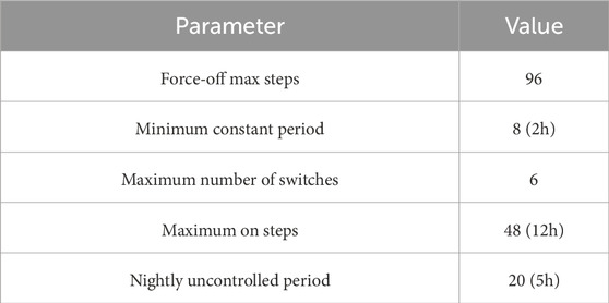
Table 1. Parameters used to generate all possible daily force-off signals.

Table 2

Table 2. Metadata used as features in the training set. Penetration scenario features describe the characteristics of the pool of simulated buildings and devices, while temporal features refer to the time of the prediction. Here, $q_{z\%}$ stands for the $z\%$ quantile.

Table 3

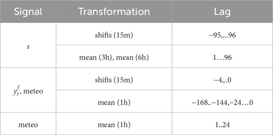
Table 3. Continuous variables, transformations, and lags passed as features to the metamodel. Meteorological information consists of temperature and global horizontal irradiance measurements.

Figure 1

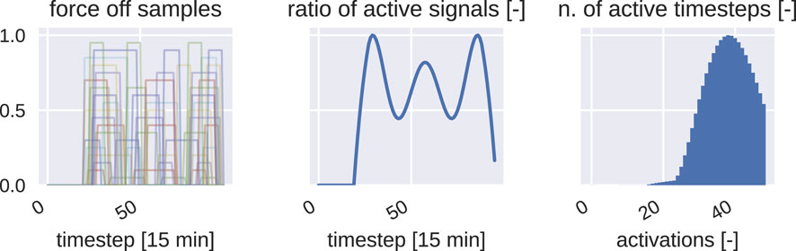
Figure 1. Left: a random sample of daily scenarios for the force-off signal. Center: ratio of active signals for a given timestep of the day. Right: distribution of the number of active timesteps among all possible scenarios.

Instead of training several metamodels using datasets with different numbers of HPs and EHs, we follow a common approach from forecasting literature and train a single global model by crafting datasets of different penetration scenarios and using them to create a single dataset. We build the final dataset following these steps:

1. We build penetration scenarios by grouping a subset of the simulated buildings, from which the aggregated power $y_t^f$ is retrieved. A dataset is then built for each penetration scenario, selecting at random $k\%$ observations from the simulated years. We sampled a total of 100 penetration scenarios and used $k=20$, for a total length of the dataset of 40 equivalent years.

2. We retrieve metadata describing the pool of buildings for each penetration scenario. Metadata include the total number of each kind of device, the mean thermal equivalent transmittance (U) of the sampled buildings, and other parameters reported in Table 2. We further augment the dataset with time features such as the hour, the day of the week, and the minute of the day of the prediction time.

3. Each penetration scenario dataset is augmented through transformations and lags of the original features, as reported in Table 3, to obtain ${\mathcal{D}}_s$.

4. The final dataset is retrieved by stacking the penetration scenario datasets $\mathcal{D}={[{\mathcal{D}}_s]}_{1:n_s}$.

To summarize, the simulation employs 15-min timesteps. Load profiles were generated using realistic consumption patterns, as explained before. Control signals were constrained to meet minimum on/off periods. Because we are targeting peak shaving, we expect that our optimization will not worsen grid stability. All simulation datasets and source data used in this study are derived primarily from publicly accessible repositories. The trained forecasting models will be made available upon publication.

3.2 Model description

The metamodel is a collection of multiple-input single-output (MISO) LightGBM regressors (LightGBM, 2024) predicting $y_t^f$ at a different step ahead. We preferred a set of non-parametric boosted models w.r.t. classic parametric ones because the first is more flexible regarding the kind of inputs. For instance, it is easy to integrate categorical variables and increase the model complexity by stacking more boosting rounds. Overfit can be controlled via the learning rate and maximum splits, increasing generalization abilities.

The alternative to a collection of MISO models is training only one MISO model after augmentation of the dataset with a categorical variable indicating the step ahead being predicted. This option was discarded due to both memory and computational time restrictions. For our dataset, this strategy requires more than 30 GB of RAM. Furthermore, training a single tree for the whole dataset requires more computational time than training a set of MISO predictors in parallel (on a dataset that is 96 times smaller). We recall that the final dataset is composed of 100 scenarios differing in the set of buildings composing the aggregated response to be predicted. This means that removing observations at random when performing a train-test split would allow the metamodel to see the same meteorological conditions present in the training set. To overcome this, the training set was formed by removing the last 20% of the yearly observations from each penetration scenario dataset ${\mathcal{D}}_s$. That is, the training-test split is done such that the training set contains only observations relative to the first 292 days of the yearly simulation.

A hyper-parameter optimization is then run on a 3-fold cross-validation over the training set; this means that each fold of the hyper-parameter optimization contains roughly 53% of $\mathcal{D}$. The tuned hyper-parameters are the learning rate and the number of estimators for the LightGBM regressors; the parameters are kept fixed for all 96 models predicting the various steps ahead. We used a fixed-budget strategy with 40 samples and used the Optuna Python package (Optuna, 2020) implementation of the tree-structured Parzen estimator (Ozaki et al., 2020) as a sequential sampler.

3.3 Ablation studies

We performed an ablation study to see the effectiveness of different sampling strategies (point (1) of the dataset-building methodology described in the previous section) and model variations.

3.3.1 Evaluation metrics

Model performances can be better compared when plotting the average (over samples and prediction times) normalized mean absolute error (nMAE) as a function of step ahead. The nMAE for the predictions generated at time $t$ is defined as:

$nMA{E}_t=\frac{{\sum }_{k=1}^{96}|y_{t+k}-{\widehat{y}}_{t+k}|}{{\sum }_{k=1}^{96}|y_{t+k}|}.(1)$

Furthermore, we define two relative energy imbalanced measures:

${\mathrm{\Delta }}_{\mathit{rel}}{E}_t=\frac{{\sum }_{k=1}^{96}{\widehat{y}}_{t+k}\left(s\right)-{\sum }_{k=1}^{96}{y}_{t+k}}{{\sum }_{k=1}^{96}{y}_{t+k}};(2)$

${\mathrm{\Delta }}_{\mathit{rel}}^{\mathit{noctrl}}{E}_t=\frac{{\sum }_{k=1}^{96}{\widehat{y}}_{t+k}\left(s\right)-{\sum }_{k=1}^{96}{\widehat{y}}_{t+k}\left(s_0\right)}{{\sum }_{k=1}^{96}{y}_{t+k}},(3)$

where $y_t$ is the simulated power, $\widehat{y}(s)$ is the power predicted by the metamodel with the control used in the simulation, and $\widehat{y}(s_0)$ is the power predicted by the metamodel using a zero force off. We can interpret ${\mathrm{\Delta }}_{\mathit{rel}}{E}_t$ as the relative error in the total energy needs w.r.t. the simulation and ${\mathrm{\Delta }}_{\mathit{rel}}^{\mathit{noctrl}}{E}_t$ as the change in the energy consumption estimated by the metamodel if the pool of flexible devices were not controlled.

3.3.2 Sampling schemes

To generate the final dataset, we tested two different sampling schemes to produce the penetration scenarios. In the first strategy, the total number of controllable devices is increased linearly, selecting randomly between households with an HP or an EH. In the second strategy, the number of the two controllable classes of devices is increased independently, co-varying the number of HPs and EHs in a Cartesian fashion, as illustrated in Figure 2.

Figure 2

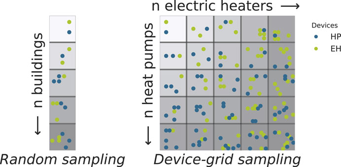
Figure 2. Sampling strategies for building the final training set. Left: the total number of controllable devices is increased linearly, selecting randomly between households with an HP or an EH. Left: the number of controllable devices is increased by independently co-varying the number of HPs and EHs.

3.3.3 Energy unbalance awareness

A physics-informed approach involving energy imbalance is proposed to enhance the accuracy of the metamodel. This method utilizes the metamodel to simulate the system’s response under two conditions: with the actual control signal $s$ and with a zeroed control signal. By subtracting these responses, we quantify the system’s “energy debt” at each timestep. This physics-based insight is crucial for improving predictions of future states. To test this hypothesis, we developed a secondary model where a set of regressors first forecasts the system response for future steps under both scenarios. The resultant energy imbalances from these predictions serve to enrich the training dataset. Subsequently, another set of regressors is trained on this augmented dataset, employing this physics-informed strategy during both training and prediction phases.

In total, we compared four distinctive configurations, comprising the two models and the two sampling strategies. Figure 3 provides representative examples of predictions of the energy-aware metamodel trained using the grid sampling strategy, featuring varying counts of controlled HPs and EHs.

Figure 3

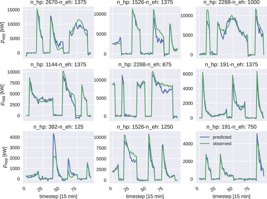
Figure 3. Random example of a day-ahead metamodel’s forecasts for different numbers of HPs and EHs, where the force off was activated at least once for the energy-aware metamodel trained using the grid sampling strategy.

The grid sampling scheme did indeed help in increasing the accuracy of the predictions w.r.t. the random sampling scheme for both the LightGBM models. Including the information about energy imbalances at each step ahead shows some benefits for both sampling strategies at the expense of a more complex model. The accuracy improvement impacts only controlled scenarios, as demonstrated by comparing the second and third panels in Figure 4. These panels show the scores obtained for instances where the force-off signal was activated at least once or never activated. This result aligns with our expectations. As an additional analysis, we studied the energy imbalance over the prediction horizon. For this analysis, we considered only the controlled cases in the test set. We removed all the instances in which the force-off signal was activated in the last 5 h of the day from the comparison. In this case, part of the consumption will be deferred outside the prediction horizon, making the comparison meaningless.

Figure 4

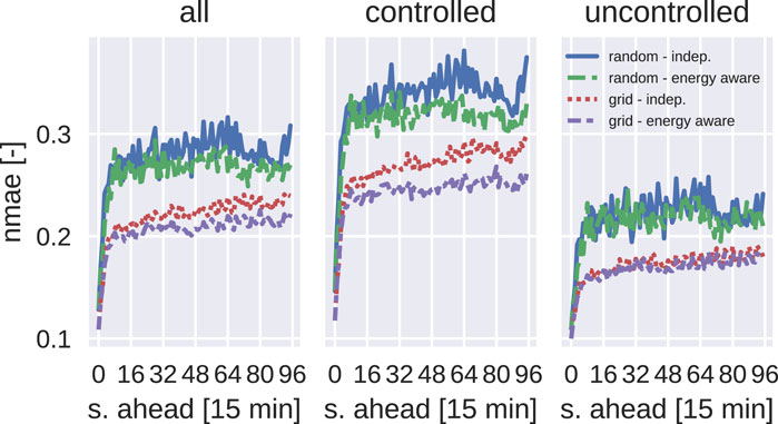
Figure 4. Performances for the four tested metamodels in terms of nMAE as a function of the step ahead.

Looking at the first row of Figure 5, we see how the empirical cumulative distribution functions (ECDFs) of ${\mathrm{\Delta }}_{\mathit{rel}}{E}_d$ and its absolute value (left and right panels) are closer to zero when the grid sampling strategy is applied. In addition, using the energy-aware model helps to make a more precise prediction in terms of used energy over the prediction horizon. For all four models, 80% of the time, the relative deviation in the horizon energy prediction lies below 20%. The second row of Figure 5 reports the change in the forecasted energy consumption within the prediction horizon with and without control. It is reasonable to think that the consumption should approximately match because the force off usually only defers the consumption. In this case, the energy-aware models present a lower difference in the consumed energy.

Figure 5

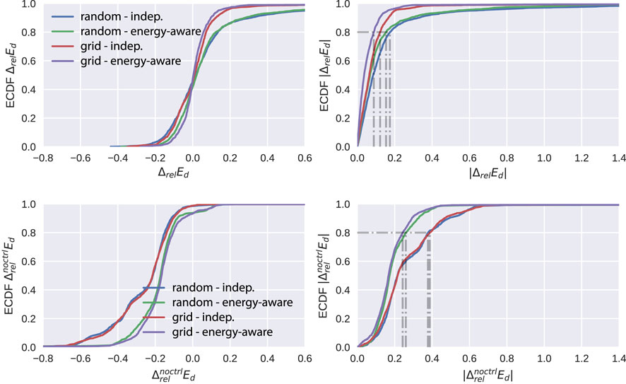
Figure 5. Left: cumulative distributions of the relative energy imbalance for different models. Right: empirical cumulative density functions of the absolute relative energy imbalance for the different models.

3.4 Characterization of the rebound effect

We used the energy imbalance aware model in combination with the grid sampling strategy to visualize rebound effects for different numbers of HPs and EHs. Figure 6 shows three extreme examples of the characterization: the penetration scenario with the maximum number of EHs and zero HPs, the converse, and the scenario where both penetrations are at their maximum value. The rebound is shown in terms of energy imbalance from the test set, such that they have a force-off signal turning off at the fifteenth plotted step. Note how different observations can start to show negative energy imbalance at different time steps; this is because force-off signals can have different lengths, as shown in Figure 1. The upper left quadrant shows the energy imbalance predicted by the metamodel in the case of the maximum number of EHs and no HPs. Comparing it with the lower right quadrant, where the sample only contains HPs, we see that the rebound effect has a quicker decay, being close to zero after only 10 steps (corresponding to 2.5 h). The lower right quadrant exhibits a markedly slower dissipation of the rebound effect, attributable to the different heating mechanisms and temporal constants inherent in systems heated by EHs and HPs. EHs, dedicated solely to DHW heating, have their activation guided by a hysteresis function governed by two temperature sensors installed at varying heights within the water tank. In contrast, HPs are responsible for both DHW and space heating, and their activation hinges on the temperature of the hydronic circuit, thus creating a segregation between the HPs and the building heating elements, namely, the serpentine. As a result, HP activation is subjected to a system possessing a heating capacity significantly greater than that of the standalone DHW tank: the building’s heating system. Further intricacy is added to the power response profile of the HP due to its dual role in catering to DHW and space heating needs, with priority assigned to the former. The visual responses presented in Figure 1 are color-differentiated according to the 7-day mean of the ambient temperature. As per the expected pattern, the EH responses exhibit independence from the average external temperature, while a modest influence can be detected for the HPs, where a rise in average temperatures aligns with a faster decay in response.

Figure 6

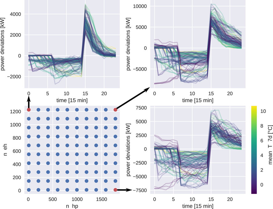
Figure 6. Example of system response in terms of deviations from the expected response (prediction where control signal features referring to feature time steps are zeroed), dependent on the number of HPs and EHs.

Our analysis reveals that while EHs tend to exhibit a slower decay in rebound effects, HPs recover more rapidly. This differential behavior has important implications for grid stability. To mitigate potential issues arising from concurrent device reactivation, we propose a dynamic grouping strategy that staggers control actions, thereby smoothing the rebound profile and enhancing overall system stability.

4 Using metamodels for optimal flexibility control

This section presents how the metamodel can be incorporated into the optimization loop, beginning with optimizing a single flexibility group. The optimization problem is formulated to minimize a composite cost function consisting of day-ahead energy costs and a peak tariff penalty. Constraints include ensuring that the force-off durations do not compromise thermal comfort and that the rebound effects remain within acceptable limits. The objective that we found most compelling from both the DSO and energy supplier perspectives is the simultaneous minimization of day-ahead costs (incurred by the energy supplier on the spot market) and peak tariff (paid by the DSO to the transmission system operator (TSO). Notably, this scenario is particularly well-suited to Switzerland, where a distinctive situation persists with the energy supplier and the DSO remaining bundled. The peak tariff, being proportionate to the maximum monthly peak over a 15-min interval, poses a more significant optimization challenge than day-ahead costs, as the peak tariff is paid on the monthly peak. Because it is extremely hard to produce accurate forecasts over a 1-month period, we solved the peak shaving problem on a daily basis as a heuristic. This then leads us to the following optimization problem:

$s^{*}=\underset{s}{\mathrm{arg\; min}}\mathcal{L}\left(\widehat{y}\left(s\right)\right);(4)$

$=\underset{s}{\mathrm{arg\; min}}\gamma \left({\displaystyle \sum _{h=1}^H}{p}_h^s{\widehat{y}}_h\left(s\right)\right)+p^p\max \left(0,\underset{h}{\max }{\widehat{y}}_h\left(s\right)-y_k^{\mathit{max}}\right),(5)$

where $h$ refers to the step ahead, $p^s\in {\mathbb{R}}^T$ is the day-ahead spot price, $p^p$ is the price for the monthly peak in $CHF/kW$, and $\gamma =dt/3600$ is a coefficient taking into account the timestep duration. The second term in Equation 5 encodes the cost of increasing the peak realized so far in the current month, $y_k^{\mathit{max}}$. Equation 4 is not trivial to solve because it is a function of a non-parametric regressor, the metamodel. However, the parameters reported in Table 1 produce a total of 155,527 control scenarios; this allows us to evaluate Equation 4 using a brute-force approach, finding the exact minimizer $s*$. This is done through the following steps:

1. Forecast the total power of the DSO: ${\widehat{y}}^{\mathit{tot}}=f_{\mathit{tot}}(x_t,{\theta }_{\mathit{tot}})$. This forecaster was obtained by training 96 different LightGBM models, one for each step ahead.

2. Forecast the baseline consumption of flexible devices, ${\widehat{y}}^f(s_0)=f(x_t,s_0,\theta )$, using the metamodel with the control signal $s=s_0$ set to zero (corresponding to not controlling the devices).

3. Forecast the response of flexible devices under a given control scenario $s$ for the next day. This is always done using the metamodel: ${\widehat{y}}^f(s)=f(x_t,s,\theta )$.

4. The objective function is evaluated on ${\widehat{y}}_t(s)={\widehat{y}}^{\mathit{tot}}-{\widehat{y}}^f(s_0)+{\widehat{y}}^f(s)$ for all the possible plausible control scenarios; the optimal control scenario $s*$ minimizing the total costs is returned.

4.1 Controlling multiple groups

As previously noted, forcing off a group of flexibilities results in a subsequent rebound effect when they are permitted to reactivate. A viable strategy to counter this issue is to segment the flexibilities into various groups, thereby circumventing a concurrent reactivation. Moreover, this segmentation method helps exploit their thermal inertia to the fullest extent. This is especially true in the context of HP, as variations in building insulation and heating system sizing inevitably lead to differences in turn-on requirements to maintain home thermal comfort under identical weather conditions. Analogous considerations apply to hot water boilers as well. In addition, it is crucial to note that, generally, EHs can endure longer force-off periods than HPs. Thus, the stratification of flexibilities into distinct groups not only mitigates the rebound effect but also facilitates the optimal utilization of the entire appliance fleet’s potential. Equation 4 can be reformulated as

$s^{*}=\underset{{\left[s_g\right]}_{g=1}^G}{\mathrm{arg\; min}}{\displaystyle \sum _{h=1}^H}{p}_h^s\left({\widehat{y}}_h^{\mathit{tot}}-{\displaystyle \sum _{g=1}^G}{\widehat{y}}_{h,g}^f\left(s_0\right)+{\displaystyle \sum _{g=1}^G}{\widehat{y}}_{h,g}^f\left(s_g\right)\right)+;(6)$

$p^p\underset{h}{\max }{\displaystyle \sum _{h=1}^H}\left({\widehat{y}}_t^{\mathit{tot}}-{\displaystyle \sum _{g=1}^G}{\widehat{y}}_{h,g}^f\left(s_0\right)+{\displaystyle \sum _{g=1}^G}{\widehat{y}}_{h,g}^f\left(s_g\right)\right),(7)$

where $G$ is the total number of groups and $s_g$ is the control signal sent to the $g_{th}$ group. Due to the combinatorial nature of the problem, a sequential heuristic is adopted, wherein control groups are optimized one after the other, thereby reducing computational complexity while maintaining near-optimal performance. The first group of devices optimizes on the uncontrolled power profile ${\widehat{y}}_t^{\mathit{tot}}$. Once the optimal control for the first group is found, the second group is optimally scheduled on $y_t^{\mathit{tot}}-{\widehat{y}}_{t,1}^f(s_0)+{\widehat{y}}_{t,1}^f(s)$, where the second subscript in ${\widehat{y}}_{t,1}$ refers to the control group. An example of such sequential optimization is shown in Figure 7, where one group of EHs and one of HPs are scheduled sequentially.

Figure 7

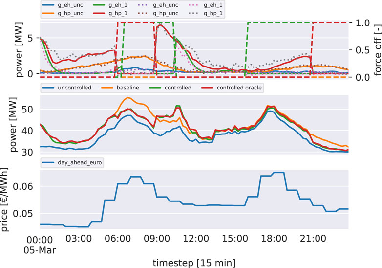
Figure 7. Example of optimized control action using the metamodel. Top: control signals (dashed), forecast group responses (dotted), and simulated, both controlled and uncontrolled, responses (thick). Middle: total power from uncontrolled DSO households (blue), total DSO power when no control action is taken (orange), and simulated and forecasted system responses (green and red). Bottom: day-ahead price on the spot market.

The upper panel shows the optimal control signals, along with the simulated response (dashed lines) and the response predicted by the metamodel (dotted lines). The middle panel shows the power from uncontrolled nodes in the DSO grid (blue), the total DSO power when no control action is taken (orange), and the simulated and forecast system response (green and red).

4.2 Ensuring comfort for the end users

To ensure end-user comfort while leveraging their flexibility, it is critical that appliances maintain the ability to meet energy demands for a certain period of time despite shorter time shifts within this duration. When a building is heated with a thermo-electric device, such as an HP, its energy consumption exhibits a significant inverse correlation with the external temperature. This correlation can be effectively illustrated using an equivalent linear resistance–capacitance (RC) circuit to model the building’s thermal dynamics. The static behavior of this model can be represented by the energy signature, which depicts the linear relationship between the building’s daily energy consumption and the mean daily external temperature, denoted as $T_d$. As more households now feature PV power plants, it becomes relevant to include the average daily global horizontal irradiance, or $I_d$, as a contributing factor in the energy signature fit. As a first approximation, we assume a linear relationship between global irradiance and PV production. Consequently, elevated $I_d$ values may correspond to lower daily energy consumption, granted a PV system is installed. However, such an effect should not be misattributed to variations in temperature. Failing to integrate $I_d$ into the regression could lead to an underestimation of the daily energy consumption when expressed as a function of temperature. The comprehensive energy signature, denoted as $e(T_d,I_d)$, emerges as a piecewise linear function reliant on the external temperature and $I_d$.

Our ultimate objective is to ascertain the necessary operational duration for a specified HP to fulfill the building’s daily energy requirements. Consequently, the total number of active hours during a day, $h$, is obtained by dividing the energy signature by the nominal power of the HP:

$h\left(T_d,I_d\right)=\frac{e\left(T_d,I_d\right)}{p_{\mathit{nom}}}.(8)$

The following steps describe our procedure to generate and control a group of HPs based on their estimated activation time:

1. Estimate the energy signatures of all the buildings with an installed HP $e_i(T_d,I_d)$.

2. Estimate the reference activation time $h_{\mathit{ref,i}}$ for worst-case conditions, that is, for $T_d=0$ and $I_d=0$.

3. At control time, perform a day-ahead estimation of activation times for all HPs, $h_i({\widehat{T}}_d,{\widehat{I}}_d)$ using a day-ahead forecast of $T_d$ and $I_d$. Use the within-group maximum values of the needed activation time, $h_{\mathit{max,g}}={\max }_{i\in \mathcal{G}}{h}_{g,i}({\widehat{T}}_d,{\widehat{I}}_d)$, to filter out control scenarios having more than $h_{\mathit{max,g}}$ force-off steps. This process guarantees that all HPs are allowed on for a sufficient time, given the temperature and irradiance conditions.

5 Using metamodels for closed-loop emulations

For testing operational and closed-loop accuracy, we simulated 1 year of optimized operations in the case in which 66% of the available flexibilities are controlled. We used two control groups: one containing only EHs, which can be forced off for a longer period of time, and one group of HPs, controlled as explained in the previous section.

The prediction error accuracy was already studied in Section 3.3, where we tested the metamodel on a simulated test set. In that case, the force-off signals in the dataset were produced by a random policy. We further tested the performance of the metamodel when predicting the optimized force-off. We could expect a difference in prediction accuracy because, in this case, the force-off signals have a non-random pattern that could influence the average error of the forecaster. In addition to this, we assessed the accuracy of the metamodel in terms of economic results in closed-loop; that is, we retrieve the errors on the economic key performance indicators (KPIs) when the simulation is completely bypassed, and the metamodel is used for both optimizing and emulating the behavior of the controlled devices.

5.1 Open-loop operational accuracy

At first, operational accuracy was assessed in terms of predictions, comparing the aggregated controlled power profile with the sum of the individually simulated (controlled) devices. Figure 8 shows the normalized daily time series of the prediction error during the actual optimization process. This is defined as

$n{ϵ}_d=\frac{y_d-{\widehat{y}}_d}{y_d},(9)$

where $y_d,{\widehat{y}}_d\in {\mathbb{R}}^{96}$ are the aggregated simulated power profiles and their day-ahead predictions, respectively. We see that we only have sporadic deviations above 10% for all the observed error paths. To have a more general understanding of the metamodel performance, in the second panel of eight, we plotted the histogram of the mean daily error, defined as $\frac{1}{96}{\sum }_{i=1}^{96}n{E}_{d,i}$. This shows that the metamodel is usually under-predicting, or over-smoothing, the true response from the simulation, which is generally the expected behavior of a forecaster trained to minimize the sum of squares loss. The fact that this distribution is contained in the −2%+2% interval, which is much narrower than in the maximum observed discrepancies in the daily error traces, confirms that high error deviations in the day-ahead predictions are only sporadic.

Figure 8

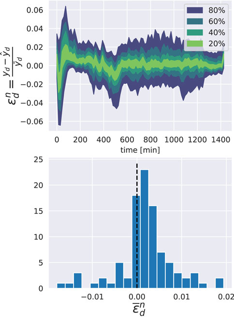
Figure 8. Performance of the metamodel in the open-loop simulations. Left: daily relative errors plotted as time series. Right: distribution of the daily means of the relative error.

5.2 Closed-loop economic performances

We cannot directly assess the closed-loop performances of the metamodel in terms of prediction errors. This is because, when simulating in a closed loop, the metamodel’s predictions are fed to itself in a recurrent fashion. This could result in slightly different starting conditions for each day; furthermore, comparing the sampled paths is not our final goal. A more significant comparison is in terms of economic returns. We compared these approaches:

1. Simulated. We run the optimization and fully simulate the system’s response. In this setting, the metamodel is only used to obtain the optimal control signal to be applied the day ahead. The controlled devices are then simulated, subject to the optimal control signal. The costs are then computed based on the simulations.

2. Forecast. For each day, the optimal predictions used for the optimization are used to estimate the cost. We simulate the controlled devices; this process is repeated the next day. This approach gives us an understanding of how the operational prediction errors shown in Figure 8 impact the estimation of the costs.

3. Emulated. The simulations are completely bypassed. The metamodel is used to optimize the control signal and generate the next-day responses for the controlled devices.

It should be clear that if the third approach gives comparable results in terms of costs, we could then simply use the metamodel for both the control task and its evaluation. This would significantly speed up the simulation loop: we will not need to simulate the thermodynamic behavior of thousands of households but only evaluate the trained metamodel, which is almost instantaneous. It could seem unlikely to reach the same accuracy produced by a detailed simulation, but this can be justified by the fact that we are only interested in an aggregated power profile, whose dimensionality is only a tiny fraction of all the simulated signals needed to produce it.

In Figure 9, we reported the relative discrepancies from economic KPIs retrieved by the simulation using the two aforementioned approaches. As an additional KPI, we also reported the estimated tons of produced $C{O}_2$. While the $C{O}_2$ emissions are not directly optimized for, minimizing the energy costs also positively impacts the emissions because energy prices correlate with the $C{O}_2$ intensity in the energy mix. The emitted $C{O}_2$ tons are estimated as

$M_{C{0}_2}={\displaystyle \sum _{t=1}^T}{C}_t{y}_t,(10)$

where $C_t$ is the carbon intensity in the national energy mix in $\frac{g_{C{O}_2}}{kWh}$. The top panel refers to the costs that would be generated considering the total power profile, $y$. In both the forecast and closed-loop cases, all costs have a deviation of less than 1%. The total cost has a deviation of well below one per thousand. In our case study, the controlled group of devices is only a small fraction of the total energy delivered by the DSO; to estimate the metamodel’s performance, it is thus important to evaluate only costs generated by controlled devices $y^f$. These are shown in the bottom panel of Figure 9, where we have normalized the objectives’ errors with the additional costs faced by the DSO due to the flexible group. In both the energy costs and the $C{O}_2$, we have a relative error below 3%, while the peak cost has a deviation of 6%. We have a comparable deviation for forecasts and closed-loop simulations. In all the cases, the peak costs are underestimated; this was to be expected, as the metamodel is trained with a sum of squares loss, which systematically underestimates extreme events. The discrepancies remain acceptable for conducting A/B testing in a simulated environment. The left panel shows discrepancies for actual costs faced by the DSO, computed using the total power profile $y$. In this case, we have roughly a ten-fold reduction in the relative error w.r.t. the simulations. This is not a surprise because, as anticipated, the controllable devices constitute only a fraction of the energy supplied by the DSO. Nevertheless, this is the quantity we are interested in. For completeness, the relative deviations and absolute costs for the simulated case relative to Figure 9 are reported in Tables 4, 5 for the total and flexible device profiles, respectively.

Figure 9

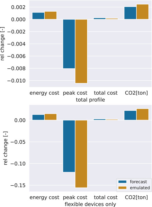
Figure 9. Deviations of different objectives from the simulated results, using the metamodel to optimize and forecast the power profiles (blue) or to completely bypass the simulation (orange). Top: relative error of objectives normalized with the total simulated costs. Bottom: relative error of objectives normalized with the additional costs faced by the DSO due to the flexible group.

Table 4

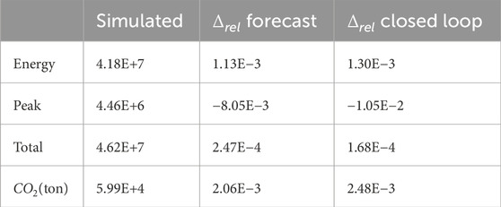
Table 4. First column: energy costs, peak, total costs, and $C{O}_2$ emissions from the controlled simulation. Second column: relative differences from the simulated costs when evaluated using the metamodel’s day-ahead predictions. Third column: relative differences from the simulated costs using the metamodel to emulate the system. Data refer to the case in which 66% of the available HPs and boilers were controlled.

Table 5

Table 5. First column: additional energy costs, peak, total costs, and $C{O}_2$ emissions faced by the DSO due to the flexibility group. The second and third columns are as in Table 4.

6 Conclusions and extensions

In this work, we presented a methodology to model the flexibility potential of controllable devices located in a DSO’s distribution grid and optimally steer it by broadcasting force-off signals to different clusters of flexible devices. We achieved this by training a non-parametric global forecasting model conditional to the control signals and the number of controlled devices to predict their simulated aggregated power. The numerical use case showed that the forecaster’s accuracy is high enough to use it as a guide to optimally steer flexible devices. Moreover, the high accuracy of economic KPIs suggests that the forecaster can be used to bypass the simulation completely and speed up A/B-like testing and the retrieval of different demand-side management policies over different device penetrations.

We envision the following possible extensions of the presented work:

$•$ Continuous control. The presented use case relied on extensive enumeration of the possible force-off signals for the day-ahead optimization. This was possible due to restrictions requested by the DSO on the shape of the control signal, which resulted in a total number of possible control signals in the order of 1E+5 scenarios. Using a higher timestep for the control will require evaluating a prohibitive number of scenarios. The approach proposed in this article can still be feasible by replacing the boosted tree with an “Optimizable” regressor, that is, either a partial input-convex neural network (Amos et al., 2017) or a conditional invertible neural network (Ardizzone et al., 2019). In this case, we can use a continuous signal $s_c\in [\mathrm{0,1}]$ indicating the fraction of flexible devices to be forced off at a given moment in time. We can then apply gradient descent to the Optimizable regressor and retrieve the optimal $s_c$.

$•$ Probabilistic forecast. The presented optimization framework is based on a deterministic formulation. Formulating the problem in the stochastic framework could be advantageous when considering peak tariffs. This would require summing two sources of uncertainty: the one associated with the prediction of the total power profile $y^{tot}$ and the one associated with the metamodel forecasts. These can be both assessed by obtaining probability distributions after the training phase through conformal prediction and using them to generate scenarios.

The methodology presented in this work offers a cost-effective and computationally efficient tool for real-time grid management, with significant implications for both the energy industry and the broader community. By enabling near-instantaneous evaluations of various demand-response scenarios, our approach facilitates the integration of renewable energy sources and enhances grid resilience. This capability not only reduces operational costs and peak tariffs for distribution system operators and energy suppliers but also contributes to lowering $C{O}_2$ emissions by optimizing flexible load management. Aggregating flexible residential loads presents clear benefits, including improved predictability of demand and reduced operational costs. However, challenges such as variability in customer behavior and differences in device characteristics must be addressed. Our approach mitigates these issues by incorporating device-specific metadata and leveraging a global forecasting framework that adapts to different aggregation scenarios. In practical terms, the forecasting model can be integrated into the operational routines of DSOs to enable day-ahead scheduling and real-time control of flexible loads. Pilot projects in regions with high renewable penetration have demonstrated similar methodologies, and our approach could be directly adapted to such environments to enhance grid efficiency and reduce energy costs. The method supports the development of more adaptive and intelligent energy systems, enabling more sustainable and resilient power grids that benefit both industry stakeholders and end users. The proposed method aligns well with emerging trends in dynamic pricing and renewable energy integration. By reducing peak tariffs and enabling more responsive demand-side management, the approach offers substantial cost savings and operational efficiencies. This not only supports current market incentives for renewable integration but also provides a pathway for future market-based grid optimization strategies. While the proposed methodology shows promising results, it is important to note that several assumptions underlie our model. These include the predictability of consumption signals and the relative homogeneity in customer behavior. Future work will focus on relaxing these assumptions by incorporating more heterogeneous data and robust control strategies to better capture real-world variability. In addition to economic benefits, our approach contributes to environmental sustainability by reducing peak load and, consequently, the reliance on fossil-fuel-based peaking power plants. The optimization of flexible load management is shown to lower overall CO₂ emissions, aligning with broader objectives of reducing the carbon footprint of the energy sector. Looking forward, emerging technologies in advanced forecasting, control, and energy storage are poised to further enhance demand-side flexibility management. These developments promise to extend the applicability of our methodology to a wider range of deferrable loads and more dynamic grid environments, ultimately driving further improvements in grid efficiency and sustainability. In practical deployments, several challenges must be addressed. First, securing active customer participation is critical, as the overall effectiveness of demand-response programs depends on sufficient enrollment and reliable customer engagement. Second, robust data security protocols are essential to protect sensitive information from unauthorized access and cyber threats. Finally, the infrastructure must be scalable and interoperable with existing systems to handle increased data flows and control signals. The proposed forecasting model is designed with modularity and compatibility in mind, which facilitates its integration into current energy management systems such as SCADA platforms and smart grid networks. Its lightweight computational requirements and adherence to industry-standard communication protocols enable seamless real-time data acquisition and control. This compatibility ensures that the model can be incorporated into both legacy systems and modernized infrastructures, thereby enhancing grid responsiveness and operational efficiency without the need for extensive overhauls.

In summary, our approach not only achieves high accuracy in predicting the aggregated response of flexible loads but also demonstrates significant potential for reducing operational costs and peak tariff expenses. The ability to bypass full-scale simulations without sacrificing economic performance paves the way for faster and more efficient grid management strategies. Moreover, our methodology provides actionable insights into the rebound effects of flexible loads, thereby supporting the design of more robust demand-response policies.

Data availability statement

The raw data supporting the conclusions of this article will be made available by the authors, without undue reservation.

Author contributions

LN: conceptualization, data curation, methodology, writing – original draft, and writing – review and editing. VM: supervision, writing – original draft, and writing – review and editing.

Funding

The author(s) declare that financial support was received for the research and/or publication of this article. This work was financially supported by the Swiss Federal Office of Energy (Optimal DSO dISpatchability (ODIS), SI/502074 and IEA Annex 82 “Energy Flexible Buildings Towards Resilient Low Carbon Energy Systems”) and the Swiss National Science Foundation under NCCR Automation (grant agreement 51NF40180545).

Conflict of interest

Author LN was a scientific advisor of Hive Power SA.

The remaining author declares that the research was conducted in the absence of any commercial or financial relationships that could be construed as a potential conflict of interest.

Generative AI statement

The author(s) declare that no Generative AI was used in the creation of this manuscript.

Publisher’s note

All claims expressed in this article are solely those of the authors and do not necessarily represent those of their affiliated organizations, or those of the publisher, the editors and the reviewers. Any product that may be evaluated in this article, or claim that may be made by its manufacturer, is not guaranteed or endorsed by the publisher.

Supplementary material

The Supplementary Material for this article can be found online at: https://www.frontiersin.org/articles/10.3389/fenrg.2025.1547617/full#supplementary-material

References

Albadi, M. H., and El-Saadany, E. F. (2007). “Demand response in electricity markets: an overview,” in 2007 IEEE power engineering society general meeting, 1–5. doi:10.1109/PES.2007.385728

CrossRef Full Text | Google Scholar

Amos, B., Xu, L., and Kolter, J. Z. (2017). “enInput convex neural networks,” in Proceedings of the 34 th international conference on machine learning. Swiss Statistical Office, 10.

Google Scholar

Ardizzone, L., Luth, C., Kruse, J., Rother, C., and Kothe, U. (2019). enGuided image generation with conditional invertible neural networks ArXiv:1907.02392 [cs]

Google Scholar

Babatunde, O. M., Munda, J. L., and Hamam, Y. (2020). Power system flexibility: a review. Energy Rep. 6, 101–106. doi:10.1016/j.egyr.2019.11.048

CrossRef Full Text | Google Scholar

Balint, A., and Kazmi, H. (2019). Determinants of energy flexibility in residential hot water systems. Energy Build. 188-189, 286–296. doi:10.1016/j.enbuild.2019.02.016016

CrossRef Full Text | Google Scholar

Biegel, B., Andersen, P., Stoustrup, J., Madsen, M. B., Hansen, L. H., and Rasmussen, L. H. (2014). Aggregation and control of flexible consumers – a real life demonstration. IFAC Proc. Vol. 47, 9950–9955. doi:10.3182/20140824-6-ZA-1003.00718

CrossRef Full Text | Google Scholar

Callaway, D. S. (2009). Tapping the energy storage potential in electric loads to deliver load following and regulation, with application to wind energy. Energy Convers. Manag. 50, 1389–1400. doi:10.1016/j.enconman.2008.12.01212.012

CrossRef Full Text | Google Scholar

Chen, K.-H. (2016). “Ripple-based control technique Part I,” in Power management Techniques for integrated circuit design (IEEE), 170–269. doi:10.1002/9781118896846.ch4

CrossRef Full Text | Google Scholar

Chen, Y., Xu, P., Gu, J., Schmidt, F., and Li, W. (2018). Measures to improve energy demand flexibility in buildings for demand response (DR): a review. Energy Build. 177, 125–139. doi:10.1016/j.enbuild.2018.08.003

CrossRef Full Text | Google Scholar

Cochran et al., J (2014). Flexibility in 21st century power systems. Available online at: https://www.nrel.gov/docs/fy14osti/61721.pdf.

Google Scholar

Corradi, O., Ochsenfeld, H., Madsen, H., and Pinson, P. (2013). Controlling electricity consumption by forecasting its response to varying prices. IEEE Trans. Power Syst. 28, 421–429. Conference Name: IEEE Transactions on Power Systems. doi:10.1109/TPWRS.2012.2197027

CrossRef Full Text | Google Scholar

Cui, W., Ding, Y., Hui, H., Lin, Z., Du, P., Song, Y., et al. (2018). Evaluation and sequential dispatch of operating reserve provided by air conditioners considering lead–lag rebound effect. IEEE Trans. Power Syst. 33, 6935–6950. Conference Name: IEEE Transactions on Power Systems. doi:10.1109/TPWRS.2018.2846270

CrossRef Full Text | Google Scholar

De Coninck, R., and Helsen, L. (2016). Quantification of flexibility in buildings by cost curves – methodology and application. Appl. Energy 162, 653–665. doi:10.1016/j.apenergy.2015.10.114apenergy.2015.10.114

CrossRef Full Text | Google Scholar

Eid, C., Codani, P., Chen, Y., Perez, Y., and Hakvoort, R. (2015). “Aggregation of demand side flexibility in a smart grid: a review for European market design,” in 2015 12th international conference on the European energy market (EEM) (ISSN), 1–5. doi:10.1109/EEM.2015.7216712

CrossRef Full Text | Google Scholar

Fischer, D., Wolf, T., Wapler, J., Hollinger, R., and Madani, H. (2017). Model-based flexibility assessment of a residential heat pump pool. Energy 118, 853–864. doi:10.1016/j.energy.2016.10.1111016/j.energy.2016.10.111

CrossRef Full Text | Google Scholar

Ghaemi, R., Abbaszadeh, M., and Bonanni, P. G. (2019). Optimal flexibility control of large-scale distributed heterogeneous loads in the power grid. IEEE Trans. Control Netw. Syst. 6, 1256–1268. Conference Name: IEEE Transactions on Control of Network Systems. doi:10.1109/tcns.2019.2933945TCNS.2019.2933945

CrossRef Full Text | Google Scholar

Jensen, S. O., Marszal-Pomianowska, A., Lollini, R., Pasut, W., Knotzer, A., Engelmann, P., et al. (2017). IEA EBC Annex 67 energy flexible buildings. Energy Build. 155, 25–34. doi:10.1016/j.enbuild.2017.08.044

CrossRef Full Text | Google Scholar

Junker, R. G., Azar, A. G., Lopes, R. A., Lindberg, K. B., Reynders, G., Relan, R., et al. (2018). Characterizing the energy flexibility of buildings and districts. Appl. Energy 225, 175–182. doi:10.1016/j.apenergy.2018.05.037

CrossRef Full Text | Google Scholar

Junker, R. G., Kallesoe, C. S., Real, J. P., Howard, B., Lopes, R. A., and Madsen, H. (2020). Stochastic nonlinear modelling and application of price-based energy flexibility. Appl. Energy 275, 115096. doi:10.1016/j.apenergy.2020.115096115096

CrossRef Full Text | Google Scholar

Kiljander, J., Gabrijelcic, D., Werner-Kytola, O., Krpic, A., Savanovic, A., Stepancic, Z., et al. (2019). Residential flexibility management: a case study in distribution networks. Ieee Access 7, 80902–80915. doi:10.1109/access.2019.2923069

CrossRef Full Text | Google Scholar

LightGBM (2024). Welcome to LightGBMs documentation! –LightGBM 3.3.1.99 documentation. Available online at: https://lightgbm.readthedocs.io/en/latest/.

Google Scholar

Mancini, F., Cimaglia, J., Basso, G. L., and Romano, S. (2021). Implementation and simulation of real load shifting scenarios based on a flexibility price market strategy–the Italian residential sector as a case study. Energies 14, 3080. doi:10.3390/en141130803390/en14113080

CrossRef Full Text | Google Scholar

Mohandes, B., Moursi, M. S. E., Hatziargyriou, N., and Khatib, S. E. (2019). A review of power system flexibility with high penetration of renewables. IEEE Trans. Power Syst. 34, 3140–3155. doi:10.1109/tpwrs.2019.28977272897727

CrossRef Full Text | Google Scholar

Muller, F., and Jansen, B. (2019). Large-scale demonstration of precise demand response provided by residential heat pumps. Appl. Energy 239, 836–845. doi:10.1016/j.apenergy.2019.01.202apenergy.2019.01.202

CrossRef Full Text | Google Scholar

Nuytten, T., Claessens, B., Paredis, K., Van Bael, J., and Six, D. (2013). Flexibility of a combined heat and power system with thermal energy storage for district heating. Appl. Energy 104, 583–591. doi:10.1016/j.apenergy.2012.11.02911.029

CrossRef Full Text | Google Scholar

Oldewurtel, F., Sturzenegger, D., Andersson, G., Morari, M., and Smith, R. S. (2013). “Towards a standardized building assessment for demand response,” in 52nd IEEE conference on decision and control (ISSN), 7083–7088. doi:10.1109/CDC.2013.6761012

CrossRef Full Text | Google Scholar

Optuna (2020). Optuna - a hyperparameter optimization framework. Available online at: https://optuna.org/.

Google Scholar

OSCP (2024). OSCP 2.0, protocols, home - open charge alliance. Available online at: https://www.openchargealliance.org/protocols/oscp-10/.

Google Scholar

Ozaki, Y., Tanigaki, Y., Watanabe, S., and Onishi, M. (2020). “Multiobjective tree-structured parzen estimator for computationally expensive optimization problems,” in Proceedings of the 2020 genetic and evolutionary computation conference (New York, NY, USA: Association for Computing Machinery), GECCO ’20), 533–541. doi:10.1145/3377930.3389817

CrossRef Full Text | Google Scholar

Palensky, P., and Dietrich, D. (2011). Demand side management: demand response, intelligent energy systems, and smart loads. IEEE Trans. Industrial Inf. 7, 381–388. doi:10.1109/TII.2011.2158841

CrossRef Full Text | Google Scholar

Parvania, M., Fotuhi-Firuzabad, M., and Shahidehpour, M. (2013). Optimal demand response aggregation in wholesale electricity markets. IEEE Trans. Smart Grid 4, 1957–1965. Conference Name: IEEE Transactions on Smart Grid. doi:10.1109/TSG.2013.2257894

CrossRef Full Text | Google Scholar

Petersen, M. K., Edlund, K., Hansen, L. H., Bendtsen, J., and Stoustrup, J. (2013). “A taxonomy for modeling flexibility and a computationally efficient algorithm for dispatch in Smart Grids,” in 2013 American control conference (ISSN), 1150–1156. doi:10.1109/ACC.2013.6579991

CrossRef Full Text | Google Scholar

Ponocko, J., and Milanovic, J. V. (2018). Forecasting demand flexibility of aggregated residential load using smart meter data. IEEE Trans. Power Syst. 33, 5446–5455. Conference Name: IEEE Transactions on Power Systems. doi:10.1109/TPWRS.2018.2799903

CrossRef Full Text | Google Scholar

Portela, C. M., Klapwijk, P., Verheijen, L., and Boer, H. d.Enexis (2015). OSCP-an open protocol for smart charging of electric vehicles

Google Scholar

Reynders, G., Diriken, J., and Saelens, D. (2017). Generic characterization method for energy flexibility: applied to structural thermal storage in residential buildings. Appl. Energy 198, 192–202. doi:10.1016/j.apenergy.2017.04.061

CrossRef Full Text | Google Scholar

Six, D., Desmedt, J., Vahnoudt, D., and Bael, J. (2011). “Exploring the flexibility potential of residential heat pumps combined with thermal energy storage for smart grids,” in 21th international conference on electricity distribution, paper, 442.

Google Scholar

Valles, M., Bello, A., Reneses, J., and Frias, P. (2018). Probabilistic characterization of electricity consumer responsiveness to economic incentives. Appl. Energy 216, 296–310. doi:10.1016/j.apenergy.2018.02.058

CrossRef Full Text | Google Scholar

Yin, L., and Qiu, Y. (2022). Long-term price guidance mechanism of flexible energy service providers based on stochastic differential methods. Energy 238, 121818. doi:10.1016/j.energy.2021.1218181016/j.energy.2021.121818

CrossRef Full Text | Google Scholar

Zheng, W., Wu, W., Zhang, B., and Lin, C. (2018). Distributed optimal residential demand response considering operational constraints of unbalanced distribution networks. Iet Generation Transm. and Distribution. doi:10.1049/iet-gtd.2017.1366

CrossRef Full Text | Google Scholar