 Amjad T. Assi
 Joshua Accola
 Gaghik Hovhannissian
 Rabi H. Mohtar
 Erik Braudeau
- 1Qatar Foundation, Qatar Environment and Energy Research Institute, Doha, Qatar
- 2Department of Agricultural and Biological Engineering, Purdue University, West Lafayette, IN, USA
- 3Department of Biological Systems Engineering, University of Wisconsin-Madison, Madison, WI, USA
- 4Institut de Recherche pour le Développement (IRD), Pédologie Hydrostructurale, Bondy, France
- 5Biological and Agricultural Engineering Department and Zachry Department of Civil Engineering, Texas A&M University, College Station, TX, USA
Accurate measurement of the two soil moisture characteristic curves, namely, water retention curve (WRC) and soil shrinkage curve (SSC) is fundamental for the physical modeling of hydrostructural processes in vadose zone. This paper is the application part following the theory presented in part I about physics of soil medium organization. Two native Aridisols in the state of Qatar named locally Rodah “räôd'ǝ” soil and Sabkha “săb'kǝ” soil were studied. The paper concluded two main results: the first one is about the importance of having continuous and simultaneous measurement of soil water content, water potential and volume change. Such measurement is imperative for accurate and consistent characterization of each of the two moisture characteristic curves, and consequently the hydrostructural properties of the soil medium. The second is about the simplicity, reliability, strength and uniqueness of identifying the characteristic parameters of the two curves. The results also confirmed the validity of the thermodynamic-based equations of the two characteristic curves presented in part I.
Introduction
The hydrostructural properties of a structured soil medium have been characterized by two fundamental curves: water retention curve (WRC) and the soil shrinkage curve (SSC). These curves have been used to evaluate the soil structure (Haines, 1923; Coughlan et al., 1991; Braudeau et al., 2004, 2005), soil physical quality (Dexter, 2004; Santos et al., 2011), soil deformation (Alaoui et al., 2011) and, in general, to characterize and model the soil-water interaction by linking the soil physical properties with their impact on the water and solute movement through a soil medium. The WRC defines the relationship between the soil-water potential and the water content, while the SSC represents the specific volume changes “or void ratio changes” of a soil due to the changes in its water content. A third fundamental characteristic curve is the unsaturated hydraulic conductivity curve. This curve is difficult to measure (Børgesen et al., 2006); hence, several scientists have used the fitted parameters of the WRC with the available pore size distribution statistical models to predict the unsaturated hydraulic conductivity curve (Burdine, 1953; Brooks and Corey, 1964; Mualem, 1976; van Genuchten, 1980).
The WRC and SSC curves have been measured in laboratory separately and by different apparatus and methods based on their end use. Generally, the measurement range (~0–900 hPa) for the WRC, which is the measurement range of the tensiometer, is suitable for soil water flow and solute transport studies. However, several techniques have been used to measure the SSC. These methods can be characterized into four groups: (i) Archimedes' principle-based approach. The well-known methods of this approach are: the resin-coated method (Brasher et al., 1966), the paraffin-coated method (Lauritzen and Stewart, 1942), and the rubber balloon method (Tariq and Durnford, 1993a). In resin-coated and paraffin-coated methods, the soil samples could be clods (Reeve and Hall, 1978), aggregates (Bronswijk, 1991), or soil cores (Crescimanno and Provenzano, 1999; Cornelis et al., 2006). While, in the rubber balloon method, reconstituted soil cores were used in most studies (Tariq and Durnford, 1993a; Cornelis et al., 2006). In this approach, the soil samples were submerged into water and then the change in the sample volume was determined from the volume of displaced fluid; (ii) physical measurement-based approach: where the soil cores “disturbed or undisturbed” dimensions were measured directly using a vernier caliper (Berndt and Coughlan, 1977; Huang et al., 2011), a linear displacement transducer (Boivin et al., 2004; Braudeau and Mohtar, 2004) or a thin metal stick (Kim et al., 1992); (iii) laser sensors-based approach: where the soil core diameter and height were determined through laser beams such as the retractometer apparatus (Braudeau et al., 1999), (iv) image-based approach: where the volume of the soil sample (either clod or core) was either scanned with a 3-D optical scanner (Sander and Gerke, 2007) or by a simple standard digital camera (Stewart et al., 2012). Several studies have discussed and compared these methods, Cornelis et al. (2006) showed that there were significant differences between the Archimedes' principle-based methods “paraffin-coated and rubber balloon methods” and the physical measurement-based methods “vernier caliper method” where the former produced more accurate and reliable data; however, Sander and Gerke (2007) observed some errors in the resin-coated method that affects the measured volume due to inadequate coating or penetration of the coating materials. Crescimanno and Provenzano (1999) highlighted the problem of anisotropy of vernier caliper method due to the use of confined cores. In general, most of these methods require a continuous measurement follow up for 2–3 weeks (Crescimanno and Provenzano, 1999; Cornelis et al., 2006) and at the end produce 10–20 data pairs.
To fulfill the modeling requirement of the water flow and solute transport through a structured soil medium, the measured discrete data set must be converted into curves by fitting the data with mathematical functions through parameters fittings. Several models were developed to fit the discrete experimental data of the WRC (e.g., El-kadi, 1985; Leij et al., 1997; Groenevelt and Grant, 2004; Fredlund et al., 2011). These WRC models consider the soil as a rigid porous medium whose porosity is represented by equivalent bundle of capillary tubes (Braudeau and Mohtar, 2004; Coppola et al., 2012), their state variables are referenced to a virtual volume, Representative Elementary Volume (REV), which ignores the soil structure (Braudeau and Mohtar, 2009), and their parameters usually have no physical meaning (Chertkov, 2004). However, other researchers (Voronin, 1980; Berezin et al., 1983) followed a thermodynamic-based approach for defining the relationships between the soil water potential and water content by using physiochemical parameters and variables. Several models were developed to define the known shrinkage phases (Figure 1) of the SSC termed structural, normal, basic and residual by identifying the inflection point of the assumed S-shape of the curve (McGarry and Malafant, 1987; Peng and Horn, 2005), transition points between the shrinkage phases which were named as: shrinkage limit point, air entry point, the macropore shrinkage limit point, and the maximum swelling point (e.g., Giráldez et al., 1983; McGarry and Daniells, 1987; McGarry and Malafant, 1987; Kim et al., 1992; Tariq and Durnford, 1993b; Braudeau et al., 1999), the curvature at the transition zones between the shrinkage phases (e.g., Olsen and Hauge, 1998; Peng and Horn, 2005), the slopes of the tangents of the transition points (Peng and Horn, 2005), and the slope of saturation line (Giráldez et al., 1983). Still, other studies (Groenevelt and Grant, 2002; Chertkov, 2003) used empirical coefficients and parameters to model the SSC. Few scientists have tried to integrate these shrinkage characteristic points and/or slopes in modeling the water and solute transport through structured soil medium (Armstrong et al., 2000; Larsbo and Jarvis, 2005; Coppola et al., 2012). However, these models still reference their state variables to virtual volume of soil medium (REV). Moreover, the SSC could be differentiated by the presence or lack of some shrinkage phases. Peng and Horn (2013) identified six types of SSCs based on the number of the existing shrinkage phases in the shrinkage curves by using a large set of experimental data. Finally, few scientists tried to integrate the shrinkage curve.
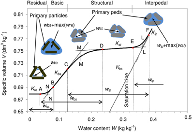
Figure 1. Various configurations of air and water partitioning into the two pore systems, inter and intra primary peds, related to the shrinkage phases of a standard Shrinkage Curve [water content vs. specific volume]. The various water pools [wre, wbs, wst, and wip] are represented with their domain of variations. The linear and curvilinear shrinkage phases are delimited by the transition points (A–F). Points N′, M′, and L′ are the intersection points of the tangents at those linear phases of the Shrinkage Curve. (Adapted from Braudeau et al., 2004).
Compared with the existing studies, this study presents three new issues regarding to: the type of the studied soil; the apparatus used for measuring the WRC and SSC, and the models used for both WRC and SSC. Two native Aridsols, according to US soil taxonomy, in the State of Qatar were investigated in this study. This class of soil has rarely been considered in the shrinkage behavior studies. Then, a new apparatus (Bellier and Braudeau, 2013) was used to continuously and simultaneously measure the data pairs for WRC (gravimetric water content vs. soil suction/potential) and SSC (gravimetric water content vs. specific volume) for eight unconfined soil cores and through a complete drying cycle. Frequent and continuous measurements (approximately every 10 min for 2–3 days under a constant temperature of 40°C) provide essential visual presentations of the two continuous curves (i.e., WRC and SSC) including the shape, the inflection points, and the shrinkage phases which are vital for modeling the curves as discussed before. Such a continuous capture and portrayal of the discrete data can't be obtained by other methods, mainly in the case of the SSC. Also, simultaneous measurements, of the same soil core, ensure having the data pairs for WRC and SSC, which are usually measured separately, under similar conditions (same temperature, humidity, etc.) and same water contents which are considered as the main state variable in all soil water models. None of the existing methods except (Boivin et al., 2004; Braudeau and Mohtar, 2004) give such a measurement. Some studies showed that the different drying rates of the same soil sample affect the WRC behavior (Zhou et al., 2014) and the soil shrinkage and cracking behavior (Tang et al., 2010). These findings strengthen the need for having continuous and simultaneous measurements under consistent conditions which simulates reality. The use of unconfined soil cores decrease the anisotropic shrinkage behavior highlighted by Crescimanno and Provenzano (1999). In addition, the number of the sampled cores (8 samples each time) and the automated measurements reduce the time and effort needed to carry out such measurements. Finally, new models for WRC and SSC were used in this study. These models were developed based on the Pedostructure and SREV concept (Braudeau and Mohtar, 2009) and the Gibbs thermodynamic potential function of the soil medium (Sposito, 1981) and recently presented in Part 1 of this study (Braudeau et al., 2014).
Thus, the objectives of this study were to: (1) introduce a new characterization approach of a soil medium based on continuous measurements of soil water potential and soil shrinkage, (2) establish a methodology for preparing reconstituted and undisturbed soil samples for apparatus' measurements, (3) evaluate the efficiency of this kind of characterization where each parameter has a physical meaning and quantifies a specific hydrostructural property of the Pedostructure. Two native Aridsoils in the State of Qatar were investigated in this study.
Materials and Methods
The WRC and SSC Thermodynamic Equations
In Part 1 of this study, Braudeau et al. (2014) were able to derive the following state functions of the pedostructure:
The equation of the pedostructure WRC:
where, W is the pedostructure water content excluding the saturated interpedal water [kgwater kg−1soil], Wma gravimetric macropore water content “outside the primary peds” [kgwater kg−1soil], Wmi gravimetric micropore water content “inside the primary peds” [kgwater kg−1soil], Ema is potential energy of surface charges positioned on the outer surface of the clay plasma of the primary peds [Jkg−1solid], Emi is potential energy of surface charges positioned inside the clay plasma of the primary peds [Jkg−1solid], hmi is the soil suction inside the primary peds [dm ~ kPa], hma is the soil suction outside the primary peds [dm ~ kPa], ρw is the specific density of water [1kgwater dm−3].
The equations of the pedostructure micro and macro pore water contents at equilibrium were derived such that:
and
where, A is a constant, such that: , E = Emi + Ema and WmiSat and WmaSat are the micro and macro water content at saturation such that WSat = WmiSat + WmaSat.
Finally, the SSC of the pedostructure was derived such that:
where, Kbs, Kst, and Kip are the slopes at inflection points of the measured shrinkage curve at the basic, structural, and interpedal linear shrinkage phases, respectively [dm3 kg−1water], and wbs, wst, and wip are the water pools associated to the linear shrinkage phases of the pedostructure in [kgwater kg−1soil] (Figure 1); V is the specific volume of the pedostructure [dm3 kg−1soil], and V0 is the specific volume of the pedostructure at the end of the residual phase [dm3 kg−1soil].
The values of the water pools associated with the basic shrinkage phase (wbs), the structural shrinkage phase (wst), and the interpedal shrinkage phase (wip) can be determined as shown in the following relationships:
where, kN and kL represent the vertical distance between the intersection points N-N′, and L-L′ (Figure 1) on the shrinkage curve [kgsoil kg−1water], WeqmiN is the micro-pore water content calculated by [Equation (2b)] but by using WN instead of W, WN is the water content at the intersection point (N′) in Figure 1 and represents the water content of the primary peds at dry state such that WN = max(wre) [kgwater kg−1soil], wre is the water pool associated with the residual shrinkage phase of the shrinkage curve [kgwater kg−1soil], WL is the water content at the intersection point (L′) (Figure 1) such that WL = WM + max(wst) [kgwater kg−1soil], and WM is the water content at the intersection point (M′) (Figure 1) such that WM = WN + max(wbs) and it represents the saturated water content of the micropore domain [kgwater kg−1soil].
Anyhow, different soil types have different structures and hence different shapes of the SSC. Peng and Horn (2013) identified six types of shrinkage curves based on the number of shrinkage phases observed in the measured shrinkage curve. The data set used in their study was discrete measurement consisting of 10–30 data pairs. However, as shown in Part 1, Braudeau et al. (2014) identified three main types of the shrinkage curves based on: the shape of the curve (Sigmoidal or not), and the existence of the saturated interpedal water which is responsible for the shrinkage phase parallel to the saturation line (i.e. slope = 1). They used continuous measurements of 200–600 data pairs. The three identified types were: (i) Sigmoidal shrinkage curve without saturated interpedal water, (ii) Sigmoidal shrinkage curve with saturated interpedal water, and (iii) Non-sigmoidal shrinkage curve. However, we are interested in types (i) and (iii) as they represent the shapes of the shrinkage curves of the studied soil.
To summarize, the state variables and the physical parameters describing a structured soil medium can now be characterized in three thermodynamically-based characteristic functions: (1) the micro and macro pedostructure water contents functions [Weqmi(W) and Weqma(W)], (2) the water retention function [h(W)], and (3) the soil shrinkage function [V(W)]. However, the question is now how to identify the physical parameters of these functions, this question will be answered in details later in the paper, but let's first recall that in total, there are 12 hydrostructural parameters: V0, WN, kN, Kbs, Kst, Emi, Ema, WmiSat, WmaSat, WL, kL, Kip where four of them are common parameters for the three characteristic functions (Emi, Ema, WmiSat, and WmaSat) and three of them (WL, kL, Kip) are only used in the shrinkage curve of sigmoidal shape with saturated interpedal water. This shape of curves wasn't among the shrinkage curves obtained for the studied soil. Thus, in this study, only 9 hydrostructural parameters were used for characterizing the soil medium organization “pedostructure.” These are the parameters of the three characteristic functions, such that:
- The pedostructure micro and macropore water content curves [Weqmi(W) and Weqma(W)]: EA, Ema/A, “i.e., Emi, Ema, WmiSat, and WmaSat.”
- The water retention curve [h(W)]: Emi, Ema, WmiSat, and WmaSat.
- The soil shrinkage function [V(W)]: V0, WN, kN, Kbs, Kst, Emi/A, Ema/A, WmiSat, WmaSat.
Finally, the continuous and simultaneous measurements provided a strong and reliable visualization of the transition points and slopes of the different shrinkage phases of the shrinkage curves. Such visualization was very imperative for extracting and estimating the hydrostructural parameters as it is discussed later in this paper.
Soils Studied
Two native soils, classified as Aridisols in US Soil Taxonomy, located near Al Khor city in the State of Qatar were used in this study (see Table 1). These native soils are: (1) Rodah soil: “Rodah” is an Arabic word means a garden and it is locally used for the colluvium depressions soils which have been accumulated with recent colluvial materials (mainly calcareous loamy and silty deposits) by the storm water runoff through wadis “ephemeral streams.” This soil is potentially the most suitable soil for agricultural uses, and hence most of the farms in the State of Qatar are located over these depressions, (2) Sabkha soil: “Sabkha” is also an Arabic word used for the highly saline depression soils “i.e., salt marshes.” The salts accumulation is due to the evaporation of the saline groundwater coming from the sea. In this study, the two native soils were taken from two depressions (Rodah and Sabkha) that are about 1 Km apart from each other (see Table 1), both depressions are located over a Haplocalcids great group according to US soil taxonomy (Soil Survey Staff, 1975) where limestone is the dominant outcropping formation (Scheibert et al., 2005). Finally, the Rodah and Sabkha soils used in this study have silty clay loam texture and silty loam texture, respectively.
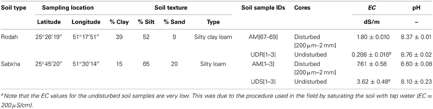
Table 1. General description of the soil samples used in the study.
Sampling and Samples Preparation
Disturbed and undisturbed soil cores were considered in this study for each soil type. The soil samples were taken from the top layer (usually 0–10 cm depth) for both types of cores. The procedures for both types of soil core preparation are explained in the following sub-sections.
Disturbed soil samples
In this study, soils were collected from the field then air-dried and then sieved using 200 μm and 2 mm sieves. This range of particle sizes (200 μm–2 mm) was selected in this study to get soil cores with macro-aggregates and hence with good structures, and also to minimize the presence of loose fine sand and silt particles and crystallized salts especially in the case of Sabkha soil. After that, the soil aggregates were filled in thin layers (Figure 2A) in a Polyvinyl chloride (PVC) rings (Φ = 5 cm, h = 5 cm) whose internal walls were coated with a thin petroleum jelly film to prevent the soil adhering to the wall during construction and to make the removal of the soil cores easier after construction. Note that unconfined soil cores were used in the analyses. During the filling process, the PVC cores were placed in small pans partially filled with water (about 5 mm deep). Whatman filters No. 40 were used to hold the soil aggregates inside the PV cores. The soil aggregates were added in thin layers (about 1 cm) with gentle tapping at the edge of the PVC ring after adding each layer. The second soil layer had not to be added until the first layer saturated to maintain well-constructed cores without horizontal segmentation. Once the cores construction was finished, a gentle leveling of the soil surface was performed. Then, the soil cores were taken and placed in an oven set at 40°C for approximately 48 h. This process allowed the soil aggregates to shrink until the end of the basic shrinkage phase and enhanced producing a structured soil medium. The time for drying could vary based on the soil type and soil salinity. After that, the soil cores were re-saturated by replacing them in the saturating pans and allowing the cores to saturate. Then, they were dried for a second time by placing them in an oven set at 40°C for about 48 h. This was the procedure for preparing a well-constructed soil aggregates cores.
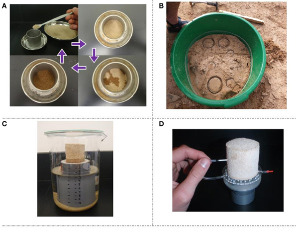
Figure 2. Steps for preparing the soil samples for TypoSoil™ analyses: (A) preparing disturbed soil sample, (B) taking undisturbed soil samples from the field, (C) saturating the unconfined soil samples by capillary through placing them on a near saturated sand box bath (−2 cm of water), (D) placing the soil sample on the perforated supporting platform and inserting the porous ceramic cup mini Tensiometer in the middle of the unconfined core.
Undisturbed soil samples
Undisturbed soil samples were also taken from both Rodah and Sabkha soils for better understanding and comparison purposes. After selecting the sampling points, the top soil layer (about 7 cm thick) was saturated by using Infiltrometer. Then, the same PVC rings (Φ = 5 cm, h = 5 cm) were used to take the soil samples (see Figure 2B). The saturation process was done to eliminate the swelling effect on the soil structure of these confined cores once they were re-saturated in the lab. The soil cores were then removed, labeled, and covered with two caps.
Preparing the soil samples for TypoSoil™ measurements
The soil cores (disturbed and undisturbed) were then saturated by capillary wetting by placing them on a sand box bath (the water level in the bath is 2 cm below the top of the sand box). As shown in Figure 2C, the sand box is simply a (Φ = 7.6 cm, h = 12 cm) PVC tube placed in a bath (2000 ml beaker). The saturation process lasted for (1–2 days) and operated under atmospheric pressure (Dickson et al., 1991; Braudeau et al., 1999; Salahat et al., 2012) and with a looking glass on top of the beaker to minimize the evaporation. The PVC rings were removed after a short time. The porous ceramic cup mini Tensiometer and the support platform which contains the pressure gauge were prepared for hosting the soil cores. Both the tensiometer and support platform must be free from any air bubbles. This process was done by flushing the system with degassed, deionized water to minimize the effects of the osmotic potentials in measurement. Then, the tensiometers were inserted (Figure 2D).
The Apparatus: TypoSoil™ [Soil Typology]
The new apparatus (Bellier and Braudeau, 2013), TypoSoil™, is a device intended to measure continuously and simultaneously the two soil moisture characteristic curves: WRC and SSC for eight (100 cm3) unconfined cylindrical soil cores. The continuous measurement of the two characteristic curves enables the user to identify precisely the characteristic points and/or portions of the curves that are used to predict the soil moisture characteristic functions. The simultaneous measurements guarantee that the soil moisture characteristic curves are measured under identical condition which is not the case in the existing devices.
The WRC is a relationship between soil suction/potential and gravimetric water content, while the SSC is a relationship between the specific volume (volume/mass of solids) and the gravimetric water content. Hence, both curves are related to the gravimetric water content. This point was taken into account while making the measurements in this device. The whole set of measurements (soil weight, dimensions, and suction) are recorded instantaneously when the soil core weight is taken.
TypoSoil™ is a modified device of the retractometer (Braudeau et al., 1999). The later measures only the SSC while the new device measures both SSC and WRC. The new device consists of the following components (Figure 3): (i) A biological stove working on a fixed temperature identified by the user (usually 30–40°C). (ii) An electronic analytical balance with MonoBloc weighting cell with a connection point's plate fixed on it. This plate closes the electrical circuit to measure and record the data once contacted with the support platform as explained below (see also Figure 3). (iii) Laser sensors: one spot laser sensor that measures the height of the soil sample by triangulation (10 μm resolution) and two thru-beam sensors (5 μm resolution) to measure the diameter of the soil sample by measuring the portion of the beam not intercepted by the laser, (iv) turning plate which can house 8 cylindrical soil samples (100 cm3 “Φ = 5 cm, h = 5 cm”) placed on perforated support platform which contains a pressure gauge inside connected to the soil core by a ceramic-needle tensiometer with an approximate functional range of 0–700 hPa. This rotating plate automatically descends to make a contact between the bottom of the perforated support platform and the connection points fixed on the balance to take and record the measurements (soil weight, dimensions, and suction). The turning plate ascends and rotates to make the measurement for another soil sample. In general, a full cycle of measurements for the 8 cores can be done in 10 min and can be repeated until the sample's weight remains constant (usually it takes 2–3 days at 40°C). Then the sample is oven dried at 105°C to determine its weight Ms (structural mass or mass of solids), (v) control panel with screen for displaying the data during and after the experiment, power and emergency stop bottoms, USB, SD Card, and Ethernet connections to download the data.
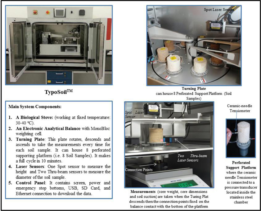
Figure 3. TypoSoil™ with its main components and how they function to measure continuously and simultaneously the soil weight (by a balance), soil suction (by a porous ceramic cup mini tensiometer), and the soil dimensions (by one spot laser sensor to measure the height and two thru-beam laser sensors to measure the diameter).
Assuming an isotropic radial shrinkage and uniform distribution of the soil water content throughout the unconfined cylindrical soil cores, the specific volume and the soil water content of the soil core can be identified, respectively, such that:
where, V is the specific volume of the soil sample [dm3 Kg−1solid], D and H are, respectively, the measured diameter and height of the soil sample [dm], Ms is the dry mass of the soil sample at 105°C [kgsolid].
where, W is the specific water content of the soil sample [Kgwater kg−1solid], m is the measured mass of the soil sample [kgwater], Ms is the dry mass of the soil sample at 105°C [kgsolid].
The saturation line [VSat] was calculated by using the following equation (Braudeau et al., 2005):
where, W is the specific water content of the soil sample [Kgwater kg−1solid], ρw is the specific density of water [1kgwater dm−3], Vs is the specific volume of the soil phase, estimated from the particle density, [dm3 Kg−1solid].
Extraction and Estimation of Pedostructure Characteristic Parameters [Hydro-Structural Parameters]
The proper modeling of water flow and solute transport through a structured soil medium requires continuous characteristic curves (WRC and SSC) instead of discrete experimental data. In this section, the procedures used for extracting and estimating the hydro-structural parameters of the proposed equations for the pedostructure WRC [h(W)], SSC [V(W)], and the micro and macro water contents at equilibrium [Weqmi(W) and Weqma(W)] from the continuously and simultaneously measured data pairs were discussed. In total, there are twelve parameters: WmiSat, WmaSat, Emi, Ema, V0, WN, kN, Kbs, Kst, WL, kL, Kip. However, the last three parameters (WL, kL, Kip) were not included in this study as they are related to the existence of interpedal water shrinkage phase which was not the case for the types of soil used in this study. Table 2 provides a comprehensive summary about these parameters, their units and the how they were estimated. The parameters extraction and estimation procedure included the following steps: (i) identify the type of the shrinkage curve, (ii) extract and/or give initial estimates of the values of WRC parameters, (WmiSat, WmaSat, Emi, Ema) (Figures 4, 5; Table 2), (iii) minimize the sum of square errors between modeled and measured WRC by using the Microsoft Excel solver, (iv) extract and/or give initial estimates of the values of SSC parameters (WmiSat, E/Ema, V0, WN, kN, Kbs, Kst) (Figures 4, 5; Table 2), and (v) minimize the sum of square errors between modeled and measured SSC by using the Microsoft Excel solver.
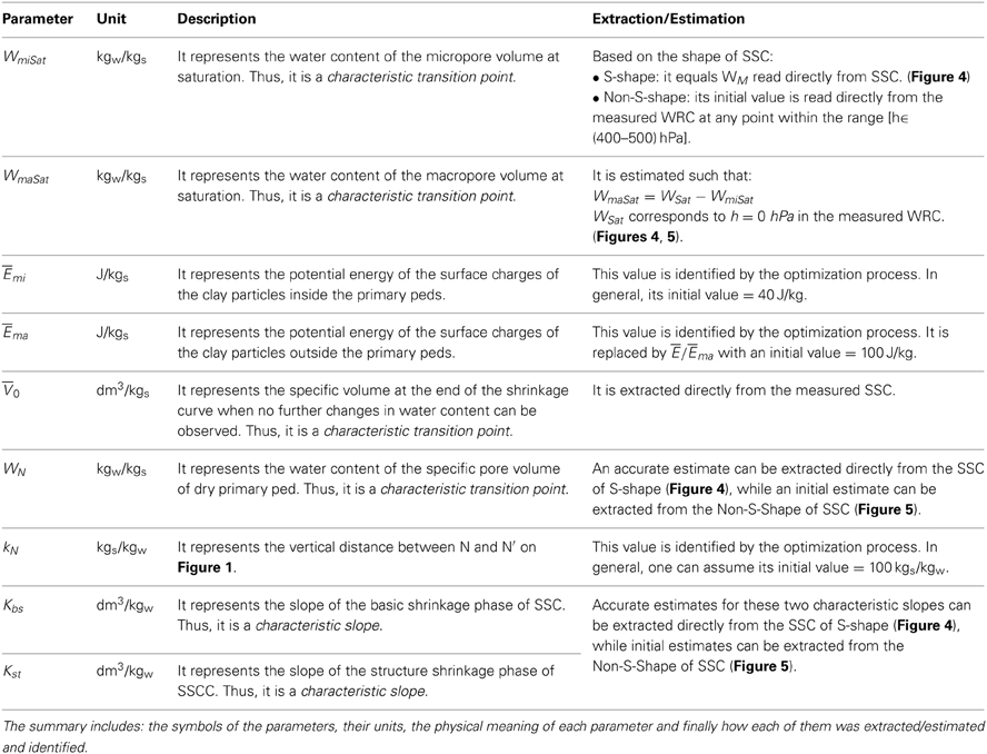
Table 2. A summary for all the characteristic parameters, included in this study, for both WRC and SSC.
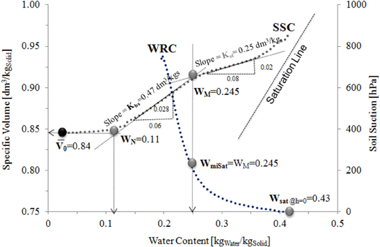
Figure 4. Extracting the characteristic parameters of WRC and SSC in the case of sigmoidal shrinkage curve with no saturated interpedal water [Core#AM69]. The black dot and text indicate that the parameters are fixed to the extracted values, while the gray dots and texts indicate that these parameters could be changed during the optimization.
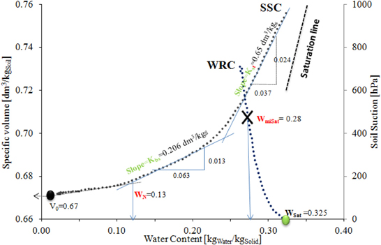
Figure 5. Extracting the characteristic parameters in the case of non-sigmoidal shrinkage curve [Core # UDR2]. The black dot and text indicate that the parameters are fixed to the extracted values, the gray dots and texts indicate that these parameters were optimized by using the MS Excel solver, while the X indicates rough estimate for the parameters.
The first step in the parameters extraction and estimation process was identifying the shape of the SSC. This step is fundamental because it affects the procedures for the parameters extraction and estimation. In this study, two types were identified: sigmoidal shape without saturated interpedal segment and Non-sigmoidal shapes.
The case of sigmoidal shrinkage curve without saturated interpedal segment
In the case of sigmoidal shrinkage curve without saturated interpedal segment, the different shrinkage phases (residual, basic, and structural) and the transition points among these phases (N and M) could easily be recognized on the measured SSC. This precise distinguishing was only possible due to having continuous measurements of the data pairs (water content and specific volume) of SSC. The following steps were followed for identifying the hydrostructural parameters of the WRC and the SSC:
Extracting and estimating the parameters of WRC. According to Equation (1), the parameters of WRC are: WmiSat, WmaSat, Emi, and Ema. The first two parameters (WmiSat, WmaSat)represent the water contents of the micropore and macropore volume at saturation, respectively. They were extracted directly from the measured WRC and SSC (Figure 4), such that:WmiSat = WM, and WmaSat = WSat − WmiSat. However, the other parameters Emi, Ema represent the potential energy of the surface charges of the clay particles inside and outside the primary peds, respectively. These parameters were given initial values, such that: Emi = 40 J/kg and Ema was replaced by E/Ema with initial value = 100 J/kg. Finally, the sum of square errors, between the modeled [using the extracted/estimated parameters in Equation (1)] and the measured WRC, was minimized by using the Microsoft Excel solver.
Extracting and estimating the parameters of SSC. According to Equations (3–6), the parameters of SSC are: (WmiSat, E/Ema, V0, WN, kN, Kbs, Kst). The first two parameters have already been identified from the previous step knowing that E = Emi + Ema. Then, V0 and Kbs which represent respectively the specific volume at the end of the shrinkage curve and the slope of the basic shrinkage phase were extracted precisely from the measured shrinkage curve (Figure 4), these two values were assumed fixed and weren't included in the optimization process. However, WN and Kst which represent respectively the water content of the specific pore volume of dry primary peds and the slope of the structural shrinkage phase were estimated as shown in Figure 4, then they were included in the optimization process. Finally, kN was given in initial value of 100 kgs/kgw. Thus, only three parameters (WN, Kst, and kN) were optimized in the process of minimizing the sum of square errors, between the modeled [using the extracted/estimated parameters in Equations (3–6)] and the measured SSC, by using the Microsoft Excel solver.
The case of non-sigmoidal shrinkage curve
In the second case, the non-sigmoidal shape of the SSC, one could not identify any mark on the measured shrinkage curve for the positions of the transition points (N, M, and L). However, thanks to the continuous measured data points, the three shrinkage phases of the shrinkage curve (residual, basic, and structural) could be distinguished on the measured curve and hence the slope parameters Kbs, Kst could be measured directly from the available data (Figure 5).
Extracting and estimating the parameters of WRC. Similar procedures for extracting and estimating the hydrostructural parameters of the WRC in the first were followed in this case, but with one exception. The initial value of WmiSat was located on the measured WRC between the potential range 400–500 hPa (Figure 5). This step was done because it was very difficult to identify the transition point (M) between the basic and the structural phases on the shrinkage curve in such a case. At the end, the four parameters (WmiSat, WmaSat, Emi, Ema) were included in the optimization process.
Extracting and estimating the parameters of SSC. Similar to the first case, but WN was roughly estimated on the shrinkage curve (the “X” in Figure 5), and Kbs, Kst were measured from the data as shown in the same figure. Finally, the parameters (WN, Kst, kN, and Kbs) were included in the optimization process. However, Kbs was included this time in the optimization process to minimize the effect of the curve's shape.
Results
The Measured Water Retention and Soil Shrinkage Curves
The continuous and simultaneous measurements of the WRCs and SSCs for reconstituted and undisturbed Rodah soil samples are shown in Figure 6, while Figure 7 shows the measurements for the reconstituted and undisturbed Sabkha soil samples. Three replicates of disturbed, constructed from aggregates of size range (200 μm–2 mm), and undisturbed soil samples for both soil types: Rodah and Sabkha Soils were analyzed by the TypoSoil™. The measured SSCs for reconstituted soil samples (Figures 6A, 7A) showed high departure from the Saturation Line. Such a departure could be a side-effect of such a macro-aggregate soil medium (200 μm–2 mm). During the construction and preparation procedures, the samples were saturated from bottom with (2 cm suction sand box). This could produce some voids filled with air and thus lack complete saturation. However, this was not the case in the undisturbed soil samples (Figures 6B, 7B). Still, the interpedal shrinkage phase parallel to the load line was absent in all samples. Regarding the shrinkage behavior of the soil samples “i.e., the range of the specific volume changes from saturation until dry state,” Rodah soil samples showed higher shrinkage amplitude values compared to the Sabkha soil samples. The specific volume changes for reconstituted Rodah soil samples ranged between “0.85 and 0.95” (i.e., the range = 0.1) dm3/kgs, undisturbed Rodah soil samples “0.68–0.75” (i.e., the range = 0.07) dm3/kgs. Reconstituted Sabkha soil samples ranged “0.85–0.88” (i.e., the range = 0.03) dm3/kgs, and the undisturbed Sabkha soil samples “0.76–0.8” (i.e., the range = 0.04) dm3/kgs. Two reasons could be considered for explaining the higher shrinkage amplitude of Rodah soil compared with the Sabkha soil; (1) the soil texture for Rodah soil is (silty clay loam) while the Sabkha soil is (silty loam), thus Rodah soil has higher clay content and lower sand content and consequently higher shrinkage amplitude; (2) the higher salinity of Sabkha soil compared with Rodah Soil (Table 2) affects the amount of water lost through evaporation during the drying cycle (2–3 days) and reduced the shrinkage of the sample. However, extending the time of drying cycle in the case of Sabkha was meaningless as the samples showed an increase in their specific volumes as shown in Figure 7. Moreover, the undisturbed soil samples showed steeper WRCs for both soil types compared with the reconstituted soil sample; this was a result of the selected aggregate size.
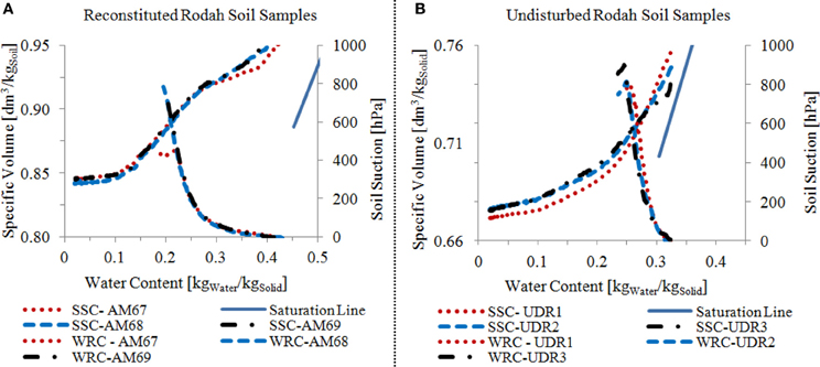
Figure 6. The measured soil moisture characteristic curves for Rodah soil: Water Retention Curve [WRC] and Soil Shrinkage Curve [SSC] for (A) the three replicates of reconstituted Rodah soil samples (aggregate size: 200 μm–2 mm); (B) the three replicates of undisturbed Rodah soil samples.
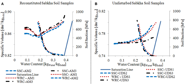
Figure 7. The measured soil moisture characteristic curves for Sabkha soil: Water Retention Curve [WRC] and Soil Shrinkage Curve [SSC] for (A) the three replicates of reconstituted Sabkha soil samples (aggregate size: 200 μm–2 mm); (B) the three replicates of undisturbed Sabkha soil samples.
The reconstituted Rodah soil samples [AM67, AM68, and AM69] had almost an S-shape for the SSCs (Figure 6A) with steep slopes of the basic shrinkage phases of the shrinkage curves. S-shape usually indicates a good soil structure (Braudeau et al., 1999; Boivin et al., 2004; Peng and Horn, 2005, 2013) and these samples were constructed from macro-aggregates (200 μm–2 mm) excluding all the fine sand and loose silt particles less than 200 μm. Figure 6A shows a very good match of the measured WRC and SSC for the three replicates. This good match indicates that samples preparing procedures were reliable. Small variation was observed at the beginning (saturation state) and at the end of the shrinkage curve (dry state), such variations could be due to: (1) different saturated initial states for different samples; (2) different initial volumes of the samples (~ 100 cm3). Finally, as shown in Figure 6A, the measured soil potential for sample (AM67) was only up to 400 hPa.
The reconstituted Sabkha soil samples [AM1, AM2, and AM3] had similar shrinkage and WRCs, but there was a shift in both curves of sample AM2. However, the shrinkage curves of the three samples showed dramatic increase in their specific volumes after a certain point (Figure 7A) which had the same water content in the three replicates (this water content ≈ 0.17 kgwater/kgsoil). Moreover, it was also noticed that this water content was almost the same water content where the tensiometer readings reached the air entry point of the tensiometers (Figure 7A). Actually, such a behavior was reported by Boivin et al. (2006), they interpreted this increase in specific volume as a result of breaking the water meniscus between sand particles due to the drying. However, this particular behavior wasn't observed in reconstituted Rodah soil samples [AM67, AM68, and AM69] which were prepared by similar procedures. Thus, the soil preparation methodology couldn't be blamed for such a behavior. However, the only determinable difference between these samples is the soil salinity. The soil salinity of the reconstituted Rodah soil samples was 1.80 ± 0.01 mS/cm, while it was 7.61 ± 0.58 for the reconstituted Rodah soil samples. The soil salinity was measured for the soil samples after being analyzed by TypoSoil™ and by using a multi-parameter meter with soil solution of (1:5 soil/water ratio). Salinity affects the soil flocculation by enhancing the bending of fine particles together (Abu Sharar et al., 1987), side by side with the aggregate size and the drying of the soil samples could lead to disjoining the aggregates and increasing gradually the sample volume. Nevertheless, this part of the shrinkage curve was excluded in the analysis.
The shapes of the SSCs for the undisturbed soil samples for both Rodah (Figure 6B) and Sabkha (Figure 7B) soils were non-sigmoidal. Moreover, those soil samples had lower saturated water content compared with the reconstituted soil samples as those samples were more compacted compared to the reconstituted ones. Two samples of the undisturbed Rodah [UDR2 and UDR3] showed similar WRC and SSC, while the third one [UDR1] had slightly shifted curves as shown in Figure 6B. In the SSC, three shrinkage phases could, somehow, be distinguished. They are: residual, basic, and structural shrinkage phases. This distinction was more difficult in the case of the undisturbed Sabkha soil samples [UDS1, UDS2, and UDS3] as shown in Figure 7B. The samples for both undisturbed Rodah and Sabkha soils showed a steep slope for the structural shrinkage phase of the SSC which indicated a high impact of the removal of the structural macropore water on the shrinkage behavior of such types of soil. Soil sample UDS3 was an exception; it didn't show the same behavior nor showed a similar shrinkage curve.
Modeling the Water Retention and Soil Shrinkage Curves
In this section, two processes were evaluated: (1) the extraction and estimation of the hydrostructural parameters from the continuous and simultaneous data pairs of the two characteristic curves (WRC and SSC); and (2) the efficiency of the thermodynamic and pedostructure based equations to model the two soil moisture characteristic curves (WRC and SSC) using such kind of hydrostructural parameters. In total, there are 12 hydrostructural parameters, while in this study only nine of them were used (V0, WN, kN, Kbs, Kst, Emi, Ema, WmiSat, WmaSat) due to the obtained shapes of the measured SSC. Nine parameters are still a large number and can be considered as a disadvantage compared to the other existing models. However, the following points should be kept in mind once doing such a comparison: (i) each parameter has a physical meaning and quantifies a specific hydrostructural property of the soil medium; (ii) six parameters (V0, WN, Kbs, Kst, WmiSat, WmaSat) out of nine can be extracted from well identified locations (points and slopes) on the measured SSC and WRC (see Figures 4, 5) and the accuracy of such a process depends on having continuous and simultaneous measurements, such measurements can be provided by TypoSoil™, and it also depends on the shape of curve as shown in section Extraction and Estimation of Pedostructure Characteristic Parameters [Hydro-structural Parameters]; thus (iii) it ends up having only three parameters (kN, Emi, Ema) to be optimized and used for modeling both soil moisture characteristic curves (SSC and WRC).
As discussed before in section Extraction and Estimation of Pedostructure Characteristic Parameters [Hydro-structural Parameters], two types of SSCs were observed in this study: sigmoidal without interpedal shrinkage phase and non-sigmoidal shrinkage curves. The procedures for extracting and estimation the hydrostructural parameters were clearly discussed in that section. Comparing the initially extracted parameters from the measured curves with the ones obtained after the optimization process, the Sigmoidal curves were much better than the other type. As shown in Figure 4, the extracted parameters of a sigmoidal shrinkage curve sample [AM69] were such that: WmiSat = 0.245, WmaSat = 0.185, WN = 0.11, Kbs = 0.47, Kst = 0.25, and V0 = 0.84. The obtained results from the optimization process were (Table 3): WmiSat = 0.24, WmaSat = 0.19, WN = 0.10, Kbs = 0.46, Kst = 0.28, and V0 = 0.84. Such a perfect matching ensured the accuracy of the extraction procedures for those physical parameters and the importance of having continuous and simultaneous measurements of the two characteristic curves. On the contrary, the characteristic points and segments that identify the hydrostructural parameters were not easily identified in the non-sigmoidal shrinkage curve. Still some good pairing was observed between the extracted parameters from the measured curves and the optimized ones Figure 5 presents an example of this type of curves for sample [UDR2], the extracted parameters from the measured curves were: WmiSat = 0.28, WmaSat = 0.045, WN = 0.13, Kbs = 0.206, Kst = 0.26, and V0 = 0.673; while, the optimized ones were: WmiSat = 0.28, WmaSat = 0.05, WN = 0.17, Kbs = 0.37, Kst = 0.62, and V0 = 0.67. Here, the only parameters that showed variation between the two sets of parameters were WN and Kbs which represent the inflection point between the basic and residual shrinkage phases and the slope of the basic shrinkage curves, respectively. Such a variation was expected due to the difficulty of identifying these characteristic points and segments on such a type of shrinkage curves. These results highlighted three imperative conclusions. The first is that the extraction methodology of the hydrostructural parameters is adequate. The second is the imperative nature of having continuous and simultaneous measurements of the two characteristic curves. The third is the simplicity of the method in identifying multiple parameters, six parameters out of nine, (V0, WN, Kbs, Kst, WmiSat, WmaSat) for two fundamental characteristic curves of the soil medium in one step.
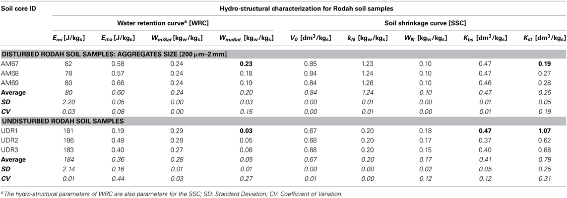
Table 3. Hydro-structural parameters for the water retention curves and soil shrinkage curves of the reconstituted and undisturbed Rodah soil samples.
Examples for the modeled WRCs and SSCs by using the extracted/optimized parameters are shown in Figures 8, 9. The results were very promising as shown in the curves of the reconstituted Rodah soil sample [AM68] (Figure 8A), undisturbed Rodah soil sample [UDR3] (Figure 8B), reconstituted Sabkha soil sample [AM1] (Figure 9A), and the undisturbed Sabkha soil sample [UDS2] (Figure 9B). A statistical summary of the excellent matching between the measured characteristic curves and modeled ones for all soil samples is shown in Table 5. In the case of WRC, 99.80–99.99% of the variation in the measured data could be explained by the modeled ones with root mean square errors (RMSEs) ranging between (2.2 and 4.5) hPa. While, for the SSC, 98.4–99.98% of the variation in the measured data could be explained by the modeled ones with RMSEs ranging between (9.3 × 10⁻⁴ − 1.5 × 10⁻²) dm3/kgsolid. It should be kept in mind that the measurement and modeled WRC curves were for the range of the readings of the tensiometers. This excellent matching between the measured characteristic curves and modeled ones supports the validity, adequacy and reliability of the extraction methodology of the hydrostructural parameters and the thermodynamic-based equations of the two characteristic curves.
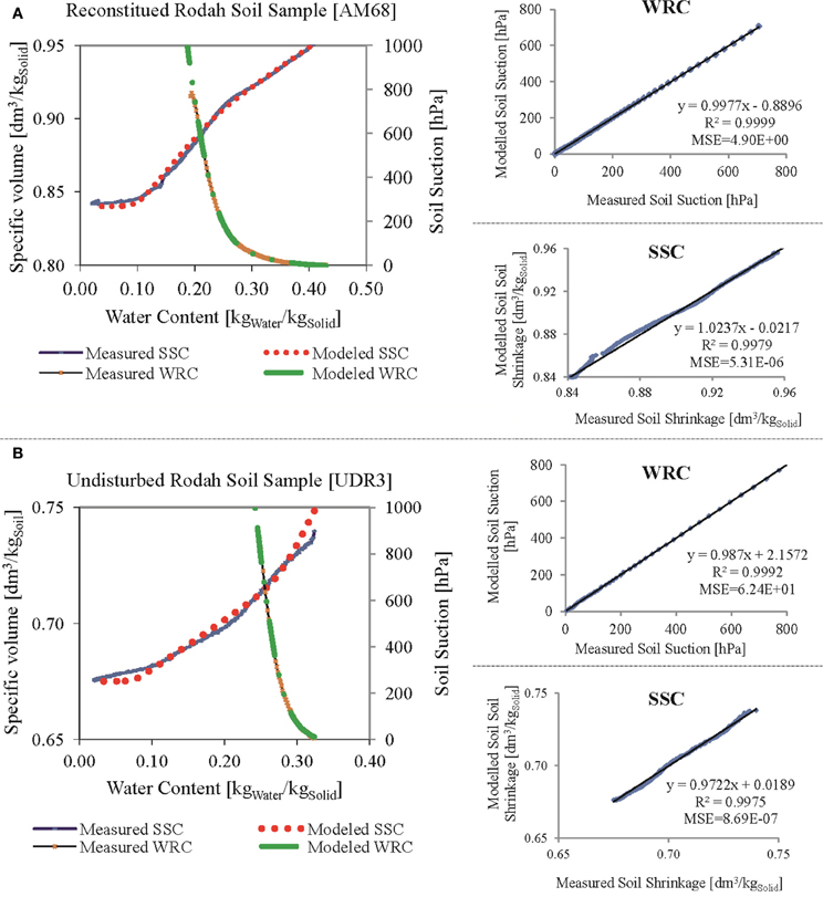
Figure 8. Examples of modeling the soil moisture characteristic curves for Rodah soil. (A) Reconstituted sample [AM68]; (B) Undisturbed sample [UDR3]. WRC, Water Retention Curve; SSC, Soil Shrinkage Curve; R2, coefficient of determination; MSE, Mean Square Errors.
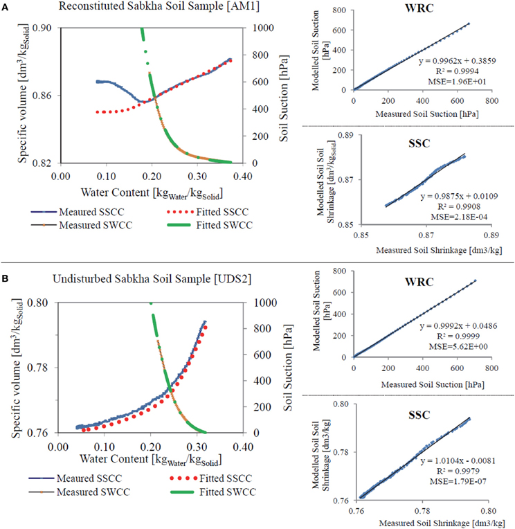
Figure 9. Examples of modeling the soil moisture characteristic curves for Sabkha soil. (A) Reconstituted sample [AM1]; (B) Undisturbed sample [UDS2]. WRC, Water Retention Curve; SSC, Soil Shrinkage Curve; R2, coefficient of determination; MSE, Mean Square Errors.
Finally, the issue of uniqueness of these hydrostructural parameters for a specific soil type was evaluated. “Uniqueness” is whether the three replicates produced the same hydrostructural parameters and whether these parameters are different from other soil types. A statistical summary of the hydrostructural parameters for Rodah soil samples and Sabkha soil samples are shown in Tables 3, 4, respectively. This summary provided sufficient evidence to support the uniqueness of the hydrostructural parameters for each soil type, these evidences were: (i) the parameters (Emi, WmiSat, V0, kN, and WN) were almost the same for three replicates in each group, see the values of standard deviations (SD) and coefficient of variation (CV), (ii) the observed variations in the parameters (WmaSat, Kbs, Kst) are justifiable. It was obvious from the measured curves (Figures 6, 7) that there was one sample of each group that had different soil shrinkage or retention curves, these samples were: (a) sample [AM67] in the reconstituted Rodah soil group showed a different shape of the structural shrinkage phase, which was characterized by Kst and highly affect Wma as shown in Equations (3) and (5). Ignoring these two parameters Kst and WmaSat of this sample (highlighted bold in Table 3), the other two replicates have similar values, such that: Kst = 0.27 and 0.29, and WmaSat = 0.18 and 0.19, respectively for the samples [AM68] and [AM69]. Moreover, the values of Kbs for all samples were the same, Kbs = 0.47, 0.47 and 0.46, respectively, for the samples [AM67, 68, 69]; (b) sample [UDR1] in the undisturbed Rodah soil group showed a different shape and a shift of the structural and basic shrinkage phases (Figure 6B), these phases were characterized by Kst and Kbs and highly affected Wma. Ignoring these three parameters Kst, Kbs and WmaSat of this sample (highlighted bold in Table 3), the other two replicates provided similar values, such that: Kst = 0.62 and 0.68, Kbs = 0.37 and 0.40 and WmaSat = 0.05 and 0.06, respectively for the samples [UDR2] and [UDR3]; (c) In the case of reconstituted Sabkha soil, sample [AM3] had a different shape of the structural shrinkage phase and thus slightly affected the parameters Kst and WmaSat; and (d) In the case of undisturbed Sabkha soil, it was obvious from Figure 7B, that the shape of the SSC of soil sample [UDS3] was totally different than the others, this was reflected mainly in the two characteristic parameters of the slopes of shrinkage phases Kst and Kbs. Ignoring this sample, the other two replicates provided similar values, such that: Kst = 0.30 and 0.35; Kbs = 0.06 and 0.05, respectively, for the samples [UDS1] and [UDS2]. Finally, (e) the parameter Ema showed some variations among the three replicates, but it was noticed that the highest variations were for the same samples that had problems as identified before (i.e., UDR1, AM3, and UDS3). Two points could be concluded from these results. There is power in the physical meaning of the used parameters in justifying and explaining any observed variations in the measured characteristic curves (WRC and SSC), and the identified hydrostructural parameters were unique for each soil sample group.
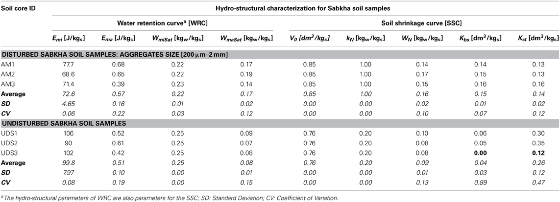
Table 4. Hydro-structural parameters for the water retention curves and soil shrinkage curves of the reconstituted and undisturbed Sabkha soil samples.
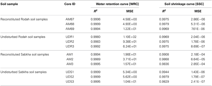
Table 5. Statistical summary of the comparison between the measured and modeled water retention curves and soil shrinkage curves of the Rodah and Sabkha soil samples.
Discussion
This paper presents a comprehensive work for measuring, characterizing, and modeling the soil shrinkage and WRCs based on the thermodynamic and Pedostructure concepts. It includes: (1) a methodology for preparing disturbed and undisturbed soil samples to be ready for the analyses by the new device, TypoSoil™. This device provides simultaneous and continuous measurements for the data pairs required to construct the two curves; (2) presentation of a simple and reliable method for extracting and estimating the hydrostructural parameters for the two curves; and (3) an application of the proposed work of Braudeau et al. (2014), in a hyper-arid region soil including very salty soil, for modeling the WRC and SSC according to the thermodynamic theory of the Pedostructure. To conduct this study, two native Aridisols in the state of Qatar, named locally “Rodah soil” and “Sabkha soil” were used. Three replicates of reconstituted and undisturbed soil cores were prepared and studied in this paper.
The results of the measured curves by the new device proved that the procedure for preparing the samples is reliable and reproducible. Minor variations were observed among the WRC and SSC of the three replicates of each soil type, except one case (UDS3). Moreover, the paper highlighted the importance of having continuous and simultaneous measurements for this kind of characterization where each parameter not only quantifies a specific physical property of the soil medium but also, in most cases, extracted from specific characteristic points and segments on the measured SSC, such as: (V0, WN, kN, Kbs, Kst), or identified at once from the two curves, such as: (WmiSat, WmaSat).
The paper portrays the simplicity, robustness, uniqueness, and accuracy of the method used for extraction of the 9 hydrostructural parameters. Very accurate values of multiple parameters (6 out of 9 parameters!) were extracted at once and in a simple way from the measured curves. These parameters were: (V0, WN, Kbs, Kst, WmiSat, WmaSat). In general, the extracted parameters for the sigmoidal shrinkage curves were more accurate than the case of non-sigmoidal shrinkage curves. This is due to the difficulty of identifying the characteristic points on the shrinkage curve. Moreover, the results evidenced the uniqueness of these parameters for each soil type.
Finally, excellent matching was observed between the measured characteristic curves and modeled ones based the thermodynamic theory of the Pedostructure. There is enough supporting evidence for the validity, adequacy and reliability of the extraction methodology of the hydrostructural parameters and the thermodynamic-based equations of the two characteristic curves. Moreover, the final values of the hydrostructural parameters proved the uniqueness of these parameters for each soil type.
These promising results open the doors for further studies, such as: using the power and uniqueness of these parameters for other studies related to the water flow and solute transports and soil remediation.
Conflict of Interest Statement
The authors declare that the research was conducted in the absence of any commercial or financial relationships that could be construed as a potential conflict of interest.
Acknowledgments
Input from the following people from Valorhiz SAS company is highly acknowledged: Hassan Boukcim and Estelle Hedri.
References
Abu Sharar, T. M., Bingham, F. T., and Rhoades, J. D. (1987). Stability of soil aggregates as affected by electrolyte concentration and composition. Soil Sci. Soc. Am. J. 51, 309–314. doi: 10.2136/sssaj1987.03615995005100020009x
Alaoui, A., Lipiec, J., and Gerke, H. H. (2011). A review of the changes in the soil pore system due to soil deformation: a hydrodynamic perspective. Soil Till. Res. 115–116, 1–15. doi: 10.1016/j.still.2011.06.002
Armstrong, A. C., Matthewes, A. M., Portwood, A. M., Leeds-Harrison, P. B., and Jarvis, N. J. (2000). CRACK-NP: a pesticide leaching model for cracking clay soils. Agric. Water Manag. 44, 183–199. doi: 10.1016/S0378-3774(99)00091-8
Bellier, G., and Braudeau, E. (2013). Device for Measurement Coupled with Water Parameters of Soil. Geneva: WO 2013/004927 A1, World Intellectual Property Organization, European Patent Office.
Berezin, P. N., Voronin, A. D., and Shein, Y. V. (1983). An energetic approach to the quantitative evaluation of soil structure. Pochvovedeniye 10, 63–69.
Berndt, R. D., and Coughlan, K. I. (1977). The nature of changes in bulk density with water content in a cracking clay. Aust. J. Soil Res. 15, 27–37. doi: 10.1071/SR9770027
Boivin, P., Garnier, P., and Tessier, D. (2004). Relationship between clay content, clay type, and shrinkage properties of soil samples. Soil Sci. Soc. Am. J. 68, 1145–1153. doi: 10.2136/sssaj2004.1145
Boivin, P., Garnier, P., and Vauclin, M. (2006). Modeling the shrinkage and water retention curves with the same equations. Soil Sci. Soc. Am. J. 70, 1082–1093. doi: 10.2136/sssaj2005.0218
Børgesen, C., Jacobsen, O., Hansen, H., and Schaap, M. (2006). Soil hydraulic properties near saturation, an improved conductivity model. J. Hydrol. 324, 40–50. doi: 10.1016/j.jhydrol.2005.09.014
Brasher, B. R., Franzmeier, D. P., Valassis, V., and Davidson, S. E. (1966). Use of saran resin to coat natural soil clods for bulk density and water retention measurements. Soil Sci. 101:108. doi: 10.1097/00010694-196602000-00006
Braudeau, E., Assi, A. T., Boukcim, H., and Mohtar, R. H. (2014). Physics of the soil medium organization part 1: thermodynamic formulation of the pedostructure water retention and shrinkage curves. Front. Environ. Sci. 2:4. doi: 10.3389/fenvs.2014.00004
Braudeau, E., Costantini, J. M., Bellier, G., and Colleuille, H. (1999). New device and method for soil shrinkage curve measurement and characterization. Soil Sci. Soc. Am. J. 63, 525–535. doi: 10.2136/sssaj1999.03615995006300030015x
Braudeau, E., Frangi, J. P., and Mothar, R. H. (2004). Characterizing non-rigid dual porosity structured soil medium using its shrinkage curve. Soil Sci. Soc. Am. J. 68, 359–370. doi: 10.2136/sssaj2004.0359
Braudeau, E., and Mohtar, R. H. (2004). Water potential in non-rigid unsaturated soil-water medium. Water Resour. Res. 40, 1–14. doi: 10.1029/2004WR003119
Braudeau, E., and Mohtar, R. H. (2009). Modeling the soil system: bridging the gap between pedology and soil-water physics. Glob. Planet. Change J. 67, 51–61. doi: 10.1016/j.gloplacha.2008.12.002
Braudeau, E., Sene, M., and Mohtar, R. H. (2005). Hydrostructural characteristics of two African tropical soils. Eur. J. Soil Sci. 56, 375–388. doi: 10.1111/j.1365-2389.2004.00679.x
Bronswijk, J. J. B. (1991). Relationship between vertical soil movements and water content changes in cracking clays. Soil Sci. Soc. Am. J. 55, 1120–1226. doi: 10.2136/sssaj1991.03615995005500050004x
Brooks, R. H., and Corey, A. T. (1964). Hydraulic Properties of Porous Media. Hydrology Paper No. 3. Fort collins, CO: Colorado State University.
Burdine, N. T. (1953). Relative permeability calculations from pore-size distribution data. J. Petrol. Technol. 5, 71–78. doi: 10.2118/225-G
Chertkov, V. Y. (2003). Modelling the shrinkage curve of soil clay pastes. Geoderma 112, 71–95. doi: 10.1016/S0016-7061(02)00297-5
Chertkov, V. Y. (2004). A physically based model for the water retention curve of clay pasts. J. Hydrol. 286, 203–226. doi: 10.1016/j.jhydrol.2003.09.019
Coppola, A., Gerke, H., Comegna, A., Basile, A., and Comegna, V. (2012). Dual-permeability model for flow in shrinking soil with dominant horizontal deformation. Water Resour. Res. 48:W08527. doi: 10.1029/2011WR011376
Cornelis, W. M., Corluy, J., Medina, H., Díaz, J., Hartmann, R., Van Meirvenne, M., et al. (2006). Measuring and modelling the soil shrinkage characteristic curve. Geoderma 137, 179–191. doi: 10.1016/j.geoderma.2006.08.022
Coughlan, K. J., McGarry, D., Loch, R. J., Bridge, B., and Smith, D. (1991). The measurement of soil structure. Aust. J. Soil Res. 29, 869–889. doi: 10.1071/SR9910869
Crescimanno, G., and Provenzano, G. (1999). Soil shrinkage characteristic curve in clay soils: measurement and prediction. Soil Sci. So. Am. J. 63, 25–32. doi: 10.2136/sssaj1999.03615995006300010005x
Dexter, A. R. (2004). Soil physical quality: part II. Friability, tillage, tilth and hard-setting. Geoderma 120, 215–225. doi: 10.1016/j.geoderma.2003.09.005
Dickson, E. L., Rasiah, V., and Groenvelt, P. H. (1991). Comparison of four pre-wetting techniques in wet aggregate stability determination. Can. J. Soil Sci. 7, 67–72. doi: 10.4141/cjss91-006
El-kadi, A. I. (1985). On estimating the hydraulic properties of soil, part 1. Comparison between forms to estimate the soil- water characteristic function. Adv. Water Resour. 8, 136–147. doi: 10.1016/0309-1708(85)90054-5
Fredlund, D. G., Sheng, D., and Zhao, J. (2011). Estimation of soil suction from the soil-water characteristic curve. Can. Geotech. J. 48, 186–198. doi: 10.1139/T10-060
Giráldez, J. V., Sposito, G., and Delgado, C. (1983). A general soil volume change equation: I. The two-parameter model. Soil Sci. Soc. Am. J. 47, 419–422. doi: 10.2136/sssaj1983.03615995004700030005x
Groenevelt, P. H., and Grant, C. D. (2002). Curvature of shrinkage lines in relation to the consistency and structure of a Norwegian clay soil. Geoderma 106, 235–245. doi: 10.1016/S0016-7061(01)00126-4
Groenevelt, P. H., and Grant, C. D. (2004). A new model for the soil-water retention curves that solves the problem of residual water content. Eur. J. Soil Sci. 55, 479–485. doi: 10.1111/j.1365-2389.2004.00617.x
Haines, W. B. (1923). The volume changes associated with variations of water content in soil. J. Agric. Sci. Camb. 13, 296–311. doi: 10.1017/S0021859600003580
Huang, C., Shao, M., and Tan, W. (2011). Soil shrinkage and hydrostructural characteristics of three swelling soils in Shaanxi, China. J. Soils Sediments 11, 474–481. doi: 10.1007/s11368-011-0333-8
Kim, D. J., Vereecken, H., Feyen, J., Boels, D., and Bronswijk, J. J. B. (1992). On the characterization of properties of an unripe marine clay soil: I. Shrinkage processes of an unripe marine clay soil in relation to physical ripening. Soil Sci. 153, 471–481. doi: 10.1097/00010694-199206000-00006
Larsbo, M., and Jarvis, N. J. (2005). Simulating solute transport in a structured field soil: uncertainty in parameter identification and predictions. J. Environ. Qual. 34, 621–634. doi: 10.2134/jeq2005.0621
Lauritzen, C. W., and Stewart, A. J. (1942). Soil-volume changes and accompanying moisture and pore-space relationships. Soil Sci. Soc. Am. Proc. 6, 113–116. doi: 10.2136/sssaj1942.036159950006000C0019x
Leij, F., Russell, W., and Lesch, S. M. (1997). Closed-form expressions for water retention and conductivity data. Ground Water 35, 848–858. doi: 10.1111/j.1745-6584.1997.tb00153.x
McGarry, D., and Daniells, I. G. (1987). Shrinkage curve indices to quantify cultivation effects on soil structure of a Vertisol. Soil Sci. Soc. Am. J. 51, 1575–1580. doi: 10.2136/sssaj1987.03615995005100060031x
McGarry, D., and Malafant, K. W. J. (1987). The analysis of volume change in unconfined units of soil. Soil Sci. Soc. Am. J. 51, 290–297. doi: 10.2136/sssaj1987.03615995005100020005x
Mualem, Y. (1976). A new model for predicting the hydraulic conductivity of unsaturated porous media. Water Resour. Res. 12, 513–522. doi: 10.1029/WR012i003p00513
Olsen, P. A., and Hauge, L. E. (1998). A new model of the shrinkage characteristic applied to some Norwegian soils. Geoderma 83, 67–81. doi: 10.1016/S0016-7061(97)00145-6
Peng, X., and Horn, R. (2005). Modeling soil shrinkage curve across a wide range of soil types. Soil Sci. Soc. Am. J. 77, 372–372. doi: 10.2136/sssaj2004.0146
Peng, X., and Horn, R. (2013). Identifying six types of soil shrinkage curves from a large set of experimental data. Soil Sci. Soc. Am. J. 69, 584–592. doi: 10.2136/sssaj2011.0422
Reeve, M. J., and Hall, D. G. M. (1978). Shrinkage in clayey sub-soils of contrasting structure. J. Soil Sci. 29, 315–323. doi: 10.1111/j.1365-2389.1978.tb00779.x
Salahat, M., Mohtar, R. H., Braudeau, E., Schulze, D., and Assi, A. (2012). Toward delineating hydro-functional soil mapping units using the pedostructure concept: a case study. Comput. Electron. Agric. 86, 15–25. doi: 10.1016/j.compag.2012.04.011
Sander, T., and Gerke, H. H. (2007). Noncontact shrinkage curve determination for soil clods and aggregates by three-dimensional optical scanning. Soil Sci. Soc. Am. J. 71, 1448–1454. doi: 10.2136/sssaj2006.0372
Santos, G. G., Silva, E. M., Marchaõ, R. L., Silveira, P. M., Braund, A., James, F., et al. (2011). Analysis of physical quality of soil using the water retention curve: validity of the S-index. C. R. Geosci. 343, 295–301. doi: 10.1016/j.crte.2011.02.001
Scheibert, C., Stietiya, M., Sommer, J., Schramm, H., and Memah, M. (2005). The Atlas of Soils for the State of Qatar, Soil Classification and Land Use Specification Project for the State of Qatar, Ministry of Municipal Affairs and Agriculture, General Directorate of Agricultural Research and Development, Department of Agricultural and Water Research. Doha: Ministry of Municipal Affairs and Agriculture.
Soil Survey Staff. (1975). Soil Taxonomy: A Basic System Soil Classification for Making and Interpreting Soil Surveys. USDA-SCS Agriculture Handbook 436. Washington, DC: U.S. Government Printing Office.
Stewart, R. D., Abou Najm, M. R., Rupp, D. E., and Selker, J. S. (2012). An image-based method for determining bulk density and the soil shrinkage curve. Soil Sci. Soc. Am. J. 76, 1217–1221. doi: 10.2136/sssaj2011.0276n
Tang, C., Cui, Y., Tang, A., and Shi, B. (2010). Experiment evidence on the temperature dependence of desiccation cracking behavior of clayey soils. Eng. Geol. 114, 261–266. doi: 10.1016/j.enggeo.2010.05.003
Tariq, A. R., and Durnford, D. S. (1993a). Soil volumetric shrinkage measurements: a simple method. Soil Sci. 155, 325–330. doi: 10.1097/00010694-199305000-00003
Tariq, A. R., and Durnford, D. S. (1993b). Analytical volume change model for swelling clay soils. Soil Sci. Soc. Am. J. 57, 1183–1187. doi: 10.2136/sssaj1993.03615995005700050003x
van Genuchten, M. Th. (1980). A closed-form equation for predicting the hydraulic conductivity of unsaturated soils. Soil Sci. Soc. Am. J. 44, 892–898. doi: 10.2136/sssaj1980.03615995004400050002x
Voronin, A. D. (1980). The structure-energy conception of the hydro-physical properties of soils and its practical applications. Pochvovedeniye 12, 35–46.
Keywords: soils in hyper-arid regions, Rodah soil, Sabkha soil, soil shrinkage curve (SSC), water retention curve (WRC), hydrostructural parameters, pedostructure and SREV concept
Citation: Assi AT, Accola J, Hovhannissian G, Mohtar RH and Braudeau E (2014) Physics of the soil medium organization part 2: pedostructure characterization through measurement and modeling of the soil moisture characteristic curves. Front. Environ. Sci. 2:5. doi: 10.3389/fenvs.2014.00005
Received: 29 January 2014; Accepted: 11 March 2014;
Published online: 31 March 2014.
Edited by:
Christophe Darnault, Clemson University, USAReviewed by:
Nabeel Khan Niazi, University of Agriculture Faisalabad, PakistanWieslaw Fialkiewicz, Wroclaw University of Environmental and Life Sciences, Poland
Copyright © 2014 Assi, Accola, Hovhannissian, Mohtar and Braudeau. This is an open-access article distributed under the terms of the Creative Commons Attribution License (CC BY). The use, distribution or reproduction in other forums is permitted, provided the original author(s) or licensor are credited and that the original publication in this journal is cited, in accordance with accepted academic practice. No use, distribution or reproduction is permitted which does not comply with these terms.
*Correspondence: Rabi H. Mohtar and Erik Braudeau, Biological and Agricultural Engineering Department and Zachry Department of Civil Engineering, Texas A&M University, 302 B Scoates Hall, Mail Stop 2117, College Station, TX 77843-2117, USA e-mail:ZXJpay5icmF1ZGVhdUBpcmQuZnI=;bW9odGFyQHRhbXUuZWR1