Climate analogs for agricultural impact projection and adaptation—a reliability test

Bos, Swen P. M.; Pagella, Tim; Kindt, Roeland; Russell, Aaron J. M.; Luedeling, Eike

doi:10.3389/fenvs.2015.00065

ORIGINAL RESEARCH article

Front. Environ. Sci., 06 October 2015

Sec. Agroecology

Volume 3 - 2015 | https://doi.org/10.3389/fenvs.2015.00065

Climate analogs for agricultural impact projection and adaptation—a reliability test

$\r\nSwen P. M. Bos$ Swen P. M. Bos¹

Tim Pagella^1,2

Roeland Kindt²

Aaron J. M. Russell³

Eike Luedeling^2,4^*

¹School of Environment, Natural Resources and Geography (SENRGY), Bangor University, Bangor, UK
²World Agroforestry Centre, Nairobi, Kenya
³Center for International Forestry Research, Bogor, Indonesia
⁴Center for Development Research (ZEF), University of Bonn, Bonn, Germany

The climate analog approach is often considered a valuable tool for climate change impact projection and adaptation planning, especially for complex systems that cannot be modeled reliably. Important examples are smallholder farming systems using agroforestry or other mixed-cropping approaches. For the projected climate at a particular site of interest, the analog approach identifies locations where the current climate is similar to these projected conditions. By comparing baseline-analog site pairs, information on climate impacts and opportunities for adaptation can be obtained. However, the climate analog approach is only meaningful, if climate is a dominant driver of differences between baseline and analog site pairs. For a smallholder farming setting on Mt. Elgon in Kenya, we tested this requirement by comparing yield potentials of maize and coffee (obtained from the IIASA Global Agro-ecological Zones dataset) among 50 close analog sites for different future climate scenarios and models, and by comparing local ecological knowledge and farm characteristics for one baseline-analog pair. Yield potentials among the 50 closest analog locations varied strongly within all climate scenarios, hinting at factors other than climate as major drivers of what the analog approach might interpret as climate effects. However, on average future climatic conditions seemed more favorable to maize and coffee cultivation than current conditions. The detailed site comparison revealed substantial differences between farms in important characteristics, such as farm size and presence of cash crops, casting doubt on the usefulness of the comparison for climate change analysis. Climatic constraints were similar between sites, so that no apparent lessons for adaptation could be derived. Pests and diseases were also similar, indicating that climate change may not lead to strong changes in biotic constraints at the baseline site in the near future. From both analyses, it appeared that differences between baseline and analog sites were mostly explained by non-climatic factors. This does not bode well for using the analog approach for impact projection and adaptation planning for future climatic conditions in agricultural contexts.

Introduction

Impacts of global climate change will likely be particularly severe for smallholder farmers, especially in Sub-Saharan Africa. The extensive reliance on rainfed crop production, high intra- and inter-seasonal climate variability and recurrent droughts and floods place Africa's food production systems among the world's most vulnerable, a situation that limits the capacity of farmers to adapt to future changes (Boko et al., 2007; Morton, 2007; Mbow et al., 2014). Like all agricultural systems, local African crop production systems have evolved within the context of particular climatic settings, and farmers cultivate their land based on their expectations of temperature and precipitation throughout the growing season (Kurukulasuriya and Mendelsohn, 2008; Roncoli et al., 2011). Agricultural practices are very often founded on decades of such experiences, such that traditional cropping systems are generally well attuned to local climatic conditions, including their inter-annual variation. Any radical departure from the conditions that shaped a community's climatic experience is a potential threat to agricultural livelihoods. Global climate change is projected to push conditions outside the range of farmers' experiences in many places (Gornall et al., 2010), and this will likely require many farmers to change their behavior—to adapt.

Meaningful adaptation, however, requires knowledge of what impacts are likely to arise from climatic changes. With some limitations, such impacts can be projected for the performance of field crops, using advanced and relatively reliable crop models (Asseng et al., 2013; van Wart et al., 2013). Yet for complex systems, such as those including agroforestry, intercropping or complex interactions between system components, equally reliable models are unavailable (Luedeling et al., 2014). Moreover, even relatively simple models must be at least calibrated to local crop varieties, soil types and management, before reliable results can be obtained (Hansen and Jones, 2000; Challinor et al., 2009). Such calibration is time-consuming and costly, hampering the widespread use of such techniques. Several recent studies have assessed yield potentials using crop models with very limited site-specific calibration (Rosenzweig et al., 2014; van Bussel et al., 2015), but their results are of limited usefulness for site-specific adaptation planning due to considerable uncertainties about most model input parameters (Falloon et al., 2014; Luedeling et al., 2014).

Recent climate change literature distinguishes between top-down and bottom-up approaches to vulnerability assessment and adaptation planning. Top-down assessments take expected climatic changes at a site or region of interest as a starting point for anticipating impacts of climate change (Vermeulen et al., 2013). This is often achieved through models, and due to the wide range of climates projected by climate models, recent top-down assessments have often taken ensemble approaches, where climate impacts were assessed for considerable numbers of future climate scenarios (Falloon et al., 2014). In contrast, bottom-up approaches to adaptation planning first assess the socio-economic and agricultural context of systems, use this context to identify capacities and vulnerabilities and, on the basis of these, derive appropriate, context-specific adaptation options (Vermeulen et al., 2013). Ideally, both bottom-up and top-down approaches should be applied to inform concrete adaptation plans and actions (Vermeulen et al., 2013), but there is often a disconnect between them, leading to recommendations for adaptation that are either divorced from site-specific realities (when exclusively based on top-down approaches) or fall short of considering long-term climate impacts, including their uncertainty (when predominantly bottom-up).

Climate Analogs

One analytical technique that has potential for reconciling top-down and bottom-up approaches to adaptation planning is climate analog modeling, which aims to translate abstract climate change projections into real-world contexts that are observable on the ground (Ford et al., 2010; Veloz et al., 2012; Luedeling et al., 2014). For a particular site of interest—the targeted baseline location—this method searches for climate analog sites, where the current climate resembles conditions projected for the baseline site in the future (Ford et al., 2010; Luedeling and Neufeldt, 2012). Such analog sites can be identified for ensembles of future climate scenarios and models, such that a population of analog sites emerges that spans the range of climates likely to materialize at the target site. These locations allow for “on the ground” analysis and comparison of different climatic settings. Climate analog analysis has recently been used as a work-around solution to climate change impact projection for situations where no reliable models exist (Scott and Jones, 2006; Hallegatte et al., 2007; Kopf et al., 2008; Veloz et al., 2012; Leibing et al., 2013). It has also been proposed as a strategy for sourcing adaptation options that have already proven their viability in a situation that represents the climatic future of the site of interest (Ramirez-Villegas et al., 2011). A third application could be the testing of current land use practices for their suitability for future climate conditions. If a particular practice is successfully applied at both the baseline location and the analog sites, it is likely to remain viable, and plant or animal species that thrive at both locations are unlikely to be vulnerable to climate change.

In some applications of the analog technique, climate analogs are used for illustrative purposes only, i.e., the geographic location of the analog sites is used to illustrate the severity of projected climate change (Hallegatte et al., 2007; Kopf et al., 2008). In other uses, however, actual conditions on the ground at analog sites are intended to provide insights for impact projection or adaptation. Such information is then obtained by evaluating non-climatic features, either by evaluating land use datasets (Veloz et al., 2012), or by physically visiting analog locations and collecting experiences from local land managers (Ramirez-Villegas et al., 2011).

Such analog-based impact projections rely implicitly on the assumption that differences between target and analog locations are mainly responses to differences in climate, but this assumption may not always hold. Fine-scale as well as larger-scale variation among farms may be caused by many factors, with climate being an important but possibly not the dominant determinant of local agricultural practices. A host of socioeconomic site conditions, such as market access, land tenure, or access to credit and inputs, determine the production opportunities of most smallholders (Giller et al., 2009; Rosenstock et al., 2014), thus factors affecting agricultural productivity are not restricted to the biophysical domain. Such critical factors are not satisfactorily captured in most simulation models (Luedeling et al., 2014).

Evaluation of the Climate Analog Approach

The objective of this study was to evaluate the usefulness of the climate analog approach for supporting climate change adaptation of smallholder farmers on the slopes of Mt. Elgon in Western Kenya. For this region, we tested the validity of the central assumption of climate analog analysis—that climate is the main driver of variation between sites, which makes this variation indicative of likely climate change impacts. If this central assumption does not hold for a particular baseline-analog site pair, differences between sites may not provide useful guidance for adaptation. In fact, they may provide misleading guidance, because important prerequisites for the success of current land use practices at the analog location, such as market access, cultural preferences, or certain soil conditions, may not be present at the baseline site.

We employ two strategies for evaluating the analog approach: First, we produce an ensemble of analog locations for one baseline site on the slopes of Mt. Elgon and evaluate it using geographic datasets of input-limited rainfed crop yield potentials across East Africa. The analog ensemble includes not only multiple climate scenarios, but also multiple potential analog locations for each scenario. If crop yield potentials are similar at all candidate analog locations, chances for sourcing adapted cropping systems from these sites may be relatively good. If potentials vary widely among analog candidates, non-climatic factors may be so important that reliance on an exclusively climate-based approach to identifying analogs may not be sufficient.

The second approach we use is the detailed comparison of one target-analog pair. Since this process requires detailed studies at both locations (with cost implications), use of a climate model ensemble was not possible, so only one analog location is compared with one target site. Due to resource constraints, most practical applications of the analog approach will likely be constrained in a similar manner, so that this strategy should constitute a valid test of the analog method, in spite of the small sample size. We compared the pair of baseline and analog sites using the Local Ecological Knowledge (LEK) framework. This method allows for an unambiguous and in-depth analysis of the knowledge that farmers have about their environment, and the ecological and climatic interactions taking place in their cropping system, in a particular locality (Sinclair and Joshi, 2000). Unlike “indigenous knowledge” or “traditional knowledge,” which both suggest that knowledge is culture-specific (Sillitoe, 1998), the LEK framework assumes that knowledge is empirically obtained through the accumulation of observations and experiences, independently of cultural affiliations (Walker et al., 1999). Differences in local knowledge between the baseline and the analog location can thus be identified and placed in the local context using this framework.

Methodology

Study region

This study was conducted on the foot slopes of Mt. Elgon, in Trans-Nzoia County, Kenya. This region, which is often referred to as the “Maize Basket of Kenya,” benefits from a relatively mild climate at elevations between 1600 and 2200 m above sea level. Due to its high soil fertility, this area is of vital importance for Kenya's food security, and it constitutes a major supplier of (hybrid) maize seeds for the whole country (Kipkorir et al., 2007). The present study was part of a project focusing on climate change impacts on smallholder farmers and natural ecology in the East-African highlands. The baseline location was chosen in collaboration with local experts for its representativeness of smallholder agriculture on the slopes of Mt. Elgon. Specific criteria used in site selection were elevation and location on the mountain slope, as well as a long-standing tradition of smallholder agriculture. Local knowledge regarding ecological and climatic interactions should thus have had sufficient time to accumulate.

Climate Analog Modeling

Projected future climate conditions for the selected baseline location (0° 56.250'N; 34° 48.750'E) were obtained from three different General Circulation Models (GCMs): CCCMA_CGCM2 (Canadian General Circulation Model 2, by the Canadian Center for Climate Modeling and Analysis; referred to in the following as CCCMA CGCM2), CSIRO_MK2 (CSIRO Atmospheric Research Mark 2b; CSIRO MK2), and HCCPR_HADCM3 (Hadley Center Coupled Model, version 3; HadCM3). These three models were selected, because projections were available to the study via the climate data portal of the Research Program on Climate Change, Agriculture and Food Security (CCAFS) of the Consultative Group on International Agricultural Research (CGIAR). Since the data processing was initiated before the Representative Concentration Pathway (RCP) scenarios of the IPCC's 5th Assessment Report (AR5; IPCC, 2013) were widely available, analyses were based on scenarios of the IPCC's Special Report on Emissions Scenarios (Nakicenovic and Swart, 2000). Figures 1–3 show how projections for the study region applied here relate to the AFRICLIM ensemble of AR5 climate scenarios (Platts et al., 2015). This ensemble used projections by 10 GCMs (CCCma-CanESM2, CNRM-CERFACS-CNRM-CM5, CSIRO-QCCCE-CSIRO-Mk3-6-0, ICHEC-EC-EARTH, IPSL-IPSL-CM5A-MR, MIROC-MIROC5, MOHCHadGEM2-ES, MPI-M-MPI-ESM-LR, NCC-NorESM1-M, NOAA-GFDL-GFDL-ESM2G), which were dynamically downscaled with five Regional Climate Models (RCMs; CCCma-CanRCM4, DMI-HIRHAM5, KNMI-RACMO22T, SMHI-RCA4, CLMcom-CCLM4-8-17). The resulting 18 future climate scenarios (not all combinations of GCMs and RCMs were implemented) were further downscaled statistically using several baselines (CRU, WorldClim, CHIRPS, TAMSAT-TARCAT). For consistency with our other datasets, we only used AFRICLIM scenarios based on the WorldClim baseline. To date, AFRICLIM only provides projections for two RCPs: (1) RCP4.5, which assumes stabilization of atmospheric greenhouse gas concentrations at levels corresponding to radiative forcing of 4.5 W m⁻² in 2100 (Thomson et al., 2011); and (2) RCP8.5, which assumes continuous increases in greenhouse gas emissions throughout the twenty-first century (Riahi et al., 2011). Consequently, we could not compare the scenarios we used with projections assuming aggressive climate change mitigation, such as RCP2.6 (Van Vuuren et al., 2011).

FIGURE 1

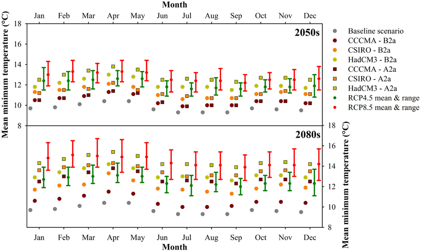
Figure 1. Mean daily minimum temperature for each month at the baseline location, according to different climate datasets: gray dots show current conditions according to the WorldClim database, brown, orange, and yellow circles (B2a emissions) and squares (A2a emissions) indicate projections with the CCCMA CGCM2, CSIRO MK2, and HadCM3 climate models, according to AR4 scenarios used in this study. The green and red dots with error bars show the means and ranges of projections from the AFRICLIM climate model ensemble (Platts et al., 2015), which uses projections from 10 General Circulation Models for the RCP4.5 and RCP8.5 radiative forcing scenarios of the 5th Assessment Report of the IPCC (2013), downscaled with five Regional Climate Models and additional statistical downscaling procedures (details on the methodology and models used are in the main text).

FIGURE 2

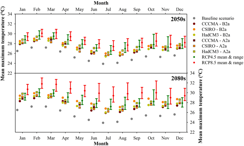
Figure 2. Mean daily maximum temperature for each month at the baseline location, according to different climate datasets: gray dots show current conditions according to the WorldClim database, brown, orange, and yellow circles (B2a emissions) and squares (A2a emissions) indicate projections with the CCCMA CGCM2, CSIRO MK2, and HadCM3 climate models, according to AR4 scenarios used in this study. The green and red dots with error bars show the means and ranges of projections from the AFRICLIM climate model ensemble (Platts et al., 2015), which uses projections from 10 General Circulation Models for the RCP4.5 and RCP8.5 radiative forcing scenarios of the 5th Assessment Report of the IPCC (2013), downscaled with five Regional Climate Models and additional statistical downscaling procedures (details on the methodology and models used are in the main text).

FIGURE 3

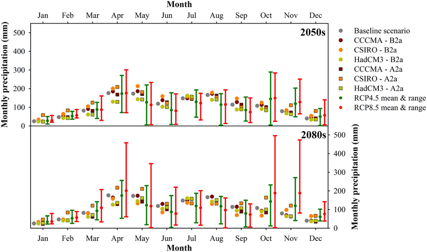
Figure 3. Total precipitation for each month at the baseline location, according to different climate datasets: gray dots show current conditions according to the WorldClim database, brown, orange, and yellow circles (B2a emissions) and squares (A2a emissions) indicate projections with the CCCMA CGCM2, CSIRO MK2, and HadCM3 climate models, according to AR4 scenarios used in this study. The green and red dots with error bars show the means and ranges of projections from the AFRICLIM climate model ensemble (Platts et al., 2015), which uses projections from 10 General Circulation Models for the RCP4.5 and RCP8.5 radiative forcing scenarios of the 5th Assessment Report of the IPCC (2013), downscaled with five Regional Climate Models and additional statistical downscaling procedures (details on the methodology and models used are in the main text).

For mean daily minimum temperatures, temperature scenarios used here covered the range of all projections of the AR5 RCP4.5, and approximately half the range of the RCP8.5 scenarios (Figure 1). For maximum temperatures, the chosen scenarios overlapped with approximately half the temperature spread of RCP4.5, while RCP8.5 generally projected higher temperatures (Figure 2). Precipitation projections varied so widely among AR5 scenarios that the chosen scenarios covered only a small part of the total range of the AFRICLIM ensemble (Platts et al., 2015).

Our scenarios thus did not cover the full range of future climates included in AR5 scenarios. However, since the objective of our study was the evaluation of the analog methodology rather than a robust climate change impact projection, use of a full climate model ensemble based on all available models was not necessary. For each climate model, we obtained projections for the A2a (business as usual) and B2a (reduced emissions) scenarios of the Special Report on Emissions Scenarios (SRES) of the Intergovernmental Panel on Climate Change (Nakicenovic and Swart, 2000). We evaluated projections for three time horizons (2020s, 2050s, and 2080s). In the CCAFS database, all data had been downscaled to 2.5 arc min resolution (~4.6 km in the study region) using the Delta method, which contains procedures for correcting for elevation, and expressed climate change relative to the WorldClim dataset for the 1950–2000 reference period (Hijmans et al., 2005).

The climate analog search was based on three climate metrics: mean monthly precipitation, mean monthly minimum temperature, and mean monthly maximum temperature. These metrics were used to compare all the grid cells within the search domain with future climates projected for the baseline location. This was done by computing “climatic distances” between places using a Euclidean distance calculation (Luedeling and Neufeldt, 2012):

Climatic distance = \sqrt (\sum_{p a r} \sum_{m} w_{p a r, m} \times {(\frac{P_{p a r, m} - F_{p a r, m}}{n o r m_{p a r}})}^{2}) ​,

in which par stands for the array of weather parameters, m is the list of all months in the year. w_{par, m} is a weighting factor to determine which of the weather parameters is given priority over the others. In this study, precipitation was assigned a weight of 2, while minimum and maximum temperatures received weights of 1. The two temperature parameters combined were thus given the same weight as precipitation, assuming both factors are of equal importance. P_{par, m} and F_{par, m} are the values for the respective parameter for the present and future scenarios and norm_par is a normalization parameter, which was set to the interquartile range of the distribution of the respective monthly values across all grid cells of the analog search domain. It should be noted that in the absence of any evidence supporting the choice of weather parameter weights or normalization method, we had to rely on researcher intuition in selecting these. It is our hope that future research will provide better guidance.

Separate climatic distance measures were calculated for each climate scenario. The grid cell with the lowest distance value was accepted as the best “matching” analog location. By using this method, a total of 18 climate analog locations (3 models × 2 scenarios × 3 time horizons) were determined for each handpicked baseline location.

For evaluating crop yield potentials, the 50 closest analog locations for each scenario, i.e., the 50 grid cells with the smallest climatic distances, were also determined. To allow for a yield potential comparison, the same procedure was also used for the baseline location, resulting in a set of 50 locations, whose current climates are similar to the current climate at the baseline site. The search domain was restricted to the area bounded by the coordinates 4° S to 4° N and 29° E to 39° E, encompassing a large part of eastern Africa.

For comparison of crop yield potentials across analog sites, all analog locations, including the additional 50 best-fit matches, were used for evaluation. For the site visits, however, resource constraints only allowed research at one site pair. For this comparison, we chose a scenario representing the 2050s time horizon as a time frame that is useful for informing land use planning processes. To raise the chance of finding interesting differences between baseline and analog sites, we decided to focus on the A2a scenario, which was the strongest of the two greenhouse gas emissions scenarios. Finally, the geographic distance between target and analog locations made us choose the CCCMA CGCM2 climate model for finding the analog location to be visited and studied in greater detail. All data processing procedures were implemented as automated functions in the R programming language (R. Development Core Team, 2011).

Potential Crop Performance Comparison

The agro-ecological potential for major crops was compared between target and analog locations based on global maps of crop production potentials included in the Global Agro-ecological Zones dataset published by the International Institute for Applied Systems Analysis (IIASA; Fischer et al., 2012). In accordance with production methods at the baseline location, yield potential in this analysis was defined as the potential yield under low-input rainfed conditions, as represented in IIASA's datasets. We chose the data layers for yields of low-input rainfed cultivation of maize and coffee, two major crops of the study area. Crop yields in this dataset account for climatic, edaphic and to a limited extent socioeconomic constraints (availability of irrigation and inputs) to crop production. For each climate scenario, each of these layers was sampled at the best-fit analog location, as well as at the 50 grid cells with the smallest climatic distances. According to the rationale of the climate analog approach, the crop potential values obtained for the best analog location should provide estimates of future yield potentials at the baseline location. We preferred IIASA's dataset over alternative sources, such as Monfreda et al. (2008), because it explicitly accounted for climate and soil conditions, which we considered crucial for our mountainous study region.

Investigation of the distribution of climatic distance values for the grid cells of the analysis revealed that for most climate scenarios, many cells had similarly low climatic distances. Yield potentials at all, or most, of the 50 closest analog locations (the 50 cells with the lowest climatic distance values) should thus reflect future prospects for the baseline location. If the analog method works as is commonly assumed, these yield potentials should be quite similar, especially if they are based on similar assumptions, such as low inputs and rainfed conditions. If yield potentials vary widely among these 50 locations, the value of the analog sites for projecting future yields must be doubted. This is particularly true, where yield potentials at the closest analog sites are not representative of yield conditions among the 50 climatically most similar locations.

Local Ecological Knowledge

Qualitative local knowledge on local farming systems and climatic effects on crop production was collected using the knowledge-based systems methods (Walker and Sinclair, 1998; Dixon et al., 2001). First, a short one-week scoping study was undertaken to provide the initial site characterization and to explore whether sufficient scope existed for further study of both sites and comparison between them.

According to Walker and Sinclair (1998) the scoping stage of the study is the best time to further design a detailed “knowledge acquisition strategy,” which involves defining criteria for selecting appropriate strata among informants and purposively choosing informants from both locations. The criteria were: (1) the farm had to be positioned within the grid cell corresponding to each location; (2) the farm had to be managed by a smallholder farmer representative of the local general farmer population in terms of farm size; and (3) the informant had to have lived for more than 15 years within the study area. Such long-term presence was required to ensure farmers' ability to report on local weather phenomena—knowledge that can only be obtained during many years of farming experience at the respective site. Selecting the right stratum, the right “layer” of the general population of potential informants fitting the criteria, ensures just the knowledge of the people of interest to the study is obtained and a successful comparison can be executed.

A total of 20 different informants were initially interviewed via a local translator, using semi-structured interviews with topics covering local socio-economic conditions, farm management strategies and their relation to local climate conditions and extreme weather, pest and disease occurrence, and locally observed changes in climate conditions. The informants included both men and women, who in most cases were over 50 years old. Some informants were accompanied by one or two family members contributing to the interview. In this study, such a setting is regarded as an interview with one informant. Detailed knowledge was gathered via additional interviews with nine of the original 20 farmers, who were randomly selected. Repeating interviews with the same participants was important for obtaining deeper explanatory knowledge and for resolving inconsistencies. Feedback sessions were held with a wider section of the communities at both sites (analog n = 17, baseline n = 42) at the end of the knowledge acquisition stage. By inviting all the informants and their families to these meetings we ensured that gathered local knowledge could be “tested” with the wider community, thus allowing for the identification of local common knowledge, knowledge that can be assumed to be held by most, if not all, within the community. The feedback sessions also allowed us to report our findings back to the community and to clarify any misconceptions and conflicting issues.

Results

Climate Analogs

Reasonably well-matching climate analogs were found for all climate scenarios. Figure 4 shows, for the baseline location, current climate conditions (black lines) as well as projected conditions for the 2050s time horizon and the A2a emissions scenario for all climate models (dashed green, blue, and red lines). These are compared with current climate conditions at the best-fit analog locations for all climate scenarios (solid lines). Similar figures for all other climate scenarios are provided as Supplementary Materials (Figures S1–S5). The greatest deviations between projected climate at the baseline and current climate at analog locations were found for precipitation, while correspondence was high in most months for both temperature metrics. For all climate scenarios, the 50 closest climate analogs had climatic distances from projected conditions at the baseline site below 0.22 (Figure 5). Within climate scenarios, differences in the climatic distance among these 50 sites ranged between 0.02 and 0.07, indicating fairly similar conditions within these groups of sites.

FIGURE 4

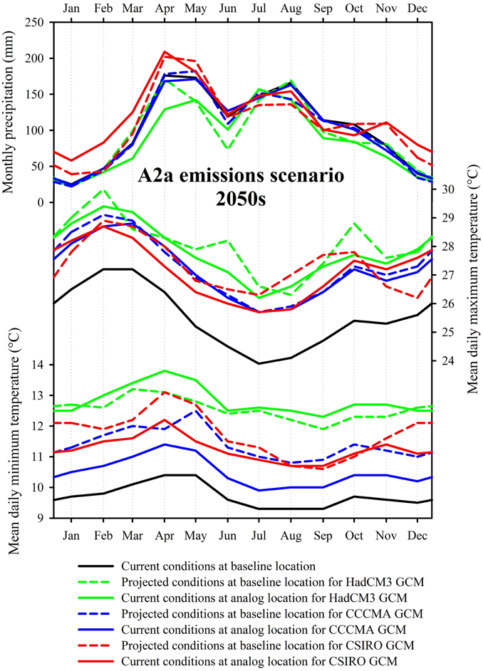
Figure 4. Distributions of monthly precipitation, mean daily maximum, and minimum temperatures derived from the WorldClim and CCAFS databases. Data are shown for the current climate of the baseline location, projected climate at the baseline location, and current climate at analog locations corresponding to projected futures according to three climate models, for the A2a greenhouse gas emissions scenario and the 2050s projection horizon.

FIGURE 5

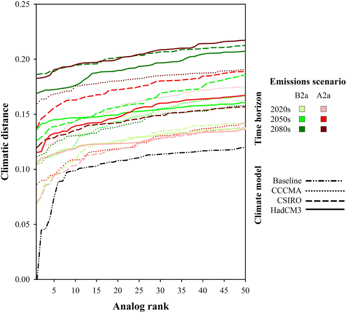
Figure 5. Distribution of climatic distances between the 50 closest climate analog locations and the projected conditions for the baseline site for 18 climate change scenarios, and a baseline scenario. A horizontal line and a low climate distance value would indicate that the 50 analog locations have almost identical climate conditions.

Climate analogs for the various climate scenarios were distributed between 6 and 120 km from the baseline location (Figure 6). Analogs were clustered in the valley south of the baseline site, where eight of the 18 analogs were located, as well as in an area about 50 km north of the baseline site, on both sides of the Kenya-Uganda border, where five sites were located. Five further analog sites were situated to the south-west of the baseline location, on the Southern slope of Mt. Elgon (1 site), and approximately 110–120 km southeast of Mt. Elgon (4 sites).

FIGURE 6

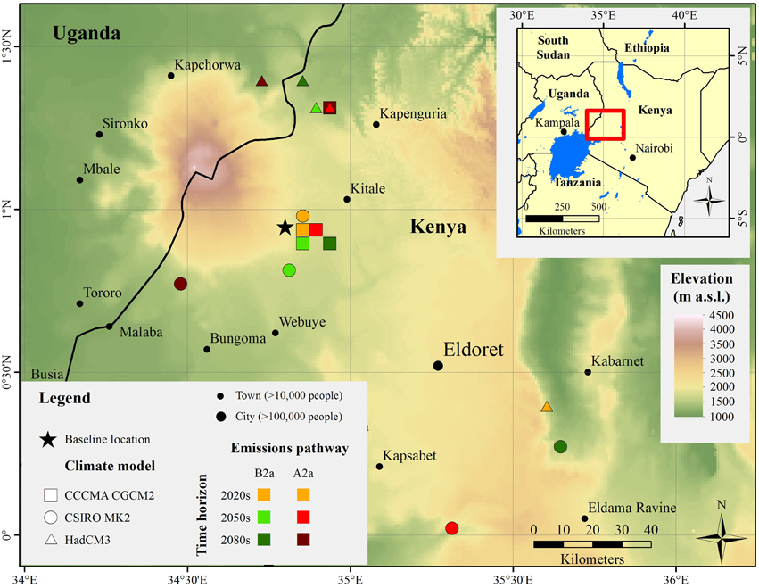
Figure 6. Location of climate analogs corresponding to climate projections for two greenhouse gas emissions scenarios, three time horizons, and three climate models, along with the location of the baseline location. The analog location used for the site comparison is represented by the red square (CSIRO MK2, A2a, 2050s). Inset: location of the study area in Western Kenya. Note that analog locations for the 2020s scenarios are co-located among emissions scenarios for all climate models and therefore not distinguished by different colors. Shading indicates elevation above mean sea level, according to the GTOPO30 dataset (USGS, 1996).

Crop Yield Potentials at Baseline and Analog Sites

Crop yield potentials according to IIASA's projections (Fischer et al., 2012) varied substantially between climate analogs corresponding to different climate scenarios (Figures 7, 8). Assuming effectiveness of the analog approach in selecting 50 analog sites that each represent the future conditions of the baseline location, this would indicate that climate change impacts on crop yields are highly uncertain. Figures 7, 8 show yield potentials for maize and coffee at climate analog locations of the baseline site, for all 18 future climate scenarios. For both crops, projections were consistent among the 2020s scenarios, for which expectations of relatively small changes were confirmed, but varied strongly for scenarios corresponding to the 2050s and 2080s. Following the climate analog logic, this would indicate that prospective yields depend strongly on which of the projected future climates materializes. While this may be the case, the level of variation implied by the analog analysis greatly exceeded the range of uncertainty about future yield changes in tropical regions reported by the IPCC's 5th Assessment Report (Porter et al., 2014), where yield change rates are estimated at between approximately −4 and +3% per decade. Extrapolation of the extremes of this range toward 2080s scenarios would result in yield changes between about −30 and +25% (and −19 to +15% for the 2050s). Comparing baseline maize yields with yields at analog locations frequently produced estimates that were far outside these ranges (Figure 7). Thornton et al. (2010, 2011) also reported much less uncertainty about future yields for East Africa than implied by the analog comparison, even for high-end warming scenarios. Likewise, a meta-analysis by Challinor et al. (2014) produced much narrower confidence intervals for climate change impacts in low-latitude maize yields than the analog comparison suggested. For warming scenarios of up to 6–8°C, Rosenzweig et al. (2014) projected yield losses for maize at low latitudes of up to 60%, which comes close to yield losses implied by the analog comparison. However, the extremes of this range probably stem from non-linear effects of very high temperatures (Lobell et al., 2011), which are unlikely to be of major importance at the high elevation of the study region.

FIGURE 7

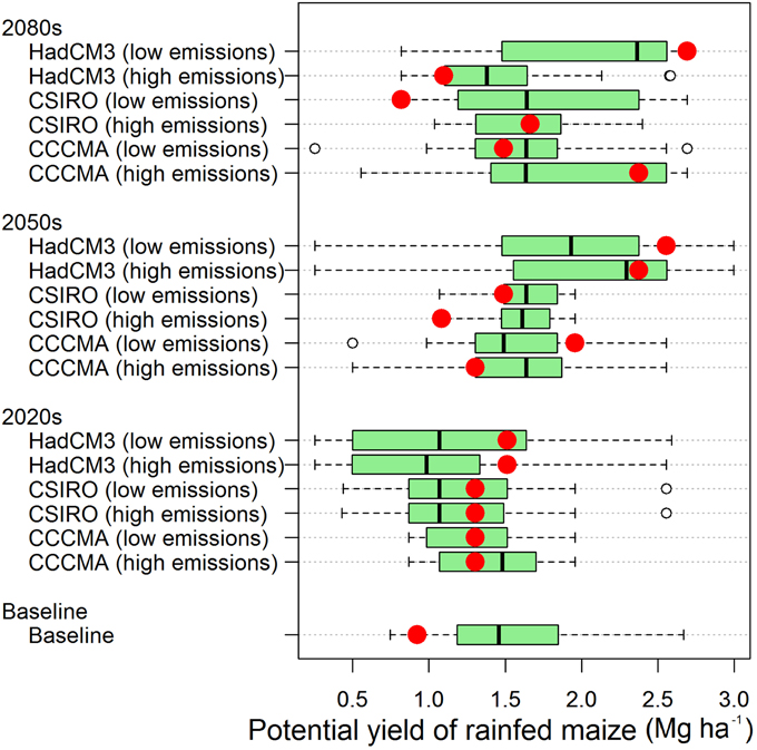
Figure 7. Distributions of maize yield potentials among 50 candidate climate analog locations of the baseline site on Mt. Elgon, Kenya, for each of 18 future climate scenarios. The 50 sampled sites are those grid cells where the current climate was most similar to the projected future climate at the baseline location, for the respective climate scenario. Low emissions refers to the B2a and high emissions to the A2a greenhouse gas emissions pathway. Red dots mark the closest analog.

FIGURE 8

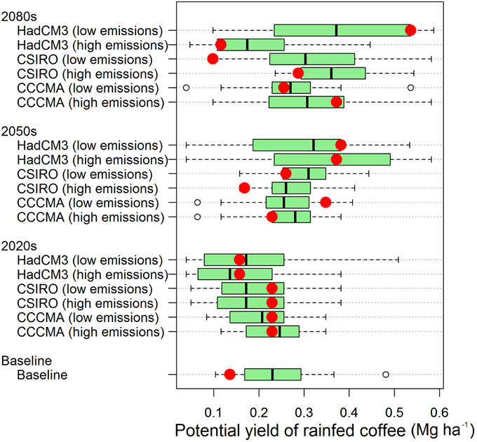
Figure 8. Distributions of coffee yield potentials among 50 candidate climate analog locations of the baseline site on Mt. Elgon, Kenya, for each of 18 future climate scenarios. The 50 sampled sites are those grid cells where the current climate was most similar to the projected future climate at the baseline location, for the respective climate scenario. Low emissions refers to the B2a and high emissions to the A2a greenhouse gas emissions pathway. Red dots mark the closest analog.

Interestingly, the crop yield dataset indicated low current yield potentials for both crops at the baseline location, with increases likely in most climate change scenarios. Current yields at the baseline location were also low compared to average countrywide yields reported in the FAOSTAT database (FAO, 2014). Between 2000 and 2011, these varied between 1.3 and 1.9 Mg ha⁻¹ for maize and between 0.2 and 0.6 Mg ha⁻¹ for coffee. These numbers are well-aligned with estimates by Monfreda et al. (2008), who reported yields of 1.9 Mg ha⁻¹ of maize and 0.22 Mg ha⁻¹ of coffee for the baseline location. IIASA's dataset indicated yield potentials of only 0.92 Mg ha⁻¹ for maize and 0.14 Mg ha⁻¹ for coffee under low input rainfed conditions at the baseline location. These low yield potentials are likely a reflection of the location of the baseline site on the mountain slope, where current conditions may be cooler than optimal for many crops. However, among the 50 grid cells with similar climate to the baseline location, yield potentials were higher, averaging 1.5 Mg ha⁻¹ for maize and 0.24 Mg ha⁻¹ for coffee. This may suggest that the global IIASA dataset underestimated yield potentials, possibly by overemphasizing negative impacts of elevation.

Projected yields were inconsistent within the populations of close analog locations corresponding to all climate scenarios. Likely maize yields across the 50 closest analog sites, as indicated by the interquartile range of the distributions (shown by the boxes in Figures 7, 8) varied by between 0.5 and more than 1 Mg ha⁻¹ for many climate scenarios, which was similar in magnitude to the largest differences between mean crop yield potentials among climate scenarios (Figure 7). Coffee yield potentials showed similar patterns (Figure 8). This finding implies that the impression of likely climate change impacts that the analog comparison generates depends strongly on which candidate analog site from among the 50 climatically similar locations is chosen for analysis. Many of the best-fit (smallest climatic distance) analog sites were not representative of the population of close analogs, based on yield potentials for maize and coffee. These values are indicated by the red dots in Figures 7, 8. Location of these dots near the extreme ends of the illustrated yield potential distributions indicates that the yield potential at the closest analog location is different from yield potentials at most climatically similar sites.

Site Comparison

One climate analog location was chosen for more detailed comparison with conditions at the baseline site, which is locally known as Muroki. Among the three climate analog locations representing the 2050s time horizon for the A2a emissions pathway, we chose the site corresponding to the CCCMA CGCM2 climate model, because it was geographically closest to the baseline location. Figure 9 shows the climatic distance between projected climate conditions for the chosen climate scenario and grid cells surrounding Mt. Elgon, as well as the locations of baseline and analog locations. Besides facilitating study logistics, the choice of an analog site that was close to the baseline location was also expected to minimize non-biophysical differences between baseline and analog sites, such as those related to market infrastructure or cultural preferences (our results showed, however, that this expectation was not met). The location that was selected (0°56.25′N; 34°53.75′E, at approximately 1798 m above sea level) is locally known as Bituti and located approximately 10 km to the east and 200 m lower in altitude compared to the baseline location (0° 56.25′N; 34° 48.75′E, at approximately 1998 m above sea level). Both locations were close to a main road. The analog location is approximately 16 km closer to the town of Kitale. The baseline location included a small hamlet with a few shops and a gas station.

FIGURE 9

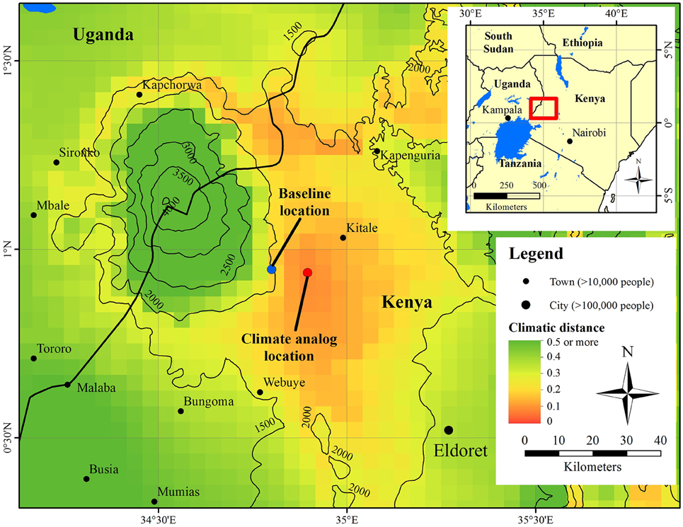
Figure 9. Distribution of the climatic distance between all grid cells around Mt. Elgon, Kenya, and the projected climate at the baseline location for the 2050s, according to the CCCMA CGCM2 climate model driven by the A2a greenhouse gas emissions scenario. The climatic distance is minimized at the site designated as Climate analog location. Thin black lines are elevation contour lines based on the GTOPO30 dataset (USGS, 1996).

Agricultural Systems at Baseline and Analog Sites

Smallholder farmers were found in both the baseline and analog location, but land use history and land distribution differed markedly. Most farmers at the baseline location bought their farms from European settlers after Kenya's independence in 1963. Average farm size was around 7 hectares (Table 1), with narrow fields laid out along contour lines and separated by old erosion control structures. The most important crops grown were maize (mostly the hybrid varieties “H614” and “H6213'), beans, tomatoes, coffee, tea, and Irish potatoes. Farmers considered the relatively cool local climate conditions on the mountain slope as beneficial for growing tomato, coffee, tea, and Irish potato, but not very suitable for beans. Tea was found either intercropped with maize or in monoculture. Smaller vegetable fields were cultivated to supplement household nutrition and women's income. Crops grown here included Collard Greens, kale (Sukuma Wiki), cowpea (Kunde), cabbage, banana, sorghum, millet, sweet potato, spider plant (Saga), pumpkin, cassava, arrowroot, spinach, carrot, sunnhemp (Miro), amaranth (Dodo), and sugar cane, although not every farmer grew all these crops. Around half of the vegetables produced on these fields were sold on local markets. Fruit trees, such as avocado, loquat, mango, white sapote, and guava, were grown around the homestead. Farmers owned between three and six head of cattle, along with some goats, sheep, donkeys, and poultry. Soils at the baseline location were reported to be of volcanic origin, dark brown, or blackish and mostly of loamy texture. This field observation was inconsistent with data in the relatively coarse-grained KENSOTER database (Kempen, 2007), which describes soils at this location as Rhodic Nitosols.

TABLE 1

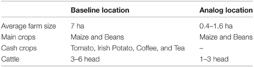
Table 1. Site characteristics at the baseline and analog locations.

Smallholder farms at the analog location were much smaller in size, with households only cultivating between 0.4 and 1.6 hectares of land (Table 1), nearly all of which was allocated to maize (mainly varieties “H614” and “H6213”) and beans. Vegetables and fruits for home consumption were grown in small kitchen gardens and at the boundaries of the homestead. The garden vegetables and fruits grown at the baseline location were also grown in the analog location, although at a smaller scale. Smallholder farms at the analog location were situated between very large holdings, some of which were reported to comprise more than 1200 hectares. Major activities of these large farms were the production of maize seeds, both hybrid and regular, for national seed companies, along with maize for the national consumption market. These commodities were produced with relatively high inputs and mechanized production methods, such as aerial spraying of pesticides from planes. Smallholder farmers occupied steeper plots and other marginal lands, on which they raised between one and three head of cattle and some poultry for home consumption. Donkeys, goats, or sheep were not often observed or reported. A wider range of soils was reported compared to the baseline site. Soils were reddish in color, considered less fertile than those at the baseline site and included clay, sandy loam, clay loam, and sandy soils. This description is consistent with the classification as Haplic Ferralsol by the KENSOTER database (Kempen, 2007).

Biotic Constraints

Changes to biotic constraints are a likely consequence of climate change (IPCC, 2013; Falloon et al., 2015), and changes in geographic distributions of pests, weeds, and pathogens (Bebber et al., 2013; Berzitis et al., 2014; Sparks et al., 2014) and the number of generations per year (Ghini et al., 2008; Luck et al., 2011; Luedeling et al., 2011) have been projected for many biotic stressors. Due to the strong climate response of many pests and pathogens, one might expect pest, weed and disease pressure to differ between baseline and climate analog locations.

Local climate at both locations manifested itself in a range of biotic constraints. Comparing how these affect the agricultural system at both sites may help assess what farmers at the baseline location might face under future climate conditions. The spectrum of reported pests and diseases showed no difference between the baseline and analog sites when it concerned crops both sites shared. Blight was seen as the biggest problem at both locations, where it affected beans, tomatoes, and Irish potato, and severely reduced yields of avocado and coffee. The general term “blight” is used locally for all these incidences, but it was clear to farmers that different crops contracted different types of blight. Blight infection was reported to be most severe during foggy, humid, and cold conditions. The strength of this association is illustrated by the dual use of the local word Barafu, which means blight, as well as cold, ice, or fog. Farmers at both locations reported difficulties in accessing fungicides against blight. Other reported diseases were maize smut (most likely Ustilago maydis) and Maize Streak Virus (MSV). The spreading mechanism of MSV, which is disseminated via insect hosts, was not known to interviewed farmers. Although observed in both locations, this disease did not appear to have a major negative impact on yields, and farmers did not associate its occurrence with local weather conditions.

Stalk borer was reported as the most significant pest in maize and it was mentioned by all farmers; it was estimated to reduce maize yields by about 10% at both locations. Stalk borer was reported to infest maize plants before they start to flower, and to become a serious pest as soon as precipitation is low and temperatures are high for a week or two. The short dry period that typically occurs during the month of June appears to be when most stalk borer infections take place. Other pests, such as army worm (Spodoptera exempta), cutworm (Agrotis spp.), aphids and whiteflies, American bollworm (Helicoverpa armigera), spider mites (Tetranychidae spp.), and a more generally used “Caterpillars” are considered serious problems for a range of crops. For all crops grown in both locations, the same pests were observed at both sites. Among all these pests, stalk borer was clearly considered most damaging. High infestation by all pests was associated with low precipitation combined with high temperatures at some point during the growing season. Weevils (Sitophilus zeamais) were a feared storage pest destroying stored maize during the long dry period, between December and March. Although extensive attention was given to the pest and disease occurrence at both sites, no clear differences could be identified. Farmers at both locations reported an increase in pest occurrence, but the study did not allow for a quantitative analysis of pest pressure differences between the two locations.

Climatic Constraints

Several weather phenomena were reported to negatively affect local crop production at both sites, including hailstones, fog, wind, intense rainfall, and unexpected dry spells during the growing season. Hailstones were assigned particular importance due to their potential to destroy young plants completely or severely reduce the production of already established crops (especially garden vegetables, beans, tomatoes, and potatoes). Hailstones reportedly occurred between 2 and 4 times a year, during the months of April to August, but did not affect all farms every year. Maize that was scarred by hailstones was observed at both locations. Fog was considered a severe problem because of its connection with blight infection. High wind was associated with lodging of maize at both the analog and baseline sites. Lodging during the pollination stage leads to poor pollination, resulting in low yields. Very intense rainfall led to waterlogging, erosion, and leaching of applied chemical fertilizers. Waterlogging was a bigger problem at the baseline location, especially at sites where roads and tracks drain onto old terraces. Farmers reported an increase in rainfall intensity and unexpected short dry spells during months previously expected to generate light rain and low temperatures every day. These dry periods during the growing season were associated with outbreaks of pests and reduced pollination of both maize and beans. Dry weather during pollination was reported to make beans shed their flowers, while maize pollination was claimed to be more successful during light drizzle than under hot and dry conditions, which greatly reduce pollen vitality. Since only monthly temperature and precipitation data were used for determining analog locations, the search procedure was unable to account for most of these site-specific weather phenomena.

Socioeconomic Constraints

Besides being limited by climatic constraints, crop production as well as food and income security were also limited by a range of socio-economic factors at both locations. Availability of capital to invest in certified seeds, chemical fertilizer, pesticides, fungicides and labor were named as just as important for a successful harvest as favorable weather, at both locations. Farmers at the analog location experienced more difficulties in acquiring the required inputs. Seeds of appropriate varieties and other inputs were not always available on the local market at either location. Income from crop production, and the security associated with it, was also dependent on access to markets, quality of the roads during harvest season, and the ability to store maize and chemically protect it from weevils. Farmers at the baseline location appeared to be in a better position to deal with environmental shocks or economic setbacks, due to their more diverse farming system and larger resource base in the form of livestock and cash crops.

Discussion

Location of Climate Analogs

Most climate analogs were situated in close proximity of the baseline location (Figure 6). Such a setting should facilitate use of analog sites as learning locations, and it seems reasonable to expect that cultural or infrastructural similarities between the sites should enable meaningful exchange of ideas and technologies. The close association of baseline and analog sites is due to the strong elevation gradient in the region, with the baseline site on the slope of Mt. Elgon and most of the analog sites located a few 100 m lower in elevation. Depending on rainfall, climate analogs were on different sides of the mountain, with analogs for dryer climate scenarios tending to lie north of the mountain, while wetter analogs were to the east and south.

Evaluation of Potential Yield Datasets

One of the main rationales for using the climate analog approach is that its use could facilitate the projection of climate change impacts on farms and the identification of promising options for adaptation (Ramirez-Villegas et al., 2011). Among the most commonly used indicators of agricultural performance are the yields of staple crops such as maize or cash crops such as coffee. The projection of yield changes has therefore been at the center of most efforts to project the impacts of climate change with process-based models (Jones and Thornton, 2003; Marin et al., 2013; van Wart et al., 2013). Yield potentials determined with the analog approach did not paint a conclusive picture, varying strongly among climate scenarios, and equally strongly among the 50 locations that were most similar to the analog location, according to the climatic distance metric (Figures 7, 8). Among the likely reasons for this variation are differences in soils and crop management. If actual yields rather than modeled yield potentials were compared, differences in socio-economic and cultural settings would contribute additional variation. This indicates that the analog approach did not only fail to provide a clear indication of the magnitude of climate change impacts across climate scenarios; it also did not succeed at consistently predicting the magnitude, or even direction, of change within any particular scenario.

Evaluating yield potential differences at the best-fit analog location in the context of those across the 50 most climatically similar locations emphasized the risk attached to choosing one analog location to represent the climatic future of a site for a particular climate scenario. Many such best-fit climate analogs were not representative of yield potential levels indicated by the larger sample of 50 climatically similar points. If such a site is assumed to represent climate impacts, but most settings that are climatically similar to this location would have very different potentials, substantial errors could result, which might lead to poorly directed adaptation processes. The large variation in yield potentials among locations with similar climate implies that a substantial number of analog candidate sites would have to be sampled, in order to gain a conclusive picture of likely future changes. Since actual visits to analog locations are not just a data processing exercise but might incur substantial costs, such large sample sizes might be prohibitive in most cases, leaving adaptation planners with great uncertainty about how representative a selected analog location is of future climate change impacts.

An interesting finding was that for most climate scenarios, yield potentials were not expected to decline, but rather showed a tendency to increase over time. This result contradicts widespread expectations of climate change impacts, in which negative implications typically take center stage (Schlenker and Lobell, 2010; Thornton et al., 2011; IPCC, 2013; Challinor et al., 2014; Rosenzweig et al., 2014). However, such projected increases might be realistic, considering that temperatures on the mountain slope are in fact quite cool and probably below the growth optimum for many crops most of the time, especially at night, as findings by Thornton et al. (2009) confirm.

Site Comparison

The first important insight that was gleaned from the site comparison between baseline and analog locations was that climatic hazards affected agricultural production at both sites, but these hazards were only indirectly related to the climate variables used in the analog search procedure. The most serious weather condition that directly affected crops was hail, a phenomenon whose response to changes in precipitation and temperature is not well understood (Mahoney et al., 2012; Hermida et al., 2013). Other weather conditions had indirect effects, through impacts on pests and diseases. These conditions were fog, as well as short dry spells during the growing season that enabled development of fungal diseases and insect pests, respectively. All these climatic hazards constitute fine-scale phenomena that cannot directly be obtained from GCM-derived climate scenarios with a monthly resolution, such as the ones used in this study. Such events are therefore not captured well by the site comparison. It seems likely that especially hail and fog are microclimatic situations that specifically occur on the mountain slope. Using a valley bottom location as an analog would then not provide much guidance on how to cope with such challenges or allow projection of the frequency of their occurrence in the future. It is also noteworthy that any change in rainfall intensity, and its associated impacts, cannot be anticipated using climate analog modeling, at least not with the climate metrics considered in this study. Total precipitation, as calculated using monthly averages, might remain the same in the future, even though changes in the diurnal distribution of rainfall events might adversely affect farms.

Regarding cropping systems, farms at the baseline and analog locations had many similarities. The staple crops that were grown were similar (maize and beans), and farms at both locations also cultivated vegetables for home consumption. Climate did not seem to be a major constraint to any of these crops. All crops were also affected by the same pests and diseases, indicating that farmers are struggling with similar problems at both sites.

However, some differences between sites existed. Coffee and tea were only found at the baseline location, while they were absent from farms at the analog site. Yet the reason for this difference did not seem to be of climatic nature, but rather the small farm sizes at the analog site, which did not allow farmers to spare land from the cultivation of staple crops. The marginal nature of the land farmers cultivated there may not have allowed successful cultivation of these cash crops. In this context, it is also noteworthy that coffee and tea at the baseline location were likely legacy crops that had been grown by European settlers before the current owners acquired the farms.

Limitations of the Climate Analog Approach

As stated in the Section on Climate Analogs, the usefulness of the climate analog method to assist in the projection of climate impacts and in sourcing adaptation options hinges on the assumption that climate is the main cause of variation among farms. Our analysis sheds doubt on this assumption. Potential crop yields among candidate analog locations under low-input rainfed conditions varied widely, even though these sites had very similar climates, indicating that other factors are of critical importance for determining yield levels. The IIASA methodology that produced this dataset used non-climatic production constraints, most notably edaphic factors (Fischer et al., 2012), that are likely responsible for this variation. The site comparison also indicated some problems with the main premise of climate analog analysis. Even though the baseline and analog locations were only about 10 km apart, smallholder farms differed in a number of critical respects, which severely constrained the usefulness of comparing these sites. Of course, differences are not always as significant as those between a mountain slope and a valley bottom location observed here. Yet, there are always likely to be some important non-climatic differences within any set of two locations, and analysts of climate analogs must gain awareness of such differences before beginning to interpret differences between sites as climate change impact indicators.

It would of course be possible to include more variables into a climate analog search. In theory, a search procedure could include additional climate variables, such as the length of dry spells, rainfall extremes, or hail risk. Daily climate projections could be mined for a host of additional variables. Likewise, other environmental variables, such as soil conditions or natural vegetation type, or socioeconomic variables like distance to market, land tenure regime, or household income could be added to the search. There may thus be some potential in raising the complexity of the search algorithm for enhancing the usefulness of analogs for adaptation planning. However, for any additional variable that is included in the search procedure, one would have to know the future status at the baseline location, and have a gridded dataset for the present situation. For example, for household income to be included, a projection of future household income would be needed, and for inclusion of the length of dry spells, a gridded dataset of this variable for the entire search area would be required. In practice, few variables may therefore qualify for inclusion in the search procedure.

Even if more variables could be included in a search procedure, and even if such variables were to cover some aspects of the sites' socio-economic and cultural settings, uncertainty about the causes of land use differences would remain. The array of drivers that shape agricultural systems is simply too broad for complete representation in an analog search procedure. Examples of factors that may have to be included are the cultural preferences of local people, the existence of markets for certain products, availability of financial, or human capital or the land tenure regime. Comprehensively listing all the factors that may be important would be a very challenging exercise, and including all the factors on such a list in an analog search procedure may well be impossible. It is also worth mentioning that system evolution over time is strongly path-dependent, meaning that its current state results not only from the drivers that currently affect the system but also from a long series of decisions made in the past. In practice, all these influences on the current state of the system make it very difficult to be confident that an identified analog location is really a useful learning site for informing adaptation at the baseline location. This problem is particularly severe, when study resources are insufficient for analysing a large number of potential analog locations, which may often be the case. Especially if only one potential analog location is evaluated, chances are high that current practices at this location would not be useful for future application at the baseline site.

Climatic differences between present and future scenarios become greater with lengthening time horizons. Temperature increases projected by the 2080s are much greater than those expected by the 2020s, and it thus seems likely that climate will explain a larger proportion of the differences between baseline and analog sites corresponding to more distant time horizons than for nearer ones. This principle appears to apply for predictive models in general (Vermeulen et al., 2013). There may thus be some scope for sourcing adaptation options for the far future from such comparisons, but for most decision-makers the 2080s may not be a time horizon worth considering at this point. In the analog case tested in this study, and likely in many other situations (e.g., Nyairo et al., 2014), climatic differences appeared to explain only a small part of the variation between sites, while other “noise” factors were more significant. This severely restricts the usefulness of the analog approach for projecting climate impacts on agricultural systems.

More Promising Uses of Climate Analogs

There may still be much to be gained from applying the analog approach, but there are more promising applications than projecting climate impacts on man-made systems or adapting such systems to climate change. We suspect that the approach would be much more successful in natural ecosystems, which change more slowly and are shaped to a greater extent by climatic and environmental factors than agricultural systems that are driven by a host of “messy” socioeconomic factors (for example, see Ford et al., 2010; Feeley and Rehm, 2012). In theory, it may also be possible to extend an analog search procedure to include such factors, but this may hardly be feasible in practice, because no datasets of such factors exist at adequate resolutions and coverage.

There is also scope for using the analog approach for the development or validation of models of plant physiology or other ecological phenomena that are also impacted by climate change. For many such phenomena, existing models lack credibility, because they were developed under current (or past) climatic conditions, such that any use on future scenarios may constitute an impermissible extrapolation. The existence of climate analog locations allows collection of data in climates that resemble those of the future, and they also offer opportunities for validating impact projections obtained with process-based models. Such an approach has been proposed for improving winter chill models for temperate fruit trees (Luedeling, 2012).

Climate analog locations may also be useful for agricultural systems, mainly in the development of new crop varieties and tree cultivars (Falloon et al., 2015). Given the pace of climate change in some parts of the world, testing crop performance in the place where their cultivation is envisaged may no longer be sufficient for ensuring successful cultivation in the future, especially for long-lived organisms such as trees. Using climate analog sites as additional testing grounds, or for guiding germplasm selection, may be advisable for extending the validity of models into a warmer future. In this application, as in essentially all other uses of the analog approach, consideration of non-climatic site parameters is advisable, if not required. Factors such as soil type or hydrological features for natural ecosystems, and in addition aspects of the socioeconomic environment for agricultural settings, should be as similar as possible between baseline and analog sites. Ensuring this, however, will likely require considerable exploratory work in almost all cases, taking away from the simplicity of the approach that makes up a large part of the appeal of the analog method.

Conflict of Interest Statement

The authors declare that the research was conducted in the absence of any commercial or financial relationships that could be construed as a potential conflict of interest.

Acknowledgments

We are grateful to The Rockefeller Foundation (Grant # 2011 CRD 306) for funding the AdaptEA project (led by the Centre for International Forestry Research; CIFOR), within which this study was conducted. We also acknowledge support from the CGIAR Research Programs on Climate Change, Agriculture and Food Security (CCAFS), as well as Forests, Trees, and Agroforestry (FTA), and from Bangor University. The field work conducted in this study would not have been possible without logistical assistance from Vi-Agroforestry in Kitale, Kenya, or without the help of Joseph Muse, who acted as guide and translator in the field. We are indebted to all farmers who participated in our interviews, without whose contributions this study would have been impossible. Finally, we are grateful for constructive reviewer comments, which greatly helped improve the manuscript.

Supplementary Material

The Supplementary Material for this article can be found online at: http://journal.frontiersin.org/article/10.3389/fenvs.2015.00065

Figure S1. Distributions of monthly precipitation, mean daily maximum, and minimum temperatures derived from the WorldClim database. Data are shown for the current climate of the baseline location, projected climate at the baseline location, and current climate at analog locations corresponding to projected futures according to three climate models, for the A2a greenhouse gas emissions scenario and the 2020s projection horizon.

Figure S2. Distributions of monthly precipitation, mean daily maximum, and minimum temperatures derived from the WorldClim database. Data are shown for the current climate of the baseline location, projected climate at the baseline location, and current climate at analog locations corresponding to projected futures according to three climate models, for the A2a greenhouse gas emissions scenario and the 2080s projection horizon.

Figure S3. Distributions of monthly precipitation, mean daily maximum, and minimum temperatures derived from the WorldClim database. Data are shown for the current climate of the baseline location, projected climate at the baseline location, and current climate at analog locations corresponding to projected futures according to three climate models, for the B2a greenhouse gas emissions scenario and the 2020s projection horizon.

Figure S4. Distributions of monthly precipitation, mean daily maximum, and minimum temperatures derived from the WorldClim database. Data are shown for the current climate of the baseline location, projected climate at the baseline location, and current climate at analog locations corresponding to projected futures according to three climate models, for the B2a greenhouse gas emissions scenario and the 2050s projection horizon.

Figure S5. Distributions of monthly precipitation, mean daily maximum, and minimum temperatures derived from the WorldClim database. Data are shown for the current climate of the baseline location, projected climate at the baseline location, and current climate at analog locations corresponding to projected futures according to three climate models, for the B2a greenhouse gas emissions scenario and the 2080s projection horizon.

References

Asseng, S., Ewert, F., Rosenzweig, C., Jones, J. W., Hatfield, J. L., Ruane, A. C., et al. (2013). Uncertainty in simulating wheat yields under climate change. Nat. Clim. Change 3, 827–832. doi: 10.1038/nclimate1916