 Lina M. Moreno-Conn*
 Nubia S. Rodríguez-Hernandez
 José Orlando Arguello
 Oscar Gallo Gordillo
 Jaime H. Bernal-Riobo
 Miguel ArangoJosé E. Baquero
- Agricultural Research Group, Colombian Agricultural Research Corporation—Agrosavia, La Libertad Research Center, Villavicencio, Colombia
Increasing cultivation on acid soils of Colombia’s Eastern High Plains in the Orinoquia region require crop management strategies that balance commercial and environmental interests. Previous research showed the effects of land preparation and management on certain aspects of ecosystem services of these acid soils. This research aimed to comprehensively evaluate the impact of use and soil management in a native savanna Oxisol converted to five production systems gaining traction among local farmers: Annual crops rotation–sugarcane (ACR-S); Annual crops rotation-maize-soybean (ACR-MS); Sugarcane monocrop (SM); Rubber associated with Desmodium ovalifollium (R-Do) as a cover crop; Pasture Brachiaria decumbens - Annual crops rotation (PBd-ACR) and native savanna (NS) as a control. The experimental design consisted of conditioning the soil with two doses of dolomitic lime and incorporating three tillage methods over 5 years. A Principal Components Analysis (PCA) constructed indicators of ecosystem services (ES), such as fertility, water regulation, macroinvertebrate diversity, climate control related to greenhouse gas emissions (GHG) and carbon stock. The indicator values were adjusted between 0.10 and 1.0. Physicochemical variables with the greatest statistical weight were identified for components 1 and 2 each year. The fertility indicator of the native savanna for year one had a low range with a value of 0.11 compared to the other systems (p ≤ 0.05). During the years two, three, and four, soil fertility increased in the PBd-ACR (0.51) production system compared to the other systems. PBd-ACR generally improved water supply, although with lower indicator values than ACR-MS and R-Do. PBd-ACR show high biodiversity for edaphic macroinvertebrates compared to other systems. Field measurements detected methane emissions only in the SM system. Oxisols changed with the introduction of crops. The positive and negative tradeoffs of production systems and their agronomic practices should be considered in agricultural development of these acid soils.
1 Introduction
The rapid increase in world population, growing demand for food, and urban and agricultural expansion have been the key driving forces for land-use change (Yu et al., 2013). Anthropogenic land surface change converts natural savannas and forests into cultivated lands for food, fiber, raw materials, and bioenergy (Alexander et al., 2015). These systems can negatively impact ecosystems and environmental services, contributing to environmental degradation and global climate change (Foley et al., 2005; Lawler et al., 2014; Tolessa et al., 2017; Hasan et al., 2020).
Soils are of vital importance for the support, provision, and regulation of many ecosystem services (ES), such as biogeochemical cycles of nutrients, food production, habitat provisioning, biodiversity, and climate change mitigation (Contanza, 2016; Pereira et al., 2018). Ecosystem services benefit humans and other living organisms either directly or indirectly (Millennium Ecosystem Assessment, 2005; Deng et al., 2013; Duru et al., 2015). Intensification of agricultural production exposes soils to change and affects their structure, function, and capacity to provide ecosystem services, which affects the productive and environmental sustainability of the agroecosystem (de Vries et al., 2013; Fu et al., 2016; Kertész, 2017; Kertész et al., 2019).
Understanding the effects of land-use change and climate change on ES at global, regional, and local scales will be needed to develop alternative management strategies and policies that contribute to sustainable resource use. Intensive agriculture leaves the soils without cover and increases the risk of erosion, desertification, salinization, and degradation (Fu et al., 2017). For example, the Brazilian Cerrado has come under substantial pressure during the last 50 years caused by significant land-use/land-cover change, primarily because of agricultural expansion and urbanization (Lorz et al., 2012). This expansion has led to around 39% of the natural savannas being transformed into cultivated land and pastures. These lands are dedicated to livestock and agriculture to produce export grains such as soybeans, corn, and cotton fiber (Klink & Machado, 2005; Sano et al., 2010). Consequently, such an enormous land-use transition has increased greenhouse gas emissions, caused biodiversity loss, and decreased ecosystem services (de Espindola et al., 2021).
The tropical savannas of South America occupy about 269 million hectares (Mha), of which approximately 17 Mha are in the Orinoco region in Colombia, in the departments of Meta, Vichada, Arauca, and Casanare. This region presents various landscapes, with foothills, flat plains, and undulating high plains. Throughout this region are gallery forests that serve as biological corridors, supporting essential hydrological functions fundamental for the provision of ES (Romero-Ruiz et al., 2012). The High Plains region in Colombia covers 4,255,451 ha in a 60 km wide strip that extends south of the Meta River from the municipality of Puerto López to the Venezuelan border (IGAC 2002). The region is considered Colombia’s last agricultural frontier. The soils are mainly of the Oxisol order (Tropeptic haplustox isohyperthermic) (Soil Survey Staff, 1999; Soil Survey Staff, 2014) with low fertility. They contain high iron (Fe) and aluminum (Al) contents with values of 40 mg kg−1 and 5.70 cmol kg−1, respectively. Soil pH is between 3.8 and 5.0, with levels of exchangeable bases (Ca, Mg, K) lower than 0.2 cmol kg−1 and organic matter of 1.5–2.0% (Huertas et al., 2018). These conditions tend to decrease biological activity and reduce mineralization rates and biodiversity (Thomas and Ayarza, 1999; Rivas et al., 2004; Rivera et al., 2013). Oxisols are of sedimentary origin with densities ranging from 1.40 to 1.65 g cm−3. They have sandy to silty-clay loam textures with low infiltration and water storage capacity. When subjected to intensive tillage, their fragile structures make them susceptible to compaction, erosion, and degradation. They are highly vulnerable to mechanization, negatively affecting their agricultural sustainability (Amezquita et al., 2013).
In recent decades, the Colombian Agricultural Institute (ICA), the International Center for Tropical Agriculture (CIAT) and the Colombian Agricultural Research Corporation (Agrosavia) have contributed to the technological development of this region through the establishment of integrated soil management. These practices develop a productive soil layer that reduces the physicochemical, biological, and productive limitations of these Oxisols. These management strategies and incorporation of improved plant germplasm (deep-rooted Brachiaria grasses) increased agricultural productivity, generating important economic advances both for producers and consumers in the region (Amezquita et al., 2004).
However, these changes generate concerns about ecosystem services. What are the impacts on the soil and natural biodiversity of the region? What are the impacts on water resources and water pollution from intense use of correctives, fertilizers, and chemical pesticides (Rodríguez et al., 2019)? To guide policies for sustainable development, it is important to identify and understand the impacts of land-use change in the Meta High Plains of this resource. Lavelle et al. (2014) evaluated soil ecosystem services in production systems with pastures, annual crops (rice, maize, and soybeans), oil palm and rubber plantations. Their synchronic approach used a chronosequence of sample sites (substituting space for time) to compare the production systems by macroinvertebrate biodiversity, climate regulation, hydrological functions, soil stability provided by macro-aggregation, and potential for nutrient supply. They compared the production systems with the savanna in the Orinoco River basin of eastern Colombia, finding that the greatest differences between land uses were observed in macroinvertebrates’ communities and soil macro aggregation patterns. By contrast, this research aims to explore ecosystem services in greater depth, sampling plots over time in a diachronic approach. Considering the above, our research hypothesizes that land-use change with the implementation of production systems and the incorporation of management practices differentially affect the ecosystem services provided by the soil.
2 Materials and methods
2.1 Experimental site and crops
The study was conducted between 2011 and 2015 at Agrosavia’s Taluma experimental station (4°22′24.10″N, -72°13′19.23″W). The study area lies in Colombia’s Eastern High Plains, in the municipality of Puerto López (Meta, Colombia). The climate of the Orinoco region is tropical, with average temperatures of 27°C and a monomodal rainfall regime (Amezquita, 1999). Precipitation ranges from 1,500 to 2,000 mm, concentrated between April and August, with relative humidity of around 80% (Bernal et al., 2013). Favorable natural conditions and growing demand for arable land have led to a progressive increase in cultivated area in the Eastern High Plains. However, expected crop yields do not meet economic expectations, suggesting the need for improved management strategies. Studies conducted by Romero-Ruiz et al. (2012) from 1987 to 2007 showed that 14% of the eastern plains of Colombia experienced some land-use change. Savannas underwent a systematic conversion to agricultural uses. Pastures, perennial crops and oil palm expanded into areas of native savanna.
The research focused on five production systems: 1) Annual crops rotation-sugarcane (ACR-S); 2) Annual crops rotation-maize-soybean (ACR-MS); 3) Sugarcane monocrop (SM); 4) Rubber in association with Desmodium ovalifollium (R-Do); and 5) Pasture Brachiaria decumbens followed by Annual crops rotation (PBd-ACR). Native savanna (NS) served as a reference site. Table 1 describes the crop planting times established in an Oxisol of the High Plains. These five systems respond to new demands for biofuel from sugarcane, nitrogen fixing benefits and market demand from soybeans, growth of rubber plantations in the High Plains, and soil fertility benefits of crop-livestock systems. In 2011, prior to planting ACR-S and ACR-MS, rice was planted in the native savanna, a practice carried out in the region for soil conditioning. These systems were evaluated to assess the effect of land-use change on ES indicators, including fertility, water regulation, biodiversity, and climate regulation (Greenhouse gas emissions and soil organic carbon) for five consecutive years.

TABLE 1. Production systems established in an Oxisol of the High Plains as alternatives for soil use change (2011–2015).
Before crop establishment, three types of plows (chisel, harrow, and mouldboard) were used to incorporate dolomitic lime [Ca(CO3)2 and Mg(CO3)2]. Trial managers incorporated two doses of dolomitic lime (3.0 and 6.0 Mg ha−1) into the soil before planting, with further fertilization based on the requirements of each plant species (Table 2). Parameters such as precipitation (mm) were measured in the study area throughout the evaluation period with a Hellmann-type rain gauge (see Supplementary Material SA).
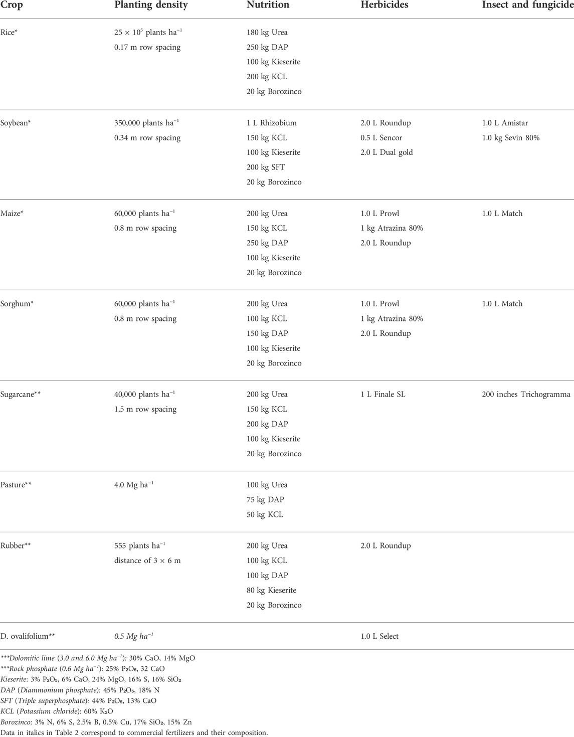
TABLE 2. Fertilization of the production systems according to requirements.
2.2 Statistical design
The statistical design was a completely randomized block design on a split-split plot arrangement of treatments with four replicates with production systems ACR-S, ACR-MS, SM, R-Do, PBd-ACR and NS as control as the main plot, doses of dolomitic lime (3.0 and 6.0 ton ha−1) as subplots and tillage systems (chisel, harrow, and mouldboard) as sub-subplots. Each experimental unit comprised 400 m2 (20 m × 20 m).
2.3 Soil fertility and water provision ecosystem services
Soil chemical and physical properties were determined once every year to estimate indicators related to soil fertility and water provision. The organic matter content, the exchangeable bases such as calcium (Ca), magnesium (Mg), potassium (K), exchangeable acidity as aluminum (Al), and pH were determined from each experimental plot at four depths (0–10, 10–20, 20–30, 30–40 cm). The analytical methods used to determine soil chemistry variables are described in Table 3.
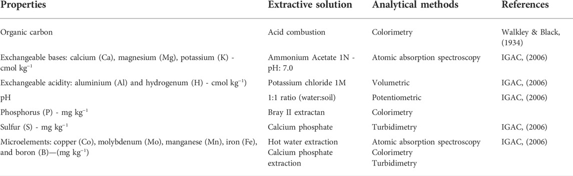
TABLE 3. Analytical methods used for the determination of soil chemistry properties.
Soil physical properties associated with the water provision indicator were taken at four depths (0–10; 10–20; 20–30, and 30–40 cm) in each experimental unit and are described in Table 4.
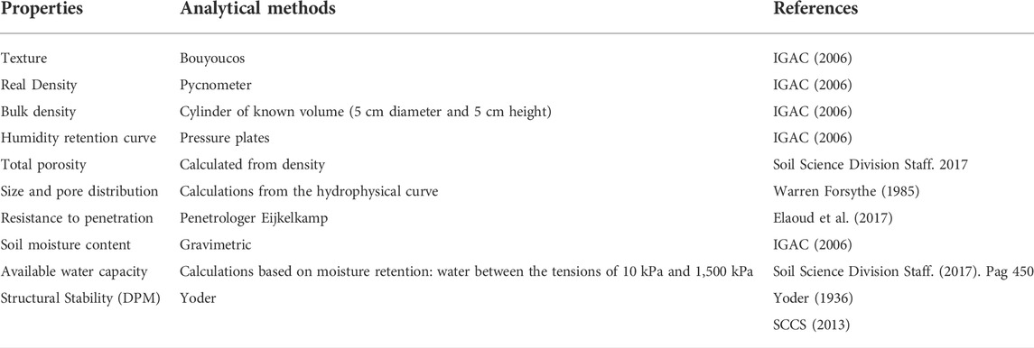
TABLE 4. Analytical methods used for the determination of soil physical properties.
2.4 Soil diversity ecosystem services
2.4.1. Soil macroinvertebrates
The number of edaphic macroinvertebrates was determined once every year using The Tropical Soil Biology and Fertility (TSBF) method (Anderson and Ingram, 1993). A 25 × 25 × 20 cm block of soil at three random points in each experimental plot was sampled. Organisms were separated manually; morphotypes were preserved with 70% alcohol and, with earthworms, 4% formalin. Counting and identification down to the order level were made by observation using a stereomicroscope. Taxonomic richness, abundance, and Simpson diversity index were calculated. The morphospecies accumulation curve was determined using the EstimateS program (Version 9.1.0, Copyright RK Colwell: http://purl.oclc.org/estimates).
2.5 Soil greenhouse gas fluxes and carbon storage
GHG sampling was conducted after implementing agricultural practices, mainly fertilization and tillage. From 2012 to 2015, monthly samples were taken in ACR-MS, SM, PBd-ACR and NS systems to determine the fluxes of nitrous oxide (N2O), carbon dioxide (CO2), and methane (CH4) emitted by the soil. The samples were taken from closed chambers installed in each production system at 5 cm depth. Sample analysis was performed in a Shimadzu GC-14A gas chromatograph, equipped with ECD (electron capture detector for N2O) and FID (flame ionization detector for CH4) detectors. A gas analyzer (Qubit Systems S151 with IRGA infrared technology) was used for CO2.
The fluxes were calculated following the GRACEnet method (Parkin and Venterea, 2010). The results were reported as the concentration in ppm (v/v) and were transformed into mass units according to the ideal gas Equation 1:
Where:
P: Atmospheric pressure of the area under study (0.97 atm).
V: Volume (L).
n: Number of moles.
R: Ideal gas constant (0,08206 L atm mol−1 K−1).
T: Temperature inside the chambers in K.
GHG fluxes were estimated by non-linear (Hutchinson and Mosier, 1981) and linear regression using the HMR library (version 0.4.1) of R (Pedersen et al., 2010). Due to the high sensitivity of non-linear fluxes in changes of concentration, those that met the 5% rejection criterion of the null hypothesis of fluxes equal to zero (H0) were determined as significant. Otherwise, fluxes estimated with a linear regression that met at least 30% probability of rejection of H0 were used.
Soil organic matter and bulk density (BD) values at two depths (0–10 and 10–20 cm) were used to estimate each experimental unit’s soil organic carbon storage.
2.6 Statistical analysis
2.6.1 Soil ecosystem indicator calculation
Principal Component Analysis (PCA) was used to identify the chemical, physical and biological (soil macroinvertebrates) variables that best discriminate the difference between the system´s productivity at two depths (0–10 and 10–20 cm). And from there, the ecosystem services (ES) indicators of fertility, water regulation, and biodiversity were generated. For the construction of the indicator, variables with positive or negative contributions were selected according to the correlation circle (>50% of the maximum value, to components 1 and 2). The variable’s value is multiplied by the corresponding weight factor for each variable. The indicator values were calculated according to Equation 2 proposed by Velasquez et al. (2007):
Ii1: the value of ecosystem services indicator i in experimental sampling plot 1.
F1 and F2: % of the variance value explained by principal components 1 and 2 estimated from PCA of the data set of indicators Ii
αI, βI, γI: respective contributions of variables a, b, and c corresponding to components 1(I) and 2 (II).
a, b, c = values of the variables measured in experimental unit 1
Values were transformed to a range between 0.1 and 1.0, where 1 represents the maximum value for the ecosystem services measured in each system (Rodriguez et al., 2013). The ADE 4 1.4.5 library (Dray and Dufour, 2007) of the R program (R Core Team, 2019) was used for the calculation.
The GHG-based climate regulation indicator was estimated from cumulative emissions of CO2 equivalent and carbon stock by transforming the values between 0.1 and 1 (Lavelle et al., 2014). Carbon stock was calculated from the soil organic carbon (SOC) concentration multiplied by the bulk density (BD) at depth (0–10 and 10–20 cm).
Indicators associated with the production systems were compared using ANOVA (p ≤ 0.05), and the comparison test between means was performed by applying LSMeans with α = 0.05 significance level with the statistical program SAS (Inst. Inc.) version 9.0.
3 Results
3.1 Soil fertility indicator
Principal Component Analysis showed that Ca, Mg, Al, and pH at the 0–10 and 10–20 cm depths were variables with the highest influence on components 1 and 2 during the study period. These variables were used to calculate the fertility indicator in 2011. For 2012, 2013, and 2014, the variables Cu, Mo, S, P, and Mn were added to Ca, Mg, Al and pH, for the PCA (see Supplementary Material SB and SC). The NS value for 2011, was 0.11 and it was considered the reference point to determine the effect of soil management change. After the soil intervention for the establishment of crops, the fertility indicator reached a value of 0.39 (p ≤ 0.05) in the ACR-S and ACR-MS, in 2011. PBd-ACR and R-Do showed the highest values, with indicators of 0.47 and 0.44, respectively, without statistically significant differences from the other crops established in 2012. No statistically significant differences were evidenced for the soil fertility indicator in all production systems in 2013 and 2014. However, PBd-ACR and R-Do showed higher values, indicating increases over native savanna of 70% (Table 5).
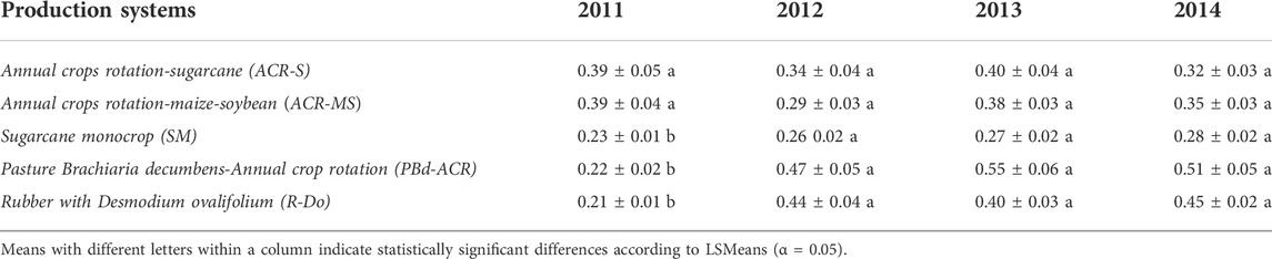
TABLE 5. Soil fertility indicator valued in production systems established in an Oxisol of the Meta High Plains.
In evaluating the fertility indicator in the production systems and the effect of incorporating 3.0 and 6.0 ton ha−1 of lime, no statistically significant differences were found between the doses applied to the soil in 2011. For 2013 and 2014, a higher Ca availability was found in the soil with 6.0 ton ha−1 (2.5–3.2 cmol kg−1), while the limed soil with 3.0 ton ha−1 presented a Ca concentration between 1.3 and 1.8 cmol kg−1.
3.2 Soil water function indicator
Principal Component Analysis indicated that bulk density (BD) and pore distribution at the macropore, mesopore, and micropore levels contributed more than other variables to components 1 and 2 during the sampling period (see supplementary material D and E); BD presented the greatest weight for component 1, at depths of 0–10 cm. Water function indicators were calculated and associated with soil moisture storage capacity and porosity. The indicator value for the NS was 0.32, considering that no mechanical soil removal was performed. The values found in production systems ranged between 0.30 and 0.67, which shows how the introduction of the crops affected these Oxisols. PBd-ACR and R-Do systems showed the greatest values during the evaluation period with 0.56 and 0.60, respectively, except in the fourth year, when the highest value was found in SM (0.67) (p ≤ 0.05) (Table 6).
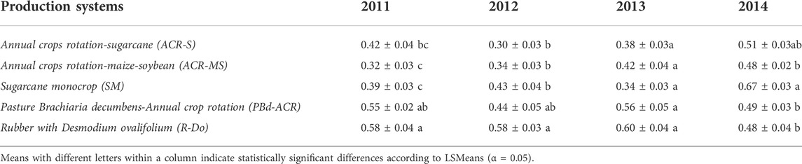
TABLE 6. Water provision indicator valued in the production systems established in an Oxisol of the Meta High Plains.
Soil BD for the NS was 1.6 g cm−3 in 2011. After soil preparation, the values were between 1.17 and 1.40 g cm−3 in the first 10 cm of depth for production systems. The R-Do and PBd-ACR systems had low values of 1.35 and 1.40 g cm−3 respectively, at a depth of 0–10 cm. ACR-S and SM decreased BD for 2014. The water regulation indicator was higher in production systems with lower BD, showing an inverse relationship.
3.3 Soil diversity indicator
The analysis identified 16 orders of macroinvertebrates. PCA showed that abundance (measured as population density or individuals per square meter), Blattodea, Hymenoptera, and Coleoptera were the highest contributing variables in components 1 and 2 during the sampling period (see supplementary material F and G).
The biodiversity indicator of the native savanna taken as a reference in 2011 was 0.79. This value was statistically and significantly different from values for ACR-S (0.28), ACR-MS (0.24), SM (0.27), PBd-ACR (0.30), and R-Do (Table 7). For 2012 and 2013, an increase in the biodiversity indicator was observed in the ACR-S, ACR-MS, SM and R-Do systems. The difference could be related to soil and crop management practices that favored the density of edaphic macrofauna. In general, all the production systems except PBd-ACR showed an increase in the biodiversity indicator throughout the evaluation period compared to the NS whose value decreased in 2014 (0.55).
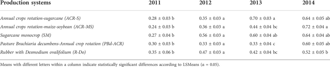
TABLE 7. Soil diversity indicator valued in the production systems established in an Oxisol of the Meta High Plains.
In 2011, termites were the most abundant group at depths of 0–10 cm of soil, followed by beetles and ants with densities of 6,981, 1,581, and 1,300 individuals per meter squared, respectively. Earthworms were found in lower abundance with a density of 263. At 10–20 cm of soil depth, there was a 34% decrease in the abundance of termites (2,344 individuals per meter squared) and 69% for beetles (1,088 individuals per meter squared). Termite abundance reached densities of 4,213, 1,556, and 1,858 after conversion from NS to R-Do and PBd-ACR, the highest abundance of termites was obtained after the NS without intervention with densities of 4,213, 1,556, and 1,858 individuals per meter squared, respectively or 2012, 2013, and 2014. For R-Do, SM and ACR-S there was a higher abundance of termites, ants, and beetles than the abundance of earthworms, which were lower in all systems every year evaluated.
3.4 Carbon stock indicator
The analysis gave a 2011 reference value of 0.40 for the carbon stock indicator in NS at a depth of 0–20 cm. No statistically significant differences were observed between production systems and the carbon stock indicator during the evaluation period (Table 8). After plowing and lime fertilization, carbon stock indicators for harrow and mouldboard tillage were statistically different, with values of 0.49 and 0.41, respectively, according to the analysis of variance after the first year (Table 9). In 2012, the same pattern of the previous year was maintained, with differences detected only for tillage, with a decrease of almost one point with respect to the last year, with values of 0.35 for harrow tillage and 0.31 for mouldboard tillage. However, the significance slightly exceeded 5%. In 2013 and 2014, the analysis showed no statistically significant effects for the applied treatments. The indicator values for these years are similar to those obtained in 2012 (see supplementary material H).
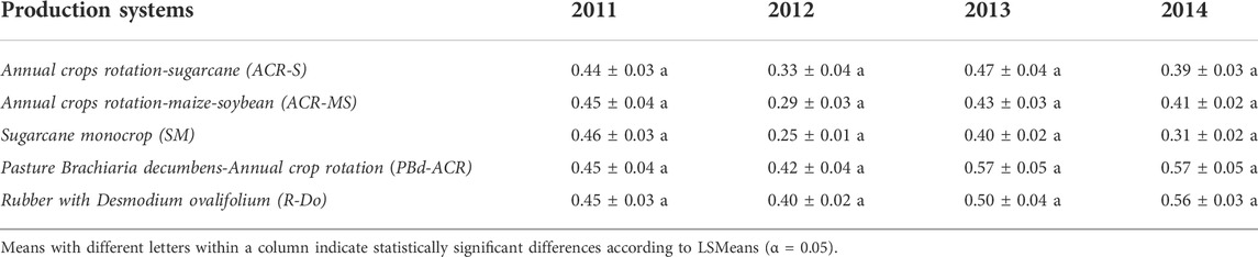
TABLE 8. Stock carbon indicator valued in the production systems established in an Oxisol of the Meta High Plains.

TABLE 9. Stock carbon indicator valued with tillage implement in an Oxisol of the Meta High Plains.
3.5 Greenhouse gas emission indicator
For the construction of the GHG indicator, soil emissions measured for CO2, N2O, and CH4 were integrated to express them as CO2 equivalent in Mg ha−1 year−1. In 2011, measurements were made in the last months, when the management of the systems was established, and GHG was only measured in a fraction of the year. This period was excluded from the indicator analysis. In all systems, the indicator value was lower than 0.5, except for the SM system, which in 2014 presented a value of 0.60. The ACR-MS system did not show significant differences over the years; despite having agronomic management, the values obtained are close to the savanna, whose reference value in 2012 was 0.30. The low values of the indicator were qualified as positive because they were related to lower GHG emissions (Table 10).

TABLE 10. GHG indicator valued in the productive systems established in an Oxisol of the Meta High Plains.
The analysis of nitrous oxide emissions for 2012 did not present differences for tillage implements, systems, and lime doses or their interactions; the range was defined between the SM system with 0.47 g ha−1 day−1 and the ACR-MS system with 0.94 g ha−1 day−1. In 2013, the highest N2O emission values of the years evaluated were evidenced, ranging between 2.5 g ha−1 day−1 for the SM system to 4.6 g ha−1 day−1 for the PBd-ACR and ACR-MS systems. N2O emissions decreased for the systems reported above. In the case of the native savanna, emissions were close to those reported for the SM system, with the lowest values during the evaluation period.
Statistically significant differences were observed with respect to carbon dioxide for the production systems factor for all the years evaluated. The PBd-ACR and ACR-MS systems presented the highest values, with averages of 4.0 kg ha−1 day−1. The NS presented similar values to ACR-MS, showing the lowest emissions with 3.1 and 2.5 kg ha−1 day−1, respectively. The highest CO2 emissions were found in 2014, when the SM production system showed a value of 7.4 kg ha−1 day−1 and PBd-ACR was 6.7 kg ha−1 day−1. In the NS the emission value for the same period was 6.0 kg ha−1 day−1. The SM system was the only one where methane emissions were detected, with a range for the years evaluated between 0.20 g ha−1 day−1 and 0.97 g ha−1 day−1. In the native savanna as a control, no statistically significant emissions were detected for this gas (see supplementary material I).
4 Discussion
Oxisols are generally of low fertility, with high acidity and poor content of exchangeable bases such as Ca and Mg. These conditions limit agricultural production, making it necessary to establish production systems based on tillage and fertilizers, contributing to more productive topsoil (Amezquita et al., 2004). This research showed significant changes in soil fertility when NS are converted to production systems with correctives and fertilizers, increasing the concentration of Ca, Mg, pH, and decreasing Al in the soil. The fertility indicator synthesized from the analysis of these variables was sensitive and only allowed discrimination of these changes between production systems for 2011. These changes in the fertility indicator were also observed in a study conducted by Lavelle et al. (2014), in farmers’ fields in the Meta High Plains, and allowed differentiating the agronomic management applied between transient crop systems, pastures and permanent crops, such as rubber and oil palm. NS conversion to production systems, using 3.0 and 6.0 Mg ha−1 of lime incorporated with tillage implements, had a positive effect on the correction of soil acidity, increasing the pH to values above 5.5 in the first 20 cm of depth. Gallo et al. (2013) reported similar results showing that Ca and Mg concentrations in a High Plains Oxisol were higher at depths 0–10 y 10–20 cm. Incorporating correctives in Oxisols is a common practice to reduce Al levels and increase the contents of exchangeable bases in the soil (Sánchez et al., 1991). According to Amezquita (1999), the tillage implements for incorporating lime at greater depths in the soil profile and the establishment of crops that provide deep roots are strategies that lead to improving the productivity and persistence of production systems in the Colombian High Plains.
Analysis of physical properties revealed differences in the change in soil use and between the systems established for 2011. The indicator’s value also increased in the following years, with the SM system, regardless of the application of lime and tillage, presenting the highest value. This effect can be explained because of sugarcane´s characteristic as a deep-rooted crop. Sugarcane´s deep roots result from long growth cycles and longevity of the root system through periodic harvests, where the ratoon resprouts and remains in the soil over time (Venu et al., 2017).
Regarding soil physical variables and the changes derived from converting NS, practices implemented in 2011 had an impact in the first 20 cm of depth, with significant changes in the hydrophysical properties. Macropore and mesopore percentage increased in the first year. Subsequently, they decreased in a differentiated manner among the SM systems. ACR-MS and PBd-ACR systems were established, with mechanized soil tillage necessary for the establishment of crops in 2014. Critical levels identified for mechanization decisions were percentages of macropores less than 10%, mesopores less than 8% and micropores greater than 30%, and a bulk density greater than 1.6 g cm−3 in the first 20 cm of depth. Baquero and Rojas (2001) and Baquero et al. (2001) showed that the Oxisols of the High Plains are highly resilient. The effects of tillage on some physical properties are temporary, requiring contributions of organic carbon for those effects to be stable for more extended periods, consolidating the porous structure achieved and decreasing the frequency of mechanization.
The biodiversity indicator showed substantial differences among production systems established in 2011, 2012 and 2013 compared to the NS. Biodiversity increased in the SM system from the year 2012, a result that can be associated with the soil’s physical variables, where there was a greater presence of macropores and mesopores. Earthworms (Haplotaxia) were the organisms with the lowest abundance throughout the evaluation period. This result may be associated with the effect of soil management during the establishment and maintenance of the built production systems. The same tendency of the indicator was seen in the systems whose management was reduced, such as ACR-S and SM. The biodiversity indicator was lower during 2012 and 2013 in ACR-MS and PBd-ACR. The evaluation of soil macroinvertebrates showed that the highest abundance occurred in the first 10 cm of depth. Sixteen taxonomic orders were identified, where the highest abundance was related to the Blattodea (termites), Hymenoptera (ants), and Coleoptera (beetles). Similar results were obtained by Pérez et al. (2019) in an Oxisol of the Colombian High Plains under different pasture management, where the order Blattodea presented the greatest densities, representing 72% of the total abundance found in the soil. According to Jiménez et al. (2006), termites and earthworms are the dominant edaphic macrofauna in tropical savannas, such as the Brazilian Cerrado and the Eastern Plains of Colombia. Jouquet et al. (2016) indicated that the edaphic macrofauna represents an important biological component of tropical soils and is related to the soil’s physical properties, such as porosity and density. For example, through their activity as soil engineers, termites can contribute to the maintenance of aeration, water infiltration, and climate control through carbon conservation.
Bulk density (BD) and soil organic carbon content, as independent variables, showed differences among production systems when both were analyzed for 0–10 cm and 10–20 cm depth. However, the analysis of variance for the indicator associated with carbon content from 0 to 20 cm depth, calculated based on those two variables, showed a significant effect due to the tillage implements used for soil conditioning, but did not show significant differences between production systems over time. Similar results were reported by Hati et al. (2007) for these same variables, BD and SOC. In addition, these authors found that SOC has beneficial effects on soil physical properties with reduced BD and increased microorganism activity.
The results for GHGs showed that production systems emissions were related to precipitation events, but not with tillage, lime dosage, and their interaction. During the emissions evaluation period, the highest CO2 emissions were reported in 2013, the year with the highest rainfall with an average of 2,170 mm. Sugarcane was the crop with the highest methane. The agronomic management of the SM that remained throughout the years of evaluation had a variation compared to the other systems. It involved the cutting of stems, regrowth of plant material, and crop residues, combined with periodic fertilization. Compared to the other systems, this differential management may have contributed to the higher methane and nitrous oxide emissions, related to the higher amount of organic carbon in the soil and the abundance of termites.
4.1 Integration of indicators
The construction and analysis of the fertility, water regulation, climate regulation (SOC and GHG), and biodiversity indicators, allows comparison of production systems and guidance for land-use change strategies. Benefits should be identified for at least one ecosystem services as compared to the native savanna, even though the provision of other services may decrease over time. Thus, for soil fertility, conversion of NS increased the indicator for two production systems, PBd-ACR and R-Do. For the other three systems, the impact was lower. These results are similar to those obtained by Lavelle et at., (2014) where they indicated that annual crops have a positive impact on these Oxisol´s fertility indicator.
Nutrient supply is improved by incorporating fertilizers, but those negatively impact macroinvertebrate communities affecting the biodiversity indicator. In contrast with the biodiversity indicator, the water regulation and soil carbon indicators showed improved physical conditions of soil in the evaluated systems. Sustainable soil use requires the analysis of tradeoffs that allow for a balance between supply and demand of ES, thus favoring ecosystem functions and their long-term maintenance.
5 Conclusion
The evaluated indicators made it possible to identify the positive and negative effects of converting native savanna to agricultural production systems. The PBd-ACR systems raised soil fertility. Converting NS negatively affects climate control indicators, especially GHG emissions; for the carbon stock, the impact is not so clear. The carbon stock indicator did not help to differentiate impacts of converting Oxisol savannas to the proposed systems. Decreases in topsoil bulk density due to conversion and soil conditioning may have complicated the evaluation of carbon.
The strategy of incorporating corrective measures and deep tillage positively affected some ES indicators provided by Oxisols of the Colombian Eastern High Plains for the first 3 years. However, from the fourth year of soil use change, fertility and water functions decreased, showing the need to carry out conditioning again to maintain soil characteristics required for productive sustainability.
This research showed that the use of deep tillage to incorporate long-term amendments for production systems is an alternative for the management of Oxisols. Deep tillage can reduce the frequency of mechanical alteration needed for the system, which is traditionally done at each planting or crop renewal period.
Periodic monitoring of ES indicators made it possible to identify how land-use change and tillage management practices and the application of correctives positively or negatively affect some soil properties. The selection of variables with the greatest contribution to the construction of ES indicators allows for reducing the number of measurements required to make management decisions at the local level to maintain and conserve the balance of production systems.
Data availability statement
The datasets presented in this article are readily available. The data generated in this research may be shared once Agrosavia and the intellectual property department authorize it. Requests to access the datasets should be directed to propiedadintelectual@agrosavia.co.
Author contributions
JEB and JHBR developed and managed the research project. JEB, JHBR, OGG, and JOA participated in the planning of field trials and the consolidation of experimental data. MA performed a statistical analysis of the data. LMMC and NSRH prepared the manuscript with important contributions from all authors.
Funding
This research was financed by the Colombian Ministry of Agriculture and Rural Development (MADR) through a special technical and scientific cooperation agreement 1726 between the Colombian Research Corporation -Agrosavia and the International Center for Tropical Agriculture (CIAT).
Acknowledgments
The authors would like to thank the Colombian Ministry of Agriculture and Rural Development for financing this research; the researchers and operators of the International Center for Tropical Agriculture (CIAT) who participated in the execution of activities and field sampling, as well as the support professionals and operators of the Colombian Agricultural Research Corporation Agrosavia for their follow-up and support in data collection.
Conflict of interest
The authors declare that the research was conducted in the absence of any commercial or financial relationships that could be construed as a potential conflict of interest.
Publisher’s note
All claims expressed in this article are solely those of the authors and do not necessarily represent those of their affiliated organizations, or those of the publisher, the editors and the reviewers. Any product that may be evaluated in this article, or claim that may be made by its manufacturer, is not guaranteed or endorsed by the publisher.
Supplementary material
The Supplementary Material for this article can be found online at: https://www.frontiersin.org/articles/10.3389/fenvs.2022.687804/full#supplementary-material
References
Alexander, P., Rounsevell, M. D. A., Dislich, C., Dodson, J. R., Engstrom, K., and Moran, D. (2015). Drivers for global agricultural land use change: The nexus of diet, population, yield and bioenergy. Glob. Environ. Change 35, 138–147. doi:10.1016/j.gloenvcha.2015.08.011
Amezquita, E. (1999). Physical properties of the Llanos Orientales soils and their requirements of tillage. Palmas 20 (1), 73–86. Available at: https://publicaciones.fedepalma.org/index.php/palmas/article/view/692.
Amézquita, E., Rao, I. M., Rivera, M., Corrales, I., and Bernal, J. H. (2013). Sistemas agropastoriles: Un enfoque integrado para el manejo sostenible de Oxisoles de los Llanos Orientales de Colombia. Centro Internacional de Agricultura Tropical (CIAT)-Ministerio de Agricultura y Desarrollo Rural (MADR) de Colombia; Corporación Colombiana de Investigación Agropecuaria (Corpoica). 288 p. (Documento de Trabajo CIAT No. 223). ISBN 978-958-694-117-4. Available at: http://ciatlibrary.ciat.cgiar.org/Articulos_Ciat/biblioteca/Sistemas_Agropastoriles.pdf#page=247.
Amezquita, E., Thomas, R. J., Rao, I. M., Molina, D. L., and Hoyos, P. (2004). Use of deep-rooted tropical pastures to build-up an arable layer through improved soil properties of an Oxisol in the Eastern Plains (Llanos Orientales) of Colombia. Agric. Ecosyst. Environ. 103, 269–277. doi:10.1016/j.agee.2003.12.017
Anderson, J. M., and Ingram, J. S. I. (1993). Tropical soil Biology and fertility programe. A handbook of methods. Available at: http://courses.washington.edu/esrm304a/lectures/Soils/Tropical%20Soil%20Biology%20and%20Fertility%20Methods_Web%20Soils%20Reading.pdf.
Baquero, J. E., and Rojas, L. A. (2001). “Interaction effects of organic materials and lime on grain yield and nutrient acquisition of three maize varieties grownin an Oxisol of the Colombia Eastern Plains,” in Plant Nutrition – food security and sustainability of agroecosystems. Editors W. J. Horst, and M. K. Schenk (Printed in Netherlands: Published by Kluwer Academic Publishers). ISBN 0-7923-7105-4: 982-983.
Baquero, J. E., Aristizábal, Q. D., Rendón, W., and Salamanca, C. R. (2001). Manejo conservacionista de los suelos arroceros de la Orinoquia Colombiana. Boletín técnico N° 32. Corpoica- Pronatta. Edit. JARAMILLO, C. 60 p. ISBN 958-33-5894-0. Available at: http://hdl.handle.net/11348/6714.
Bernal, J. H., Peña, A. J., Díaz, N. C., and Obando, D. (2013). Condiciones Climáticas de la Altillanura Plana Colombiana en el Contexto de Cambio Climático. En: Sistemas Agropastoriles: Un Enfoque Integrado para el Manejo Sostenible de Oxisoles de los Llanos Orientales de Colombia. ISBN 978-958-694-117-4. Available at: http://ciat-library.ciat.cgiar.org/articulos_ciat/biblioteca/Sistemas_Agropastoriles.pdf#page=28.
Costanza, R. (2016). “Ecosystem services in theory and practice,” in Handbook of ecosystem services. Editors M. Potschin, R. Haines- Young, R. U. Fish, and R. K. Turner (London and New York: Routledge). eBook ISBN 9781315775302.
de Espindola, G., de Silva Figueredo, E., Picanço, P., and dos Reis, A. (2021). Cropland expansion as a driver of land-use change: The case of cerrado-caatinga transition zone in Brazil. Environ. Dev. Sustain. 23, 17146–17160. doi:10.1007/s10668-021-01387-z
de Vries, F., Thébaultc, E., Liiri, M., Birkhofer, K., Tsiafouli, M., Bjørnlund, L., et al. (2013). Soil food web properties explain ecosystem services across European land use systems. Proc. Natl. Acad. Sci. U. S. A. 110 (35), 14296–14301. doi:10.1073/pnas.1305198110
Deng, X., Li, Z., Huang, J., Shi, Q., and Li, Y. (2013). A revisit to the impacts of land use changes on the human wellbeing via altering the ecosystem provisioning services. Adv. Meteorology 8, 907367. doi:10.1155/2013/907367
Soil Science Division Staff (2017). “Soil survey manual,” in USDA handbook 18. Editors C. Ditzler, K. Scheffe, and H. C. Monger (Washington, D.C: Government Printing Office).
Dray, S., and Dufour, A.-B. (2007). The ade4 package: Implementing the duality diagram for ecologists. J. Stat. Softw. 22 (4), 1–20. doi:10.18637/jss.v022.i04
Duru, M., Therond, O., Martin, G., Martin-Clouaire, R., Magne, M. A., Justes, E., et al. (2015). How to implement biodiversity-based agriculture to enhance ecosystem services: A review. Agron. Sustain. Dev. 35, 1259–1281. doi:10.1007/s13593-015-0306-1
Elaoud, A., Hassen, H. B., Salah, N. B., Masmoudi, A., and Chehaibi, S. (2017). Modeling of soil penetration resistance using multiple linear regression (MLR). Arab. J. Geosci. 10, 442. doi:10.1007/s12517-017-3235-2
Foley, J. A., DeFries, R., Asner, G. P., Barford, C., Bonan, G., Carpenter, S. R., et al. (2005). Global consequences of land use. Science 309 (5734), 570–574. doi:10.1126/science.1111772
Forsythe, W. (1985). Física de Suelos. Manual de laboratorio. la Ed. San José, Ipis, Costa Rica: IICA, San José de Costa Rica, 211p.
Fu, B., Li, Y., Wang, Y., Zhang, B., Yin, S., Zhu, H., et al. (2016). Evaluation of ecosystem service value of riparian zone using land use data from 1986 to 2012. Ecol. Indic. 69, 873–881. doi:10.1016/j.ecolind.2016.05.048
Fu, Q., Li, B., Hou, Y., Bi, X., and Zhang, X. (2017). Effects of land use and climate change on ecosystem services in central asia's arid regions: A case study in altay prefecture, China. Sci. Total Environ. 607-608, 633–646. doi:10.1016/j.scitotenv.2017.06.241
Gallo, O., Bernal, J., Baquero, J. E., Botero, R., and Gómez, J. (2013). Efecto de tres métodos de incorporación de cal dolomítica en la altillanura plana colombiana. Suelos Ecuat. 43 (1), 24–28. ISSN 0562-5351. Available at: http://www.unicauca.edu.co/revistas/index.php/suelos_ecuatoriales/article/view/52.
Hasan, S. S., Zhen, L., Miah, G., Ahamed, T., and Samie, A. (2020). Impact of land use change on ecosystem services: A review. Environ. Dev. 34, 100527. doi:10.1016/j.envdev.2020.100527
Hati, K. M., Swarup, A., Dwivedi, A. K., Misra, A. K., and Bandyopadhyay, K. K. (2007). Changes in soil physical properties and organic carbon status at the topsoil horizon of a vertisol of central India after 28 years of continuous cropping, fertilization, and manuring. Agric. Ecosyst. Environ. 119, 127–134. doi:10.1016/j.agee.2006.06.017
Huertas, H., Rangel, J., and Parra, A. (2018). Caracterización de la fertilidad química de los suelos en sistemas productivos de la altillanura plana, Meta, Colombia. luaz. 46, 54–69. doi:10.17151/luaz.2018.46.5
Hutchinson, G. L., and Mosier, A. R. (1981). Improved soil cover method for field measurement of nitrous oxide fluxes. Soil Sci. Soc. Am. J. 45, 311–316. doi:10.2136/sssaj1981.03615995004500020017x
IGAC - Instituto Geográfico Agustín Codazzi (2002). Atlas de Colombia. 5.a ed. Bogotá, Colombia: IGAC.
IGAC - Instituto Geográfico Agustín Codazzi (2006). Métodos analíticos del laboratorio de suelos 6 edición. Bogotá, Colombia: IGAC.
Jiménez, J., Decaëns, T., and Lavelle, P. (2006). Nutrient spatial variability in biogenic structures of Nasutitermes (Termitinae; Isoptera) in a gallery forest of the Colombian "Llanos. Soil Biol. Biochem. 38 (5), 1132–1138. doi:10.1016/j.soilbio.2005.09.026
Jouquet, P., Bottinelli, N., Shanbhag, R. R., Bourguignon, T., Traoré, S., and Shahid Abbas Abbasi, S. A. (2016). Termites: The neglected soil engineers of tropical soils. Soil Sci. 181, 157–165. doi:10.1097/SS.0000000000000119
Kertész, Á., Nagy, L. A., and Balázs, B. (2019). Effect of land use change on ecosystem services in Lake Balaton Catchment. Land Use Policy 80, 430–438. doi:10.1016/j.landusepol.2018.04.005
Kertész, Á. (2017). “The effect of land degradation on ecosystem services,” in Ecosystem services of headwater catchments. Editors J. Křeček, M. Haigh, T. Hofer, E. Kubin, and C. Promper (New Delhi: Springer India), 209–216. doi:10.1007/978-3-319-57946-7_18
Klink, C., and Machado, R. (2005). Conservation of the Brazilian Cerrado. Conserv. Biol. 19 (3), 707–713. doi:10.1111/j.1523-1739.2005.00702.x
Lavelle, P., Rodríguez, N., Arguello, O., Bernal, J., Botero, C., Chaparro, P., et al. (2014). Soil ecosystem services and land use in the rapidly changing Orinoco River Basin of Colombia. Agric. Ecosyst. Environ. 185, 106–117. doi:10.1016/j.agee.2013.12.020
Lawler, J. J., Lewis, D. J., Nelson, E., Plantinga, A. J., Polasky, S., Withey, J. C., et al. (2014). Projected land-use change impacts on ecosystem services in the United States. Proc. Natl. Acad. Sci. U. S. A. 111 (20), 7492–7497. doi:10.1073/pnas.1405557111
Lorz, C., Neumann, C., Bakker, F., Pietzsch, K., Weiss, H., and Makeschin, F. (2012). A web-based planning support tool for sediment management in a meso-scale river basin in Western Central Brazil. J. Environ. Manage. 127, S15–S23. doi:10.1016/j.jenvman.2012.11.005
Millennium Ecosystem Assessment (2005). Ecosystems and human well-being: Synthesis. Washington, DC: Island Press. Available at: www.millenniumassessment.org.
Parkin, T. B., and Venterea, A. (2010). Chapter 3. Chamber-base trace gas flux measurements. Follett RF Sampl. Protoc. 3, 1–39.
Pedersen, A. R., Petersen, S., and Scheldeb, K. (2010). A comprehensive approach to soil-atmosphere trace-gas flux estimation with static chambers. Eur. J. Soil Sci. 61, 888–902. doi:10.1111/j.1365-2389.2010.01291.x
Pereira, P., Bogunovic, I., Muñoz-Rojas, M., and Brevik, E. (2018). Soil ecosystem services, sustainability, valuation, and management. Current Opinion in. Environ. Sci. Health 5, 7–13. doi:10.1016/j.coesh.2017.12.003
Pérez-López, O., Bueno, G. A., Baquero, J. E., Onofre, H. G., Cassalett-Bustillo, E., Molina, A. M., et al. (2019). Modelo productivo tecnologías integrales para sistemas de producción de bovinos de cría en la altillanura colombiana. Mosquera, Colombia: Corporación Colombiana de Investigación Agropecuaria (AGROSAVIA). ISBN E book: 978-958-740-268-1.
R Core Team (2019). R: A language and environment for statistical computing. Vienna, Austria: R Core Team. Available at: http://www.r-project.org/.
Rivas, L., Hoyos, P., Amézquita, E., and Molina, D. L. (2004). “Manejo y uso de los suelos de la Altillanura Colombiana,” in En Centro Internacional de Agricultura Tropical (CIAT) (Eds.), Manejo y uso de los suelos de la Altillanura Colombiana. Análisis económico de una estrategia para su conservación y mejoramiento. Construcción de la capa arable (Cali, Colombia: CIAT), 6–12. Available at: http://ciat-library.ciat.cgiar.org/Articulos_Ciat/degradacion_capa_arable.pdf.
Rivera, M., Amézquita, E., Rao, I. M., Corrales, I. I., and Chávez, L. F. (2013). “Establecimiento de sistemas agropastoriles y su efecto en el rendimiento de cultivos en suelos ácidos de sabanas,” in Sistemas agropastoriles: Un enfoque integrado para el manejo sostenible de Oxisoles de los llanos orientales de Colombia. Editors E. E. Amézquita, I. M. Rao, M. Rivera, I. Corrales, and J. H. Bernal (Cali, Colombia: Centro Internacional de Agricultura Tropical (CIAT); Ministerio de Agricultura y Desarrollo Rural (MADR) de Colombia; Corporación Colombiana de Investigación Agropecuaria (Corpoica)), 119–146. Available at: https://cgspace.cgiar.org/handle/10568/54575.
Rodríguez, A., Lavelle, P., Pulido, S. X., Gutierrez, A. J., Bernal, J., Arguello, O., et al. (2013). Construcción de indicadores de ecoeficiencia para la altillanura plana en los municipios de Puerto López y Puerto Gaitán, Departamento del Meta. ISBN 978-958-740-153-0. Available at: https://repository.agrosavia.co/bitstream/handle/20.500.12324/1868/60400_62674.pdf?sequence=1&isAllowed=y.
Rodríguez, B., Gonzalo, B. C., and Roger, A. (2019). Adopción e impacto de los sistemas agropecuarios introducidos en la altillanura plana del Meta. Cundinamarca, Colombia: Corporación Colombiana de Investigación Agropecuaria (Agrosavia). ISBN E-book: 978-958-740-296-4. doi:10.21930/agrosavia.analisis.7402964
Romero-Ruiz, M. H., Flantua, S. G. A., Tansey, K., and Berrio, J. C. (2012). Landscape transformations in savannas of northern South America: Land use/cover changes since 1987 in the Llanos Orientales of Colombia. Appl. Geogr. 32, 766–776. doi:10.1016/j.apgeog.2011.08.010
Sanchez, L. F., Baquero, J. E., and Munevar, F. (1991). Limitantes nutricionales para el establecimiento del cultivo de soya en Oxisoles de los Llanos Orientales. Suelos Ecuat. 21 (1), 5–16.
Sano, E., Rosa, R., Brito, J., and Ferreira, L. (2010). Land cover mapping of the tropical savanna region in Brazil. Environ. Monit. Assess. 166, 113–124. doi:10.1007/s10661-009-0988-4
SCCS - Sociedad Colombiana de la Ciencia del Suelo (2013). Ciencia del suelo: Principios básicos. - 2 edición burbano hernán y silva francisco. Dhaka, Bangladesh: SCCS.
Soil Survey Staff (2014). Keys to soil taxonomy. 12th ed. Washington, DC, USA: Soil Survey Staff. Available at: https://www.nrcs.usda.gov/wps/portal/nrcs/detail/soils/survey/class/taxonomy/?cid=nrcs142p2_053580.
Soil Survey Staff (1999). Soil taxonomy: A basic system of soil classification for making and interpreting soil surveys. 2nd ed. Washington, DC, USA: Soil Survey Staff. Available at: https://www.nrcs.usda.gov/Internet/FSE_DOCUMENTS/nrcs142p2_051232.pdf.
Thomas, R. J., and Ayarza, M. A. (1999). Sustainable land management for the oxisols of the Latin American savannas: Dynamics of soil organic matter and indicators of soil quality. Cali, Colombia: Centro Internacional de Agricultura Tropical (CIAT), 231. ISBN 958-694-011-X. Available at: https://cgspace.cgiar.org/bitstream/handle/10568/54288/Sustainable_land_management.pdf?sequence=1.
Tolessa, T., Senbeta, F., and Kidane, M. (2017). The impact of land use/land cover change on ecosystem services in the central highlands of Ethiopia. Ecosyst. Serv. 23, 47–54. doi:10.1016/j.ecoser.2016.11.010
Velasquez, E., Lavelle, P., and Andrade, M. (2007). GISQ, a multifunctional indicator of soil quality. Soil Biol. Biochem. 39 (12), 3066–3080. doi:10.1016/j.soilbio.2007.06.013
Venu, M. T., Madhu Bindu, G. S., Vijay Kumar, M., and Syamraj Naik, C. (2017). Study on root characteristics of sugarcane (saccharum officinarum) genotypes for moisture stress. Int. J. Plant Soil Sci. 18 (5), 1–4. doi:10.9734/ijpss/2017/34838
Walkley, A., and Black, I. A. (1934). An examination of the Degtjareff method for determining soil organic matter and a proposed modification of the chromic acid titration method. Soil Sci. 37 (1), 29–38. doi:10.1097/00010694-193401000-00003
Yoder, R. E. (1936). A direct meted of agregate analysis of soils and study of the physical nature of erosion losses. J. Am. Soc. Agron. 28, 337–351. doi:10.2134/agronj1936.00021962002800050001x(
Keywords: synthetic index, cos, GHG, native savanna, productive systems
Citation: Moreno-Conn LM, Rodríguez-Hernandez NS, Arguello JO, Gallo Gordillo O, Bernal-Riobo JH, Arango M and Baquero JE (2022) Land use change and its effect on ecosystem services in an Oxisol of the eastern High Plains of meta department in Colombia. Front. Environ. Sci. 10:687804. doi: 10.3389/fenvs.2022.687804
Received: 30 March 2021; Accepted: 11 October 2022;
Published: 25 October 2022.
Edited by:
Glenn Hyman, Self-employed, ColombiaReviewed by:
Jose Cora, São Paulo State University, BrazilPatrick Lavelle, Sorbonne Universités, France
Copyright © 2022 Moreno-Conn, Rodríguez-Hernandez, Arguello, Gallo Gordillo, Bernal-Riobo, Arango and Baquero. This is an open-access article distributed under the terms of the Creative Commons Attribution License (CC BY). The use, distribution or reproduction in other forums is permitted, provided the original author(s) and the copyright owner(s) are credited and that the original publication in this journal is cited, in accordance with accepted academic practice. No use, distribution or reproduction is permitted which does not comply with these terms.
*Correspondence: Lina M. Moreno-Conn, bG1vcmVub0BhZ3Jvc2F2aWEuY28=