 Cezar Morar1*†
 Tin Lukić2†
 Aleksandar Valjarević3†
 Liudmyla Niemets4†
 Sergiy Kostrikov4†
 Kateryna Sehida4†
 Ievegeniia Telebienieva4†
 Liudmyla Kliuchko4†
 Pavlo Kobylin4†
 Kateryna Kravchenko4†
- 1Department of Geography, Tourism and Territorial Planning, Faculty of Geography, Tourism and Sports, University of Oradea, Oradea, Romania
- 2Department of Geography, Tourism and Hotel Management, Faculty of Sciences, University of Novi Sad, Novi Sad, Serbia
- 3Department of Geospatial and Environmental Science, Faculty of Geography, University of Belgrade, Belgrade, Serbia
- 4Department of Human Geography and Regional Studies, Faculty of Geology, Geography, Recreation and Tourism, V.N. Karazin Kharkiv National University, Kharkiv, Ukraine
The contemporary globalized world characterizes the rapid population growth, its significant concentration in cities, and an increase in the urban population. Currently, many socio-cultural, economic, environmental, and other challenges are arising in modern cities, negatively affecting the state of the urban environment, health, and quality of life. There is a need to study these problems in order to solve them. Urban Green Areas (UGAs) are a part of the social space and a vital part of the urban landscape. They act as an environmental framework of the territory and a factor ensuring a more comfortable environment of human life. This study aims at substantiating the importance of the UGAs, identifying the spatiotemporal dynamics of their functioning, and transforming changes in their infrastructure given the expansion of their functions. This research was carried out as a case study of the second city in Ukraine, Kharkiv. The authors developed and used an original integrated approach using urban remote sensing (URS) and GIS for changes detection to evaluate the current state and monitor spatial transformations of the UGAs. We used several GIS platforms and online resources to overcome the lack of digital cadastre of the thematic municipal area of Kharkiv. This resulted in the present original study. The study analyses the dynamics of the spatial and functional organization of the UGAs according to the Master Plans, plans, maps, and functional zoning of the city for the period from 1867 to 2019. The peripheral green areas became important after the large-scale development of the extensive residential areas during the rapid industrial development in remote districts of the city. They provide opportunities for population recreation near living places. Central UGAs are modern, comprehensively developed clusters with multidisciplinary infrastructure, while the peripheral UGAs are currently being developed. The use of URS/GIS tools in the analysis of the satellite images covering 2000–2020 allowed identifying the factors of the UGAs losses in Kharkiv and finding that UGAs were not expanding and partially shrinking during the study period. It is caused by the intensive construction of the residential neighborhoods, primarily peripheral areas, infrastructure development, and expansion of the city transport network. Nonetheless, some sustainable trends of UGA functioning without more or less significant decrease could be proved as existing in a long-term perspective. The authors analyzed and evaluated changes and expansion of the UGAs functions according to modern social demand. The research value of this is the usage of different approaches, scientific sources, URS/GIS tools to determine the UGAs transformation in the second-largest city in Ukraine (Kharkiv), to expand and update the main functions of UGAs and their role in the population’s recreation. The obtained scientific results can be used to update the following strategies, programs, and development plans of Kharkiv.
1 Introduction
One of the most characteristic features of contemporary society is the rapid growth of cities and the continuously growing population rate, which leads to the intensification of information exchange and dynamic processes acceleration in the highly urbanized world. In this regard, residents of large cities suffer from emotional stress and fatigue, mainly due to increasing population density and many social problems and troubles. This fact leads to the increased demand for recreation, particularly for the green areas within the city, which are a necessary component of creating healthy, sustainable, and habitable cities, as highlighted in the report of the WHO Regional Office for Europe “Urban Green Space Interventions and Health” (WHO Regional Office for Europe, 2017a). The planning of cities worldwide is based on the sustainable development paradigm, enabling them to respond to the global environmental crisis by “greening.” The availability of urban greenery is considered key to urban sustainability progress in ecological, economic, and social terms (Du and Zhang, 2020). The availability of accessible and attractive green spaces is an integral part of the cities’ quality of life (Van Herzele and Wiedemann, 2003). UGAs are essential for the well-being of the population: the higher the people’s income, the larger the total area covered by green areas, the better the quality of these spaces, and the greater the number of private green areas (De la Barrera et al., 2016). As a component of urban greening or “green infrastructure,” UGAs are an important part of public open spaces and public services provided by cities that can serve as means of improving public health. They should be easily accessible to all population groups and fairly distributed within a city (WHO Regional Office for Europe, 2017b). Notoriously, UGAs are an integral part of the city’s structure. They affect the population’s living conditions by performing various sanitary, hygienic, and decorative planning functions. UGAs have a crucial role in ensuring the sustainability of the urban environment; they act as an environmental framework of the territory, a factor in providing a healthy (optimal) living environment, a place for recreational activities, and so forth. The supply level of the city’s population with green areas and their territorial distribution is an important task for local authorities and scientists to improve urban planning and strategic cities development.
It is commonly accepted that UGAs make a key performance in providing sustainability of the urban environment. Therefore, their distribution in a particular city and the relevant spatiotemporal dynamics should be a prime concern for municipalities. According to the information available from open sources, Ukraine lost almost 965,000 ha of its stand of trees only in 2001–2019, corresponding almost to 9% of the total national stand, if compared with the value in 2000. Although these values mainly concern the rural forest stand, this common trend obviously could not keep urban greening intact. Nonetheless, representative relevant research based on digital tools and technologies has not been accomplished for any urban territory in Ukraine yet.
A brief analysis of previous research demonstrates the considerable attention to studying the specific aspects of the green areas functioning. Much attention is paid to the study of certain aspects of sustainable urban development, including the planning structure of cities and the importance of recreational areas (Morar et al., 2016; Morar et al., 2019; Wolff and Haase, 2019; Snep et al., 2020; Morar et al., 2021a; Morar et al., 2021b; De Haas and Hassinkstuiver., 2021; Guenat et al., 2021; Rostang et al., 2021), implementation of the development strategies of Ukraine’s regions (Niemets K. et al., 2018), and regional development on the whole (Niemets et al., 2019c). In particular, Barrera et al. (2016) considered UGAs from the standpoint of the environmental framework of the territory. They evaluated the location planning and quality of UGAs based on the example of the Metropolitan Region of Santiago (Chile). They used such indicators in terms of the region as a whole and its municipalities as the total area of green zones per capita, quality of green areas. Garcia-Garcia et al. (2020) studied the problems of greenery planning in Madrid (Spain) during the twentieth century. The authors characterized three cases; described the preconditions of the urban project, planning evolution, and current situation; and compared the positions of UGAs. They developed quality index of urban green areas’ AMF, which is the sum of such blocks such as “accessibility,” “maintenance,” and “functionality.” Khoshtaria and Chachava (2017) considered the UGA as a basis for creating a favorable safe living situation, revealed the problem of greenery reduction and degradation in three resorts in southern Georgia, and assessed the protective role of greening from such natural disasters as torrential rains. Neuvonen et al. (2007) considered the recreational and tourist attractiveness of the UGA. They conducted a sociological survey on the recreation frequency in green areas, the types of human activities there, and the distance to green areas in Helsinki (Finland). Based on the example of Craiova city (Romania), Cianga and Popescu (2013) characterized the city’s parks, identified attractive green areas for tourists, and analyzed the characteristics of the green areas as tourist destinations and prospects for the tourist function development of green areas.
The application of methods and data of GIS, remote sensing, and spatial analysis for forest and UGAs changes was carried out by Valjarević et al. (2018), Jalkanen et al. (2020), and Zheng and Wu (2021). In particular, Jalkanen et al. (2020) used spatial prioritization methods to determine the importance of the UGAs. La Rosa (2014) evaluated the availability of UGAs in Catania (southern Italy) by simple distance indicators. Measuring accessibility made it possible to choose the specific usage of areas’ types for highly accessible open spaces, especially those characterized by significant proximity to residential areas. Van Herzele and Wiedemann (2003) presented an integrated indicator designed based on a GIS model for monitoring the urban greenery supply in terms of quantitative and qualitative objectives. Chang and Liao (2011) proposed an integrated modeling system, assessing the distribution of public facilities (including UGAs) to ensure spatial equity in urban development.
Among the studies of green areas of Ukraine’s cities, Sholok (2014) analyzed the greening features of large cities in Ukraine (particularly Donetsk, Kharkiv, Odessa, and Lviv) and the problems of spatial formation of the UGAs. Nazaruk and Zhuk (2014) characterized the social and ecological research algorithm of small towns of the Lviv region. The greenery condition in the cities and suburban areas is considered within the complex environmental monitoring of the urban environment. Levitska (2017) characterized green areas in terms of the planning structure transformation of Ivano-Frankivsk, provided a classification of green areas, compared the current green areas supply in accordance with state building codes. She analyzed the survey of the city’s population regarding the degree of the UGA supply and considered alternative ways to solve urban problems. Mezentsev et al. (2020) revealed some issues of distribution and representation degree of different types of public spaces in different planning zones and areas of urban importance. They considered the features of participatory urban planning in Kyiv. Despite the significant relevance of the UGA research, the lack of such research for the Ukrainian cities requires the activity actualization in this direction. Our research aims to identify the spatiotemporal dynamics of UGAs functioning, their infrastructure transformation, and the expansion of their functions in the Kharkiv.
2 Materials and Methods
2.1 Theoretical Background
The theoretical background of the study of specific areas of Kharkiv (Ukraine) and their UGAs are based on the theoretical and methodological developments analyzed and used in this study. Urban and suburban green areas form complex UGAs, considered a single system of the urban and suburban green areas, which are a kind of the environmental framework of the city planning structure. They perform recreational, sanitary, aesthetic, and social functions and create a healthy environment for work, sports, and recreation (Kucheryavyy, 2005). UGAs are areas in settlements and beyond, covering all types of greenery, natural landscapes, and water spaces and providing an optimal environment for harmonious spiritual and physical development, work, life, and population’s recreation (Shmyh et al., 2010, p. 100). According to the National Recreation and Parks Association (NRPA), a standard neighboring park should be connected to the community by roads and sidewalks; provide easy access, especially for children and the elderly; and be at least 0.25 miles from home (National Recreational and Park Association, 2021).
The value of the UGAs for the urban system is significant. All objects of the UGAs are divided into three main categories by purpose and perform important functions, summarized in Figure 1.
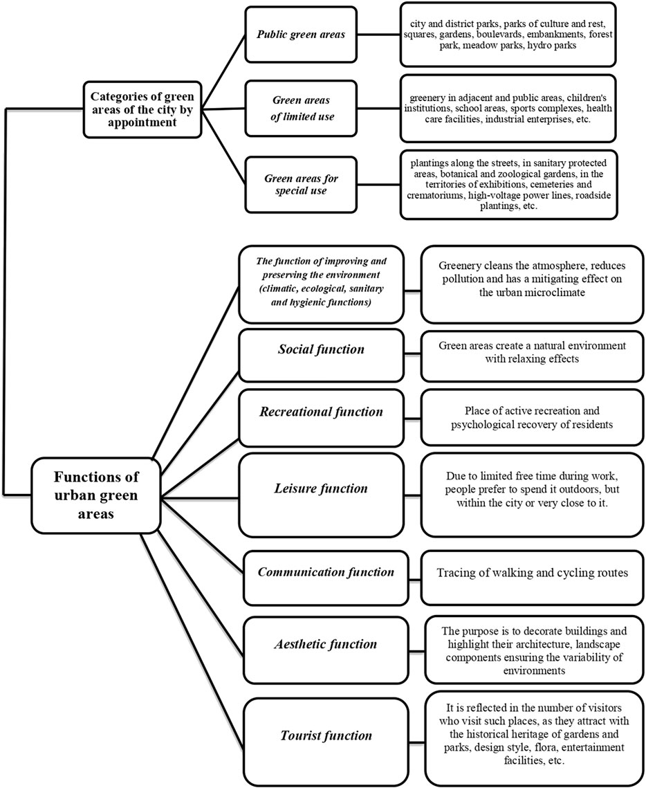
FIGURE 1. Categories and functions of city’s green areas (compiled according to data) (Degorska (2004); Cianga and Popescu, 2013).
2.2 Methodical Background
The authors used general and specific scientific methods in their study to establish the spatiotemporal dynamics of the UGAs functioning, their infrastructure transformation, and the expansion of their functions based on the example of Kharkiv. The authors applied the following methods:
• IInduction and deduction methods (for logical understanding and processing of available data and information about UGAs, their state, functions, and transformations).
• IComparison method (the authors used this method at almost all stages of the study to determine the current state of the UGAs and compare their development level).
• IMethods of analysis and synthesis (to study the individual components of the UGA and form a holistic view on the UGA features in Kharkiv),
• IRetrospective method (to analyze the plans of Kharkiv for different time periods and describe the objectives and goals of the Development Strategies of Kharkiv).
• IVisualization method (the authors used this method in combination with the graphical method to manifest the dynamic changes in the UGAs for different time periods).
• IContent analysis method (to analyze the spatial changes and transformations of the UGAs of Kharkiv and investments volume in the park areas development of the city in 2020).
GIS analysis is the most effective tool for establishing the current state and monitoring the spatial transformations of the UGAs.
2.2.1 Backgrounds and Conceptual Framework
Urban territories are one of the most dynamically changed, existing land use types. Global mapping and thematic classification of urbanized areas are challenging because of the lack of spatiotemporal information in the traditional (analog) sources concerning changes in these areas. Derivative tracing of the UGAs’ dynamics within the mentioned built-up territories makes this necessity even more complicated. In this regard, satellite image processing with further involvement of Geoinformation System (GIS) tools can hardly be overvalued. So far, there have been many examples of this technique’s implementation realized on the global, national, regional, and local scales. Existing digital layers, made using global satellite images, are reported in relevant papers (Bartholomé and Belward, 2005; Gamba and Herold, 2009; Potere et al., 2009; Gonga et al., 2013; Ban et al., 2015). A quite representative paper of research on the urban green footprint at the national scale is an introduction of an innovative algorithm. The approach of this algorithm is to separate the fraction of green areas extracted from Landsat 5 TM/8 OLI global coverage using data mining tools (Roy et al., 2014; Kuang and Dou, 2020). Derivative results of the remote sensing applications could be employed at the regional level of UGA studies, where the research area would cover several urban locations at once within a region not large enough. Thus, we have to refer to a relevant example (Tyrväinen et al., 2005). There was little research affiliated with the local level, the one-city scale, and considering the limits of this text space, we have to recall only some Successful city, 2021 examples: Kunming (southwestern China) (Zhou and Wang, 2011), Delhi (India) (Gupta et al., 2012), Deyang (China) (Ma et al., 2018), Shanghai (China) (Du et al., 2017), Fuzhou (China) (Cai et al., 2019), and Karachi (Pakistan) (Batool et al., 2019).
If urban green areas are a subject of some integrative practice for supporting managed development of a city, the well-being of its residents, and the sustainability of a whole urban ecosystem, they should be described by a number of qualitative and quantitative parameters. Using only GIS without updated satellite or airborne data could produce limited results and conclusions (Gemann-Chiari and Seeland, 2004; Ragab, 2014). Mentioned parameters can be obtained only as a united result, as we already emphasized above, if applying remotely sensed imageries and various options of GIS functionality, with which the descriptors that are efficiently useful in objective evaluation of spatial green and built-up patterns and their relationships can be obtained (Senanayake et al., 2013; Chen et al., 2014; Du et al., 2017; Lang, 2018; Batool et al., 2019).
Some combined approach introduced in the two consequent publications was consisted of processing the satellite data of high resolution together with employing regional airborne survey results (Schofer and Lang, 2006; Lang et al., 2007), and it can be considered as the application at the local level too because it toughly targeted only the territory of Salzburg, Austria. Using QuickBird imageries, these authors provided the object-based classification approach and then calculated some weighted indexes as a parameter describing the ratio between the built-up and green areas. This approach was then developed further in relevant studies that presented the definition of green indexes and outlined a neighborhood level for the index computing because a neighborhood is an areal outline for greening practice (Gupta et al., 2012), while monitoring of UGAs in Salzburg was continued after employing QuickBird by WorldView-2 (2010) and Pleiades-A (2015) resulting imageries (Lang, 2018). These examples that illustrate extracting green regularities from the satellite data processed by GIS present representative case studies for the content of our study. Herein, we also aim to represent those formalizing tools that can effectively identify sustainable spatiotemporal dynamics of UGAs depending on various urban configurations.
The traditional in situ measurements of urban green areas usually provided the common city scheme of 2D distribution of trees over a given territory. Clearly, it was not only time-consuming but also labor-expensive. Using the modern remote sensing approach, the same thematic research [2D structure, distribution and change detection (CD)] can be effectively accomplished with several spectral bands and numerous vegetation indexes of the Landsat TM data (Chen and Gillieson, 2009), if only we do not have to enter into the 3D domain of urban greenness, where other sensors, than those mentioned above, should be involved—Light Detection and Ranging (LiDAR) software and hardware (Huang et al., 2013). If involved in urban studies, this technique can detect, extract, and model various unique features due to the ability of a scanning laser to generate a 2D/3D view of existing environmental reality. This characteristic of the LiDAR approach luckily correlates with the ability of contemporary GIS platforms to simulate the urban environment as some 3D scenes.
Even if we have a background in LiDAR applications for urban studies, including relevant options for green volume analysis, we had to avoid the techniques of 3D modeling and analysis due to the lack of airborne LiDAR data covering our area of interest (AOI). Nonetheless, we employed the functionality of change detection in LiDAR point clouds for applications to the photogrammetric clouds extracted from the Landsat global coverage data. Our earlier developed CD-based functionality targeted for LiDAR surveys over urban areas can be explained. This tool processed and compared two point clouds (primary and secondary). It delineated the exact locations of changes and provided a report with change details. This tool was strongly based on the feature extraction functionality because the changes are presented as 3D models. Its technique consisted of the following steps: 1) processing and classification of the two sets of LiDAR data collected in two different time periods; 2) comparing points assigned by the classes of buildings and trees, finding geometric changes, and saving a report as a database file; 3) providing additional info about the found changes; 4) displaying both changes and point cloud data in Cesium 3DTiles. Later on, we adopted this technique exactly for photogrammetric point clouds if a given point density satisfies the processing requirements. Nonetheless, CD as a cloud-based method is presented in this research as a supplementary one, while the change detection of UGAs, grounded on the thematically classified images (taking only satellite image R, G, B bands for CD) as with their pre- and post-processing, has been chosen as a primary method. We only used the 2D visualization of urban green pattern changes to remain within the objective and scope of our research, which is to evaluate changes in the urban stand loss (USL) within an official boundary of a large city for a long period of time (2000–2020) as on a yearly basis. The outlined research task can be resolved on the basis of our original multifunctional urban remote sensing (URS) approach (Kostrikov et al., 2020a; Kostrikov et al., 2020b) combined with the strong spatial aspect of a full-format GIS-platform functionality.
2.2.2 Overall Approach and Data
Our research aims to study the long-term dynamics of UGAs in a large city. In particular, it focuses on providing the originally combined URS/GIS approach resulting in CD identifications within UGAs. An applied objective of the study was to identify the total green area covered with urban vegetation in a given year, then spatially compare it with a relevant characteristic related to the following year, and finally estimate either negative or positive changes per year. The CD identifications have been based on key points introduced in relevant fundamental works: image preprocessing, thematic classification, post-processing, and accuracy assessment (Anderson et al., 1976; Strahler et al., 2008).
The initial data as preliminarily processed satellite imageries, which overlap a period of more than 20 years (2000–2020), were obtained from the Earth Observing System (EOS) Data Analytics company (https://eos.com)—the global and the biggest Ukrainian provider of remote sensing data sources. While choosing the mentioned URS data, we considered the existing references due to the applicability of the Landsat images as the results of the medium-resolution sensors broadly acceptable and preferable for both monitoring the areas not large enough or for a selected city (Kaplan, 2019) and mapping forest vegetation and change detections in its various classes itself, through diverse approaches, within the different environmental zones (Lu et al., 2004; Makela and Pekkarinen, 2004; Banskota et al., 2014; Millard and Richardson, 2015; Schott et al., 2016).
The Kharkiv urban green areas were defined by green coverage parcels of open space in urban forests, parks, gardens, and residential areas and along roads and other traffic corridors. The extent of UGAs for Kharkiv and its nearest suburbs was extracted from 13 datasets of Landsat 7 (ETM+) multiband imageries (30 m resolution per pixel, the period of 2000–2012) and from eight datasets of Landsat 8 (OLI/TIRS) (15 m resolution per pixel, the period of 2013–2021). All datasets included L1T images. Table 1 shows a dataset extraction, a path/raw combination, a sensor type and a path on a circle day, and common combinations of bands plied to a sensor.

TABLE 1. Landsat datasets from which the extents of urban green areas in Kharkiv have been retrieved.
All data sources were obtained from the EOS satellite images of the low-/average-/high-resolution repository through a web link https://eos.com/landviewer/?lat=49.99719&lng=36.25102&z=10 and a relevant web interface (Supplementary Figure S1). The imageries were already set up as systematic-ortho satellite imageries and computed for pan sharpening. Generally, we employed the most suitable images, cloud free and taken from the same month or as close as possible. We selected almost all Landsat datasets during a warm season of a corresponding year, while a certain date was chosen due to the condition of cloudiness of fewer than 5%. The only dataset accepted as inaccurate was the Landsat 8 image of 16 March 2015. This image exposed no green alterations compared to the previous year (2014), while the CD processing technique was applied. Therefore, we had to complete a given pair of years as “2016 vs. 2014” and identify changes within this period.
The image processing results were compared for data accuracy assessment with various land-use, urban, and human geographical layers available from the Open Street Map (OSM) community through a web link https://download.geofabrik.de/europe/ukraine-latest-free.shp.zip.
Thus, through chosen data, conceptual frameworks, and the elaborated overall approach as URS/GIS, we provided the research focus on the green areas change detection in response to expansion of built-up areas and urban infrastructural networks. The CD techniques were accomplished primarily by land use/thematic classifying mapping (e.g., Yang et al., 2003) and, secondary, within a few selected year pairs by comparing relevant photogrammetric clouds preliminary extracted from the same data sources. The second CD-processing option was chosen for data accuracy assessment only. This change detection pipeline was a derivate of our original CD technique briefly described above due to LiDAR point cloud processing. The upgraded versions of the EOS geospatial web services, LandViewer (LV, an imagery browser with 700 million km2 of imageries, 14 built-in spectral indexes, and with an option of a few seconds only to find a required image) and Forest Monitoring (Supplementary Figures S2, S3), were employed for preprocessing, processing (supervised classification and thematic classification mapping), and post-processing. This software implies user’s customization for specified research and developing. We performed such customization, while the CD technique was applied for the satellite time series data. The Landsat time series CD algorithms (Jeevalakshmi et al., 2016; Zhu, 2017) embedded in the LV imagery browser were one of the key components of the overall processing approach (Figure 2). The flowchart blocks of key nodes have been selected in bold in this illustration. Necessarily, some common principles due to the urban greenness classification with indexes have been applied (Tigges et al., 2013). The LV Time Series Analysis (TSA), as some summarization of Landsat image processing results, finalized these processing procedures, and allowed us to analyze those alterations in UGAs which occurred in years and produce derivative classifications based on the primary supervised classification. The latter employed yearly Normalized Difference Vegetation Index (NDVI) threshold values and generated the changes raster. The output of the derivative TSA classification was the number of urban stand loss (USL) polygons for 2000–2020.
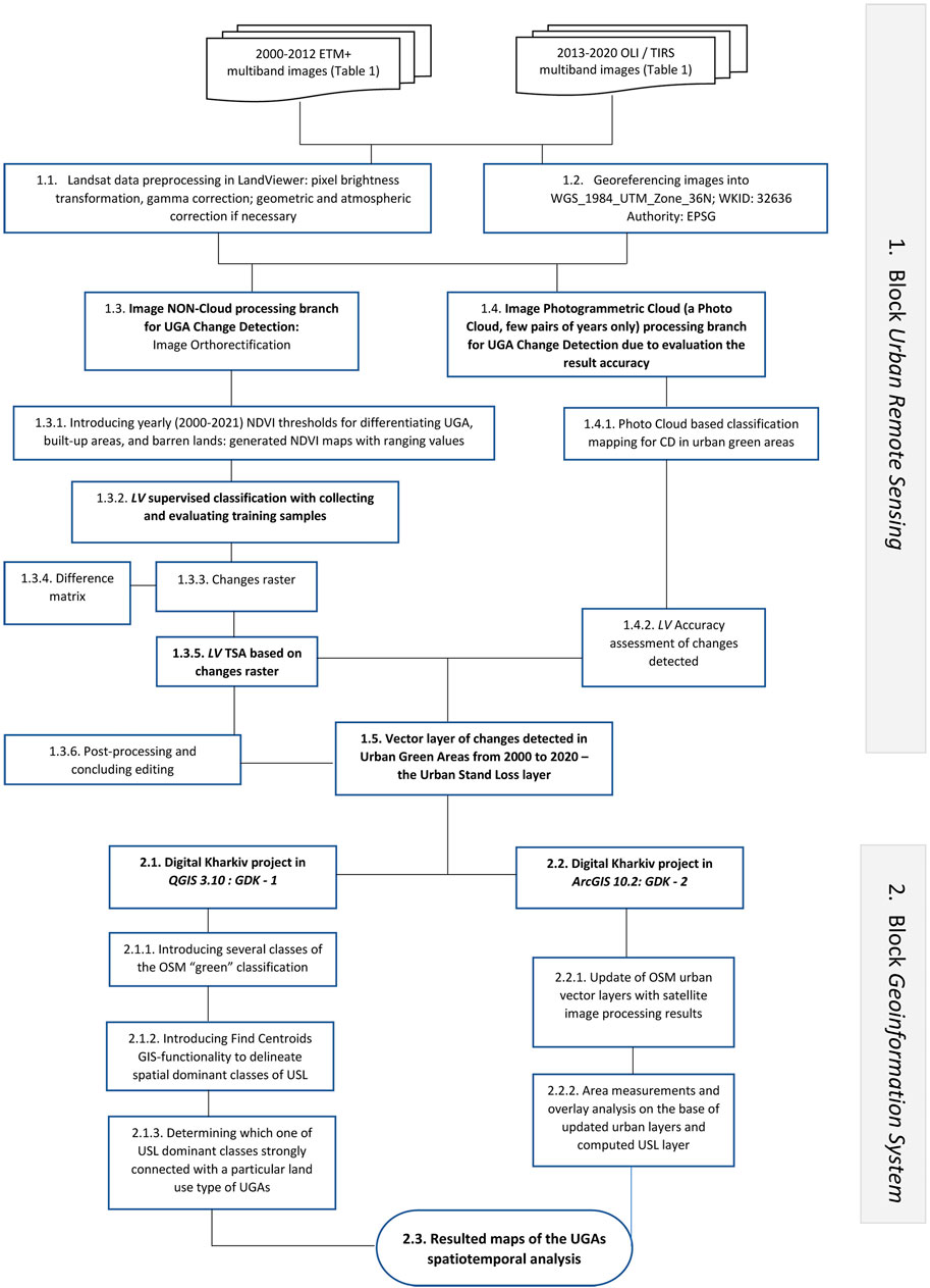
FIGURE 2. Overall flowchart of the combined URS/GIS approach to the spatiotemporal analysis of urban green areas.
General processing procedures can be divided into two hyper-blocks: URS and GIS. The first block was mentioned earlier. Within the second block, two alternative GIS projects of the “Green Digital Kharkiv” (GDK-1, GDK-2) were completed: one on the open-source QGIS 3.10 software platform on the basis of OSM layers mentioned already (GDK-1) and another one in the ArcGIS 10.2 interface (GDK-2). If the first one was completely combined from external layers, the second one implied its innovative update from satellite imagery processing completed by the LandViewer imagery browser team for several recent years (https://eos.com/landviewer/?lat=40.68921&lng=-74.04448&z=18&preset=highResolutionTmsSensors).
2.2.3 Methods and Techniques
The overall flowchart in Figure 2 provides an overview of the used methods and techniques. Block units 1.1–1.4 belong to the hyper-block of urban remote sensing, while the 1.5 block unit is a transitional one from URS to the Geoinformation System hyper-block. The latter consists of 2.1–2.3 block units. Some of the block units that belong to both hyper-blocks have been briefly examined already in the previous section of this paper, while the other ones are introduced in this section.
All procedural block units presented in the illustration belong to both the LV image browser and the Forest Monitoring web-service functionalities, which are embedded in a pipeline normally hidden from the user. Nonetheless, there is a broad range of this software customization according to a particular research task. For example, while providing small-scale monitoring (the most preferable for this image browser) within a large AOI selected in the western part of the United States, a user is free to choose a necessary band combination to obtain either a certain vegetation index or some other customized results (Supplementary Figure S4).
Just as in this example presented, we performed customization of the LandViewer software functionality according to block units 1.1–1.4, which are in the overall flowchart Routine Landsat image preprocessing accomplished in the LV interface in block unit 1.1. Because almost all Landsat datasets are provided in the georeferenced mode, the content of block unit 1.2 implies geocoding our own data with at least ten ground control points properly distributed over our AOI selected. After obtaining the necessary GPS-based coordinates, the datasets were reprojected according to the projection description given in block unit 1.2 (Figure 2). Image orthorectification (unit block 1.3) begins a whole branch of Image NON-Cloud processing for CD in UGAs, as it provides prerequisites and conditions for further processing, classification, and post-processing in 2D mode within 1.3.1–1.3.6 sub-unit blocks as well as 2D GIS mapping through block units 2.1 and 2.2 of the second hyper-block.
The mentioned flowchart branch was planned to be compared with the Image Photogrammetric Cloud branch, which is started by block unit 1.4, the only one within this flowchart where 3D processing has been implemented. Photo clouds have been extracted by the EOS Platform analytical tools from KOMPSAT-3A high-resolution imageries, HRI (0.4 m per pixel) available from the EOS HRI repository from https://eos.com/landviewer/?utm_source=Email&lat=41.33283&lng=-93.19336&z=4&id=S2B_tile_20211102_13TEF_0&b=Red,Green,Blue&anti=&preset=highResolutionSensors. Pairs of years have been chosen exclusively due to these datasets availability: 1) 2014 (a primary target for CD) and 2016 (a secondary target) benchmark; 2) 2017–2018; and 3) 2019–2020 only. The EOS analytical tools processing these HRI datasets have been based on these dataset specifications (Lee et al., 2010; SI Imaging Services, 2016). While adjusting our original LiDAR point cloud processing technique for feature extraction and digital elevation model generation (DEM-G) from photo clouds, we took into account existing solutions exactly in the subject area of forestry, which would include some parallel applications of airborne laser scanning and satellite photogrammetry (Pearse et al., 2018). A small parcel (around 2.5 ha) located in the northern part of our AOI, which was selected for UGAs CD checking based on photo clouds in the 2014–2016 benchmark, has been visualized in the customized EOS platform web interface. This visually illustrates the photo cloud-based classification mapping change detection in UGAs on a yearly basis on a large scale (Supplementary Figure S5). Defined alterations have been marked as the polygons bordered by red lines and with red nodes in their vertexes.
From sub-block unit 1.3.1, the key flowchart branch of CD for UGAs starts, and it is implemented in the 2D mode only. Because two satellite sensors were involved in our case (Table 1), the “collaborative scheme” is presented (Pax-Lenney et al., 2001), according to which the content of classification should be trained beyond the extent of the initial training dataset (sub-block unit 1.3.2). Sub-block unit 1.3.1 implicated computing a normalized difference vegetation index (NDVI) as both satellite sensors employed in our research collected key multispectral bands [(R, G, B, and Near Infrared (NIR)]. NDVI values were calculated by the commonly accepted routine formula:
Values calculated through Eq. 1 were accepted as basic parameters for providing supervised classification within block unit 1.3.2 by the LV image browser analytical tools and differentiating only three basic classes of 1) urban forests (urban green areas), 2) built-up areas (infrastructural networks), and 3) barren lands. While customizing the LV software for computing NDVI by choosing its thresholds according to the research objectives of our study, we considered existing references to both the forest vegetation and the basic urban land use (ULU) classes reliably mirrored by NDVI (Immitzer et al., 2012; Tigges et al., 2013; Li et al., 2016). The key assumption is that the NDVI value can provide us with a cue, on the base of which the urban parcels land use was reclassified from the first class to the second or third ones. Moreover, this cue allowed to differentiate urban forests from both parks and gardens, as well from UGAs subclasses.
According to the datasets we had to work with in the NDVI analysis (LANDSAT data of medium resolution: 1 pixel = 2,645833E-7 km), an area, which is even only relatively large enough (as on the example given above—Supplementary Figure S4) cannot be outlined due to sharp loss of accuracy. Therefore, an image browser recommends restricting an urban area as an NDVI-AOI to 150 km2 only, which is 2,333 times fewer than a whole AOI (Figure 3). Thus, we had to select three NDVI AOIs (150 + 100 + 100 km2) in order to cover all Kharkiv urban territory in its official borders; for example, one more part of the AOI was selected for the northern part of the urban area, where the largest urban forests were located (Supplementary Figure S6). Another problem of this vegetation index estimation consisted in that fact, according to which default LV NDVI TSA-calculating tools produced this index calculated output bound to the LANDSAT-8 sensor for the temporal range of July 2015–July 2020 only, although we used data for the custom period of May 2000–September 2020 (LANDSAT 7, 8 sensors) according to Table 1. Such NDVI progress schedule for the central urban territory of Kharkiv, we have just referred to above, is illustrated in Figure 4. Thus, we had to apply to the LV Upgrade option, which allowed us to provide the user’s customized software upgrade, what we accomplished for the backend (with C#/Python coding) and the frontend (with JS coding). This enabled performing processing that concluded the whole long-time research interval to calculate NDVI in May 2000–November 2014. The negative NDVI values were accepted as built-up areas and barren lands, while the positive ones as UGAs. As we already mentioned, various VGA sub-classes were distinguished within these positive values.
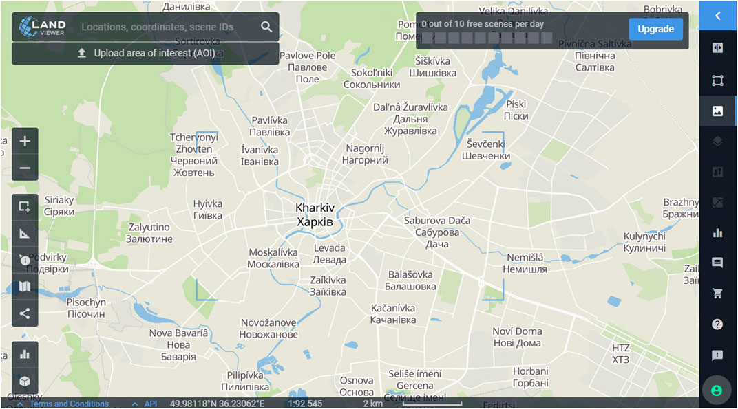
FIGURE 3. The central part (not more than 150 km2) selected in urban territory for calculating aggregated NDVI values in a long time interval (2000–2020). The LandViewer image browser interface.
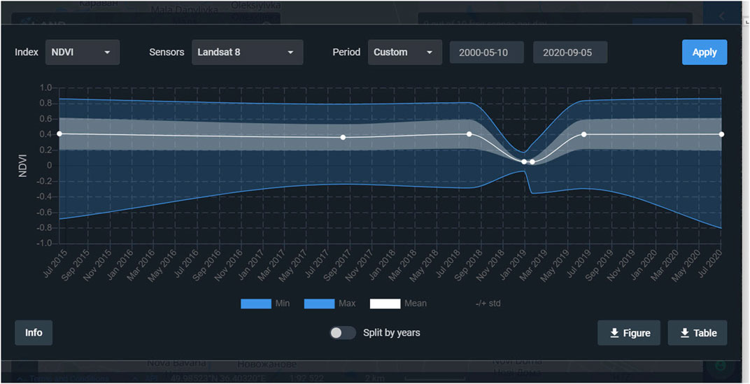
FIGURE 4. The aggregated NDVI progress schedule in July 2015–July 2020 for the central part (Figure 3) of the Kharkiv urban area. The graph is presented in the LandViewer image browser interface.
Sub-block unit 1.3.2 provides initiation of change detection based on comparing results of multitemporal classifications and on preprocessing steps made in block unit 1.1 (procedures that allow correct comparison of the pixel spectral brightness). For the supervised classification, all training parcels for pixels were defined outside and inside these parcels. The nearest neighbors algorithm (NNA), k-nearest neighbors (kNN), was applied within the frameworks of “hard classification with supervised training” (Franco-Lopez et al., 2001). The algorithm consists of the following approach. If training parcels and their neighboring parcels are located in the united spatial extent and belong to the same class, then the parcels are defined as this class in any spatial extent. If the area unfits to the given class, it is defined as an unclassified one in finalizing the 1.3.2 sub-block unit classification layer. The classified maps are the direct result, which is a subject to some generalization methods—either smoothing, aggregation, or both can be provided. The result as thematic changes is provided by the 1.3.3 Changes raster sub-block unit, which is a derivative image of a LANDSAT dataset, and the 1.3.4 difference matrix, which describes the preliminary defined changes in a table form.
The 1.3.5 sub-block unit LV TSA based on changes provides a repeated TSA NDVI calculation. However, it is based on a preprocessed image as in previous sub-block units and uses a derivative raster. The NDVI yearly maximum mapping results were classified and converted in the feature classes. It is an alternative mode to sub-block unit 1.4.2 (based on photo clouds). For the reasons of accuracy, we randomly selected sample parcels or calculated UGAs CD polygons, in order not to not impact training areas of the classification. In both cases, LV Image Accuracy Assessment functionality was employed. In addition, the total accuracy of change detection through block unit 1.3 of the flowchart was estimated as 87–90%, while the accepted minimum accuracy for urban remote sensing is around 85% (Anderson et al., 1976).
Sub-block unit 1.3.6, post-processing and concluding editing, closely relates to accuracy estimation and mainly provides sieving (remove or unite small CD polygons and classification errors as a group of few pixels), clumping (aggregation and smoothing boundaries of small parcels), and majority/minority analysis (assigning a defined user’s “central pixel” either to the class of most pixels or to the minority of pixels in the neighborhood).
The calculations based on photo clouds within the block unit 1.4 of the flowchart values of USL appeared to be quite comparable to those estimated within the main workflow branch (Table 2): 1) 2014 (a primary target for CD) and 2016 (a secondary target) benchmark = 63067 m2 (vs. 60462 m2 in the block unit 1.3, thus with 4.3% of a difference); 2) 2017–2018 benchmark = 67114 m2 (vs. 63735 m2 in block unit 1.3, with the same 4.3% of a difference); and 3) 2019–2020 benchmark = 112950 m2 (vs. 106583 m2 in block unit 1.3, with almost 6% of a difference). Generally, it is quite reasonable to emphasize that the 3D-processing branch (block unit 1.4) does not produce overestimated CD values due to USL, but the 2D-processing branch (block unit 1.3) generates underestimated values, also found in relevant studies (Huang et al., 2013; Ma et al., 2017). Nonetheless, due to the lack of HRI images, the study was limited by 2D processing.
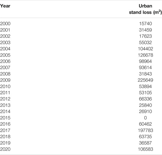
TABLE 2. Yearly USL values in 2000–2020 within the official urban territory of Kharkiv (a graph view in Figure 7).
The resulting block unit of the URS hyper-block (Figure 2) is the block unit 1.5—vector layer of changes detected in UGA from 2000 to 2020, the Urban Stand Loss Layer. This block unit is a transitional one to the GIS hyper-block, as already mentioned above. It resulted in a layer of polygon features as the detected changes in Kharkiv UGAs (Figure 5). It can be seen clearly from this illustration that a major number of urban stand loss polygons (USL was accepted as a united criterion of tree loss in the region according to the approach implemented) have been identified outside the official border of the Kharkiv urban area. They are located in the main forest regions of the northern and northwestern territories of city suburbs and rural areas. The total USL value, which corresponds to the united USL within the city border and beyond it in the nearest suburbs, which finalizes the URS hyper-block illustration of USL parcels, is 622 ha (Supplementary Figure S7). That part of the loss parcels, which was located in the nearest city suburbs beyond the city border, has been examined and compared with available regional data of deforestation in the EOS Forest Monitoring web service (Supplementary Figure S2). However, this service does not allow directly estimating the urban vegetation because of the relevant lack of data. Further in our study, we eliminated all stand loss areas outside the city border and only included areas within the city.
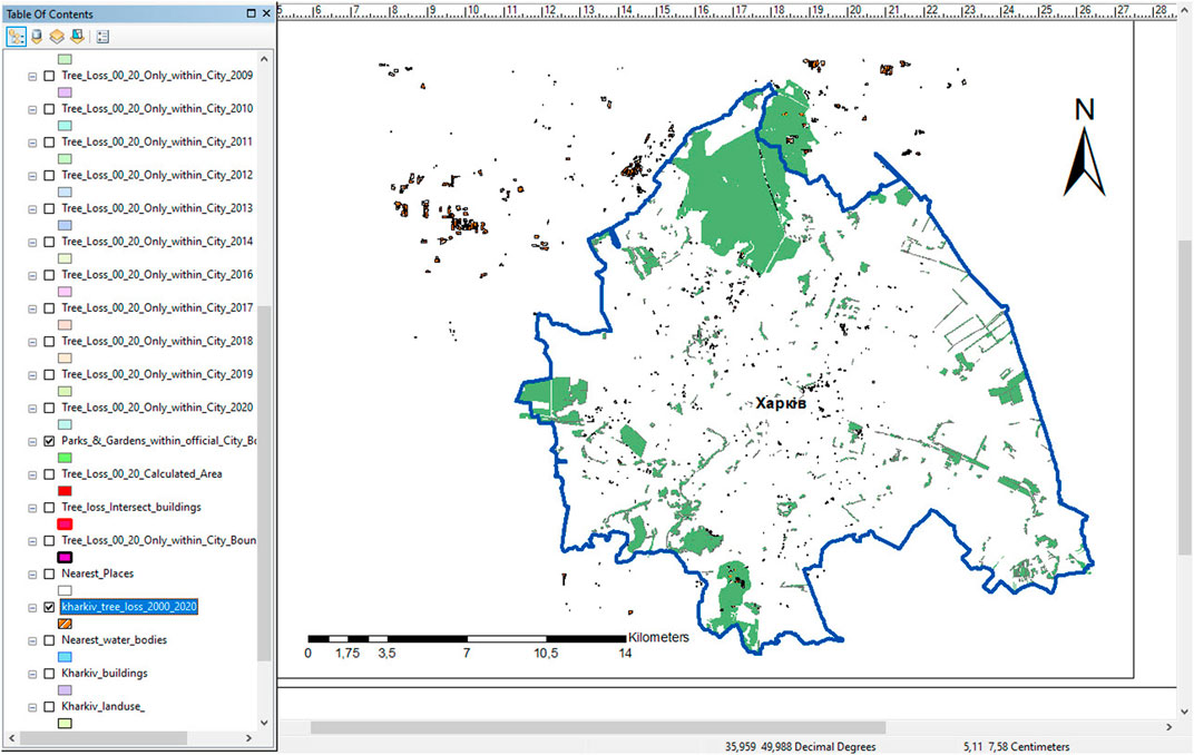
FIGURE 5. Changes detected as the stand loss in urban green areas of Kharkiv and the nearest suburbs as an overall loss in 2000–2020. The Green Digital Kharkiv project in the ArcGIS 10.2 interface (GDK-2).
Two already alternative Green Digital Kharkiv GIS projects mentioned above were completed on two different platforms: block unit 2.1 starts the QGIS branch (GDK-1) of the Geoinformation System hyper-block with sub-block units 2.1.1–2.1.3, while block unit 2.2 starts the ArcGIS branch (GDK-2) with sub-block units 2.2.1 and 2.2.2. We do not introduce in peculiar detail the thematic content of these units because they represent the standardized GIS -analysis and spatial pattern delineation with well-known tools for most GIS users (Craser et al., 2017). Nonetheless, some procedural aspects are highlighted at the end of this section. Several resulting derivative maps visualized in two GIS platforms summarize finalized results of processing, modeling, and analysis for a whole workflow. It is the content of block unit 2.3, which means the UGAs spatiotemporal analysis output (Figure 2).
To the mentioned extent, the content of the resulting maps should be combined on the basis of areal measurements, overlay operations, and delineation of territories of the USL values per year. According to the overall workflow (Figure 2), the USL polygonal feature layer was initially obtained as an aggregated one, where a year of loss could be distinguished in the standardized Digital Number (DN) column of the layer attribute table, in which one- and two-digit integers corresponded to a certain year in the 2000–2020 range. After updating the latest URS sources, the Digital Kharkiv project was created on the ArcGIS 10.2 platform. The Selection => Select by Attributes tool was applied, and the USL layer was partitioned for 20 layers on the basis of 20 selection sets of the Year attribute. The year 2015 was excluded from the series according to the explanations provided above.
There were no tools to measure the metric values of polygon feature areas in the first hyper-block of our workflow (Figure 2). The initial areal measurements could be provided after importing the resulting layer (block unit 1.5) in the ArcGIS 10.2 interface and completing the following pipeline: ArcToolbox=>Spatial Statistics Tools=>Utilities=>Calculate Areas.
Delineation of the USL spatial patterns within the city boundaries finalized our methodical workflow. Relevant techniques employ the enhanced OSM data due to the urban land use, which are available by the QGIS module, QuickOSM (a data query is provided within the spatial extent of Kharkiv) if we operate within the GDK-1 GIS project.
In order to add to attribute tables of each green sub-class of the USL data, that is, a number of stand loss polygons in each green sub-class, it was necessary to convert polygonal features into a centroid, a point feature of an initial polygon. For these objectives, we applied the QGIS tool, Convert Geometry type. This tool allowed converting all polygonal features in the corresponding centroids with necessary georeferencing. A new layer of the urban stand loss as the layer of centroids has been generated, which allowed distributing all centroids to seven dominant USL classes of the point features within the 3-year period marked as “January 1 of the first year–January 1 of the fourth year.”
Afterward, we applied the tool count points in polygons to summarize a number of centroids in the various LU classes, as in the green and non-green ones. This classification has been based on the OSM data. The software prescribed the mentioned sums of centroids to the attribute table of the green land use in the Numpoints field. The same procedure was completed for the layer of the city’s existing wards.
Then, it was necessary to deliver some attribute information from the centroid layer to the vector polygonal layer of the green land use. We used the USL data per year, which would allow building a map of the stand loss dominant classes bound not to the point features (USL centroids) but to the polygonal spatial features, LU polygons, in order to obtain further in this way spatial correspondence between the urban stand loss and a particular class of green LU. Exactly, this procedure provides prerequisites for the USL spatial pattern delineation.
For these purposes, firstly, we inserted in the centroid layer attribute table ID of those LU polygons, in which centroids are located, and completed it with the tool Join attributes by location. Within this link of a whole pipeline described here, we obtained a map of 10 green sub-classes corresponding to the USL dominant classes.
In the next step, we calculated the modes, dominant USL values for all green LU polygons according to their ID. We did it with the Field calculator tool and the majority function. The query expression was completed as follows: majority (year, group_by: = united_id). In this way, those polygons, which were hit by centroids, obtained USL values per certain 3 years (the USL dominant temporal class mentioned above). Then, finally, the obtained dominant values of the centroid layer were delivered into the polygonal green land use layer by the tool of Join attributes by field value. Thus, it enabled recognizing which dominant classes were strongly connected with some particular green LU types. This map is illustrated in the Results section of this article.
In the final step, the results of all previous steps were overlaid with the centroid layer, colorized by the unique value method (UVM). In this way, the spatial dominant classes of the urban stand loss in Kharkiv were obtained. It is a key output of the CD-based spatiotemporal analysis provided in our study.
3 Results and Discussion
3.1 General Features of Kharkiv as a Study Area
Kharkiv is located in the North East of Ukraine, and it is the second-largest urban territory in the country. Latitude and longitude coordinates are 49° 59′ N and 36° 13′ E. The city’s total area is 350 km2, and it is gradually increasing because any natural barriers do not limit the urban expansion of Kharkiv. The city’s position among other cities and regions of Ukraine can be illustrated by the composite visual image of Copernicus Sentinel-2, source: geoportal “Ukrainian Forests.” (https://forestry.org.ua) (Figure 6). The city, with a population of just over one and a half million, is located contiguity to the steppe and forest-steppe ecoregions. Natural forests, which remain mainly in some areas on the northern and northwestern outskirts of the city, are dominated by oak and pine species, and spruce is the third predominant species. Supplementary species are lime, maple, ash, and acacia, while other species are dominant ones if soils are wet enough—birch, alder, willow, aspen, and poplar. These trees complete the species composition in urban forests, parks, gardens, and other green parcels mainly added by fruit trees. This composition can change significantly from one urban parcel to another one.
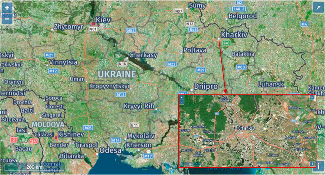
FIGURE 6. Location of the study area according to other regions of Ukraine (a source: the Ukrainian Forests geoportal https://forestry.org.ua/).
There is no unauthorized housing development in Kharkiv, a usual key factor of urban deforestation. Therefore, there are no high-density developed low-rise (2–4 stories) houses, and a dominant majority of dwelling houses are high-rise departmental buildings (9, 12, 16, 24 stories). Planned and authorized development regulates low-rise residential/commercial buildings, high-rise residential apartments, and traffic corridors. The city grounds are a complicated mix of urbanized soils and impervious surfaces. The distribution of UGAs is determined by urban forests at the city edges, green belts of parks and hardens in commercial zones, trees in residential urban parcels, and street trees.
The significant scale of capital and housing construction and the increase in the population of Kharkiv due to its development dynamics as an industrial and cultural center in Soviet times led to a significant expansion of the city’s boundaries. In 2012, the last changes in the city area took place, increasing by 14% (Resolution of the Verkhovna Rada of Ukraine, 2013). Today, Kharkiv is in the transitional stage to post-industrial development, which is also reflected in the planning structure, spatial zoning, urban space transformation (Niemets L. et al., 2018; Niemets et al., 2019a; Niemets et al., 2019b; Suptelo and Sehida, 2020).
Kharkiv is one of the greenest cities in Ukraine. It differs from other industrial Ukrainian cities. According to official data, which can be discussable proceeding from the results of our study, the total area of greenery in the city is 15.4 thousand hectares (Development Strategy of Kharkiv until 2020, 2021). Cities, where vegetation occupies less than 10% of the city’s area, are considered unsatisfactory in terms of landscaping, in case 40–60% of the situation is satisfactory (Komarova, 2006). Greenery in Kharkiv is about 44%. Each inhabitant of the city has about 106.7 sq.m of greenery at a norm of 50 sq.m, as determined by the WHO (Badiu et al., 2016). Throughout almost the city’s entire history, the local authority carried out active work on its landscaping, creation of squares and parks, gardens and boulevards, conditions formation for health improvement and recreation, and improvement of living conditions Kharkiv residents. The UGAs of the contemporary Kharkiv include 29 parks, 4 gardens, 150 squares and boulevards, and more than 500 green recreation areas. Fifteen objects of the nature reserve fund of state and local significance occupy an area of 467.7 ha (development strategy of Kharkiv until 2030).
3.2 Analysis of Changes in Green Areas in the Spatial and Functional Organization of the Territory of Kharkiv
During the history of Kharkiv, starting from the first documented plan of Kharkiv (1787) and the town-planning plan (1867), local authorities changed these documents according to the development and expansion of the city. The contemporary territorial organization of functional zones of Kharkiv is regulated by the main documents, particularly the Master Plan of the city, functional zoning of the city, the cadastral map, and so on. These documents, following the current legislation, are publicly available. The City Development Strategy (concluded for 10 years) and the City Program for Investment activities and Image Projects (concluded for 5 years, this is an example of the medium-term planning) reflect the state, problems, and prospects of the city development (Official site of Kharkiv City Council, 2021a). Over the last 30 years, four Master Plans of the territory of Kharkiv were proposed in 1990, 2004, 2013, and 2019. The city and the territorial organization of UGAs have changed significantly for more than 230 years. We analyze the spatiotemporal changes of the UGAs according to Supplementary Figures S1.1–1.12.
The first plan-map of Kharkiv is dated 1787. According to this cartographic material, the green areas were mainly suburban (Supplementary Figure S1A). The first urban plan of Kharkiv was developed in 1887. Accordingly, the area of Kharkiv expanded in all directions and included most UGAs. They were dispersed throughout the city and located in both the center and peripheral areas. It indicates the city planners’ attention to residential and industrial areas and the areas with infrastructural and social functions (Supplementary Material S1A, Supplementary Figure S1B).
All the subsequent urban plans were associated with a strong pace of industrialization. In particular, the Master Plan of the city of 1925 highlights the 500 m green area between industrial and residential buildings (Bagaliy and Miller, 1993) (Supplementary Material S1A, Supplementary Figure S2). This city plan paid attention to the development of park and recreational areas near large enterprises to offset the negative impact of pollutant emissions and implement the population’s recreational and health function in the newly developed residential areas. There was a visible expansion of green areas and their reorientation to peripheral areas. The next Master Plan of Kharkiv in 1940 (Supplementary Material S1A, Supplementary Figure S3) demonstrates the fragmentary park and recreational areas in the city center and quite large recreational areas in the peripheral areas. The next Master plan of Kharkiv, placed on the terms of free access, was created in 1990 (Supplementary Material S1A, Supplementary Figure S4).
For almost 50 years, the city’s area has been transforming. Residential areas and transport infrastructure have been developed. The city’s recreational areas were expanded, and significant central park and recreational areas have been formed, serving all city districts. Starting from the 1990s, when creating the Master Plan of the city, the designers began to consider not only its territory but also the situation in the regional settlement system (with suburban and green areas).
One of the interaction results of the central city with its surroundings is the territorial growth of buildings towards each other in terms of urbanization processes. The “green belt,” which must be stable and play a key role in the environmental framework, is expanding from both the “center city” and its satellites. Each city has its own official territory within the delimited, demarcated, and documented boundaries. Such territorial growth of buildings is usually not provided in the Master Plans and schemes of district planning.
The Master Plan of Kharkiv, 2021 manifests the following structure of recreational areas: culture and rest parks occupied 442.0 ha; city, district parks, and gardens of residential districts had 228.0 ha; squares occupied 448.0 ha; embankments and boulevards had 258.5 ha; and water parks and meadow parks had 434.0 ha. This plan provided the expansion of the recreational area in the areas of new urban construction (Supplementary Material S1A, Supplementary Figure S5).
Nowadays, the most relevant Master Plans are the plans for 2013 (Supplementary Material S1A, Supplementary Figure S6A) and that with the changes made in 2019 (Supplementary Material S1A, Supplementary Figure S6B). During these 5 years, Kharkiv’s recreational areas have changed significantly. The rapid area reduction was concerned to the territory of the “Lisopark” in the north of the city, Oleksiyivsky meadow park, Hydropark, the greenery area in the park zones of the city. These processes are mainly related to the infrastructure development in park areas and housing construction. Parts of park areas, particularly unused cemeteries, are sometimes allocated for new construction. Parks and gardens of hospitals, formerly considered restricted areas, have a public status now.
Street greening is growing rapidly and characterizes the well-developed pedestrian and bicycle infrastructure. It has a greenery complex along the entire length, which will allow the streets to approach the status of urban “green corridors.” Furthermore, the transformed green areas of landfills and wastelands, forest protection strips, and railway diversion lines, which are not currently used, have potential elements of the green network.
The online GIS platform “Geoportal of the urban cadastre of the Kharkiv region, 2021” (Supplementary Material S1A, Supplementary Figure S7) allows viewing actual data on the territory planning of Kharkiv and the land resources cadastre of the city and the surrounding area. Such access to data is extremely positive for the city and allows obtaining information about the study area. The portal is still under development. Therefore, not all potential optional list of tools is available. However, there is no doubt that the UGAs are significantly compacted due to the residential area development and infrastructural transformations.
3.3 Analysis of the Spatiotemporal Changes of Urban Green Areas in Kharkiv
3.3.1 Common Issues and General Trends
We have already mentioned in the Introduction that, due to the information from the open sources (Hansen et al., 2013; University of Maryland, 2020; Global Forest Watch, 2021), Ukraine lost in the period of 2001–2019 up to 9% of the total national stand, if compared with the beginning of the millennium. This ratio mainly concerns rural forest stands. However, this common trend involves urban greening. Because no research based on a digital approach has not been performed for any city in Ukraine yet, our study can hardly be overvalued.
Thus, image differencing and classification/post-classification comparison introduced in the previous section resulted in several classified vector feature polygons. The latter indicated a change of the LU status based on the NDVI identification for a given urban parcel between two neighboring years as a shift of the first class of “forest” to the second or the third class of “non-forest.” This LU change has been accepted as a routine indicator of the deforestation phenomenon in a city. Any UGAs gain was not traced in the period mentioned. Hence, only a negative CD was identified. This can be easily explained by an extremely high cost and drastic lack of free urban lands in Kharkiv, as well as the actual absence of the sustainable municipal greening policy.
Additional accuracy assessment has been done by overlaying the vector polygonal features of USL (Figure 5) on relevant alternative data. The data were obtained from the Global Land Analysis and Discovery (GLAD) laboratory at the University of Maryland, which provides updated stand loss data on a yearly basis. In most cases, there is no information or only a minor one to the loss within urban territories. Nonetheless, this overlay on the GLAD layer of the tree loss in recent years in our region allows stating about a quite reliable register of CD identified in our study’s USL polygonal features to those ones, which have exposed deforestation in recent years according to this GLAD layer (Figure 7). Some defined mismatches can be explained by the fact that the GLAD layer was lately updated in 2017 only, while the original polygonal features of this study also reflected changes in the period of 2017–2020.
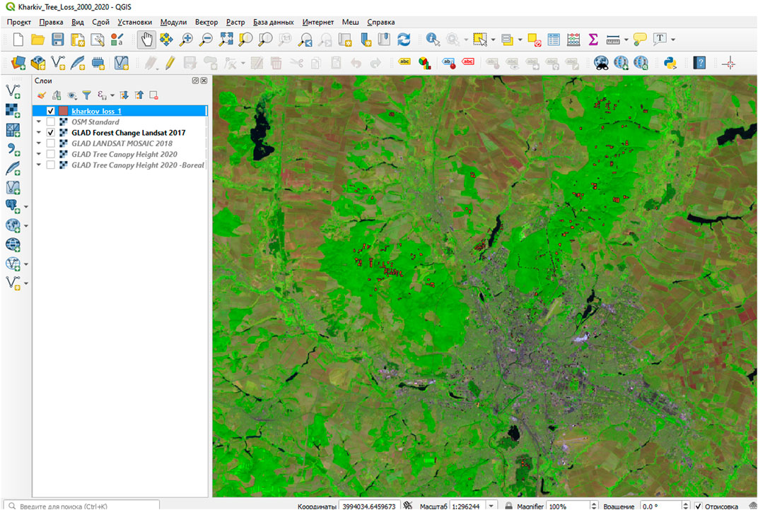
FIGURE 7. Overlay of CD identified in this study’s USL polygonal features on the GLAD layer of deforestation in the region.
3.3.2 Results of Areal Measurements, Overlay, and Areas of Urban Stand Loss Distributions per Year
We have emphasized in the methodical section that the USL layer was primarily calculated as an aggregated one. A particular year of loss could be selected by the standardized Digital Number (DN) column of this layer attribute table, in which integers marked a certain year in the 2000–2020 period (Supplementary Figure S8). The USL layer has been partitioned for 20 selections by the Year attribute (Supplementary Figure S9), with only 1 year excluded (2015).
The obtained yearly USL values were summarized as a total areal value through all USL vector features related to a given year (Table 2). The same data is presented in Figure 8. Thus, for 2015, the stand loss was traced only for city suburbs. Therefore, this year was excluded from the long-time analysis and exposed only zero values in this graph view. The probable cause was already mentioned above: the November 2014 Landsat dataset was compared with that of March 2015 (Table 1). Thus, the yearly NDVI maximus of these neighboring years might not be representative at all. If we eliminate from this graph this 2015 extremum, as not objectively grounded one, then three other low USL values are left: 1) those ones related to a set of 3 years, 2000–2002; 2) a value of 2008; and 3) a value of 2019. The first local negative extremum (2000–2002) could hardly be put in the correspondence with NDVI, calculated based on the Landsat 7 ETM+ by customized software that could build an NDVI map for 30 km2 only. Thus, we were unable to obtain a complete graph of the NDVI progress schedule for an area at least relatively large enough, as in Figure 4. A similar comment can be provided for the negative extremum of 2008. If yearly USL values may correspond with a long-term NDVI progress schedule, a more effective estimation can be done for the period of 2015–2020, where the NDVI is easily calculated by the basic LV image browser functionality. With this comparison, it can be clearly identified that the third extremum (2019) reliably correlates with the two NDVI progress schedules selected for two AOIs: one was in the central part of the urban territory (150 km2) (Figure 3), while the other is in its northern part (Supplementary Figure S6), where comparatively significant areas of urban forest extend with them natural large forest stands from the northwestern and the northern suburbs. The third minimal USL value of the graph (Figure 8) does definitely correlate with the NDVI schedule extremum in 2019 cold season, which can be clearly traced on both graphs (Figure 4, Supplementary Figure S10) and can be explained by existing and then local environmental conditions. Although two areas should be compared by NDVI by preferably 2D mapping (Gupta et al., 2012; Battol et al., 2019), not by graph views, aggregated NDVI values for the central AOI of Kharkiv (Figure 4) can be defined as somewhat lower ones (representative for dense built-up parcels) in comparison with the northern AOI, where definitely more UGAs are located (Supplementary Figure S10).
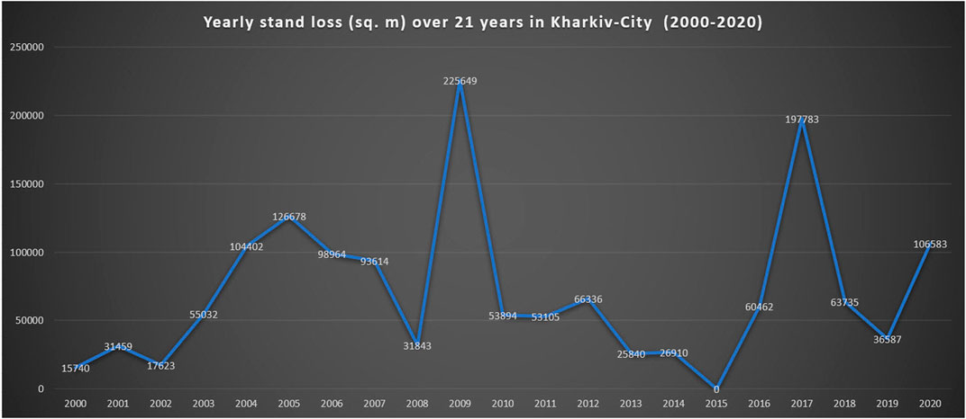
FIGURE 8. Yearly USL values in 2000–2020 within the official urban territory of Kharkiv (a table view in Table 2) (GDK-2).
Two Digital Kharkiv projects (GDK-1, QGIS; GDK-2, ArcGIS) on the alternative GIS platforms were necessary for the derivative processed result comparison, the interdependent validation, and the provision of the supplementary data accuracy assessment. Their completion allowed providing various GIS outputs, already mentioned above, where necessary areal measurements play a key performance. Thus, we already referred to a total stand loss of 622 ha in 2000–2020, which was defined for forest areas in the northern and northwestern suburbs together with inner city areas of parks and gardens. A total green area of Kharkiv, that is with tree stand existing now, (Kharkiv substantive provisions general plan 2004, 2021) was measured in GDK-2 project as 22400 ha, while a part of this territory located within an official city boundary is equal to 5040 ha with urban forests, with 1649 ha of urban parks and gardens only (Supplementary Figure S11). The mentioned values include only compact tree stand, but not, for example, single street trees, which belong to the Wood OSM sub-class. This, as the results of URS processing data of GDK-2 project, is quite comparable with GDK-1 based on the OSM sources. The value of 8589 ha was reported in the QGIS 3.10 interface for all LU subclasses of UGAs, which can be seen in the table of project content in the QGIS 3.10 interface (Supplementary Figure S12). It aggregates a total green area, not only those parcels, which are with tree stands. If we are interested in area distribution through all green subclasses, we can apply to the GDK-1 project with the OSM LU classification and define that forest, garden, and park subclasses make up 3601 + 76 + 959 = 4636 ha (Figure 9), while probably some ones from stand parcels appear in the wood subclass, which does explain the value difference of 5040 ha of forests, parks, and gardens in GDK-2 projects and 4636 ha in GDK-1.
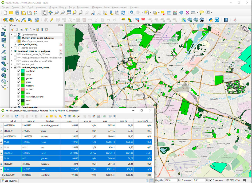
FIGURE 9. Area distribution of the OSM subclasses with tree stand in UGAs of Kharkiv: the total stand area of 4636 ha (GDK-1).
The values of GDK-1 and GDK-2 obtained using both innovative URS methods and reliable OSM sources clearly disprove the relevant official information of city authorities, according to which UGAs with stand in Kharkiv are as many as around 15400 ha.
From 622 ha of total loss detected in the AOI (Figure 5), the area within the city boundary exposed a loss of 149 ha only (Figure 10). A total USL of 101 ha was detected for urban parks and gardens, while for urban forests, it is 48 ha only (Supplementary Figure S13), which definitely may mean some more active built-up areas expansion to parks and gardens than to urban forests.
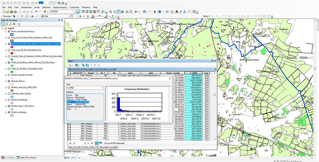
FIGURE 10. Calculated areas of 149 ha due to the total USL values in urban forests, parks, and gardens within the city’s official border only (GDK-2).
Nonetheless, the notable anthropogenic impact can be traced just in urban forests, particularly in the southern-western part of the AOI of our study. The following visual illustrates some modern construction of a building material factory on an urban lake bank with a huge sandpit built recently in the former urban forest (Supplementary Figure S14). Several USL vector polygons as the results of block unit 1.5 (Figure 2) are marked in that visual by yellow digits, identifiers of these polygons.
Areal measurements of UGAs in Kharkiv, computed on the basis of combined URS/GIS approach, prove that our city now sustainably exceeds the UN standard of the green space value per resident (30 sq.m): 50400183 sq.m (urban forests, parks, gardens–subclasses with tree stand calculated in GDK-2)/1447652 (a number of residents according to an OSM layer) ∼ 35 sq.m.
We also used the Intersect tool of the ArcGIS overlay analysis functionality while attempting to identify the USL causing factors. We chose a whole layer as input features and feature portions from its overlapping identical features, which allowed providing the attributes for an output feature class. Furthermore, we had to consider the references that considered the vector polygonal shapes as the ones affecting the overlay analysis efficiency (Zhang et al., 2021). With the overlay analysis procedures (a geometric intersection of the aggregated USL layer with the buildings layer as with the input feature class, Supplementary Figure S15), we disproved one widely existing regional opinion about a key cause of an urban stand loss such as an intensive and widespread built-up development in Kharkiv. There is 16 ha of the USL only during all these years directly because of housing development. Nonetheless, the result of the intersection of the USL layer with the streets and roads layers (understandably, with inputting some areal buffer around linear intersecting features (Zhang et al., 2021)) reported overlapped area up to 86 ha (Supplementary Figure S16), what may reveal one of the key USL factors in the period studied—the infrastructural development.
As already emphasized above, a common USL layer was partitioned for 20 selections (2015 was excluded) by a year attribute. Twenty plots as the ArcGIS Graph View of loss distribution among all polygons for a given year were built for further comparison and analysis (Supplementary Figures S17A–T). The diagram colors have been assigned due to the basic color of a relevant layer (as a partitioned part of the total USL layer) in the ArcGIS interface. It can be reasonable to analyze all these graphs only by comparison with the overall USL progress schedule (Figure 8) and with spatial distributions for polygons of each selection by turning on and off their visibility step by step (Supplementary Figure S9).
The lowest USL in 2000–2002, already discussed above as the first negative extremum, is presented by the chaotic spatial distributions of its polygon almost uniformly along all UGSs in the Kharkiv area, while yearly diagrams differ in their forms: quasi-normal distribution in 2000 (Supplementary Figure S17A), bimodal one in 2001 (Supplementary Figure S17B), and quasi-lognormal one in 2002 (Supplementary Figure S17C). Thus, these three graph forms demonstrate distinct differences. The diagrams of the following 3 years of sustainable USL increase (2003–2005, Supplementary Figures S17D–F) can be defined in some similar but chaotic forms with many (6=>) modes. Related to these years, the USL layers demonstrate up to nine polygon clusters, from which two are in the central part of the city, the largest four are to the north and the northwest from it (appearing here comparably significant parcels of urban forests), two are in the same forests in the southern part of the AOI, and one is in the southern-eastern part. The years of USL decrease (2006–2008, Supplementary Figures S17G–I) again display the quite chaotic spatial distribution of USL polygons all over UGAs in the AOI, while diagram distributions are somewhat “more recognizable” in comparison with the former period: two diagrams are with three definite modes (2006, 2008; Supplementary Figures S17G,I), while one graph can be described as quasi-lognormal one (2007, Supplementary Figure S17H). The graph that depicts distribution for 2009—the year of positive extremum for a whole study period—demonstrates the definitely modal distribution, one sharp maximum in the right part of the plot, for concluding ID polygons (Supplementary Figure S17J). Notably, this year, polygons spatially are almost not located in the northern and west-northern urban forests. Comparably, the long period of the USL drop (2010–2016, Supplementary Figures S17K–P) can be described by the modal distribution for 2010, quite similar to that in 2009. The quasi-lognormal distribution can be titled for 2011, while the quasi-normal one for 2016. These three are only “recognizable” distributions in this period, while spatial distributions of USL polygons do not reveal any new regularities. Finally, the period of 2017-2020 displays the second significant in a whole study term positive extremum in 2017 and the third negative one in 2019. These both extremums indicate a trend of USL polygons allocations in the northern and the western-northern urban forest. The samples of statistical distributions for this period can be titled as follows: quasi-lognormal (2017, Supplementary Figure S17Q), chaotic, “unrecognizable” (2018, Supplementary Figure S17R), bimodal (2019, Supplementary Figure S17S), and quasi-lognormal (2020, Supplementary Figure S17T).
The only conclusion can be made on the basis of analysis of these 20 plots. The more intensive is USL in a given year, and the less “recognizable” is the form of the USL value distribution among polygons. Obviously, the procedures accomplished appear to be insufficient to recognize the USL spatial patterns in our AOI. Thus, we have to provide additional research techniques.
3.3.3 Results of Urban Stand Loss Spatial Pattern Delineation
We identified, in this case, several land use classes, which can be exposed to the USL, while only two ones (“urban forests,” “parks and gardens”) were in another project, GDK-2 (Figure 9). All procedural results described in this paper were accomplished within the frameworks of the GDK-1 project.
As stated above, all centroids of the seven dominant point feature USL classes within the 3-year periods of a temporal range “January 1 of the first year–January 1 of the fourth year” (Figure 11). This illustration clearly demonstrates the centroid that hits the temporal class of stand loss according to the common spatial distribution of these features within the city boundaries and among the administrative districts of the city, whose spatial allocation can be seen from this web map: https://en.wikipedia.org/wiki/Kyivskyi_District,_Kharkiv.
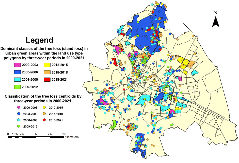
FIGURE 11. Dominant classes of the USL in urban green areas within land use types polygons by 3-year periods in 2000–2021 (GDK-1).
The referred scheme of the dominant USL classes can be a subject of analysis itself: it can be clearly seen that dominant loss took place in the Shevchenkivskyi ward (a city district) of Kharkiv in 2003–2006, which can be explained by both housing and infrastructural network development in this area within the mentioned period (Figure 11). It can be seen from this illustration that, during the period mentioned, there was a loss of UGAs in the Osnovianskyi and Slobidskyi wards of Kharkiv. This trend can be observed in the period of 2006–2009 in Moskovskyi, Nemyshlyanskyi, and Osnoviansky districts. From 2012 to 2015, a similar distribution can be observed in the Kyivskyi ward. Regarding the finalized estimation period (2018–2021), we can see statistically significant USL parcels in the Shevchenkivskyi ward only.
Then, the USL centroids were overlaid on the layer of city wards, as explained in the methodical section above (Figure 12). It can be seen from it that some notable USL occurred within the Osnovianskyi and Shevchenkivskyi wards in 2003–2006 and 2006–2009. The least USL can be objectively seen in territories of the old industrial wards, Industrialnyi and Nemyshlyanskyi, where fewer UGAs were traditionally located. According to this map, we can conclude the minimal loss throughout all wards occurred in 2000–2003.

FIGURE 12. A number of the USL centroids within the administrative districts of Kharkiv in the period of 2000–2021 (GDK-1).
We have already described in the methodical section how we obtained the map of 10 green sub-classes, which correlates with the USL dominant classes. Calculated dominant values of the centroids were transferred into the green LU layer (Figure 13A. This enabled seeing which USL classes were spatially bound to particular LU types of UGAs (farmland, forests, garden, grass, meadow, orchard, park, recreation ground, wood, zoo). This map indicates that the most notable USL parcels occurred within a forest park in the Shevchenkivskyi district. Some territories with the average USL values and green agricultural LU are the peripheral areas of Kyivskyi, Moskovskyi, Nemyshlyanskyi, and Industrialnyi wards. At the same time, there are a few considerable wood areas in the western peripheral locations of the Kholodnohirskyi ward. By the way, one of the most surprising findings is the insignificant USL in this suburban part of the latter ward with few USL parcels related to the period of 2006–2009 (Figure 13A). Spatial comparison of the green LU types with the classified USL centroids proves some conclusions made above already: the largest losses of UGAs were observed in 2003–2006, 2006–2009, and 2015–2018 (Table 2, Figure 8).
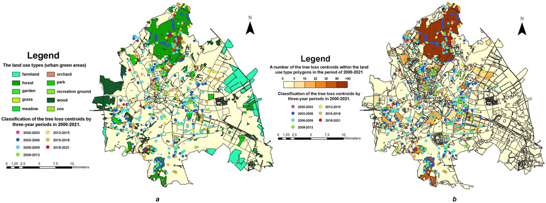
FIGURE 13. (A) The subclasses of the green urban land use associated with the dominant classes of the USL centroids as the point features (GDK-1). (B) Six spatial dominant classes of the urban stand loss in Kharkiv described by the numeric range: 0–>90 and colorized by the unique value methods.
As explained in the methodical section, the results of revealing spatial correlation of urban stand loss with the green land use classes were further reviewed by overlaying the centroid USL layer on other layers displayed in previous maps: dominant USL classes in UGAs with LU type polygons, a number of USL centroids in administrative districts, subclasses of the green urban LU associated with the dominant USL classes (Figures 11–13A). The derivative layer has been colorized by the UVM. As a result, the spatial six dominant USL classes configured the complete urban stand loss distribution within the whole city area. These classes ranged in the UVM legend from the first to the sixth, from left to right, with USL values increasing from lower to higher classes (Figure 13B).
This finalized composite map matches our previous findings made in this research. The greatest loss of the sixth class throughout the whole period of evaluation occurred in the northern part of the city area, where the biggest urban forests (named “Lesopark”) are allocated (Shevchenkivskyi ward). It can be definitely explained by existing environmental conditions—the presence of forest stands in this urban area.
The fifth and the fourth USL spatial classes appeared only fragmentarily to the South and South-West of the “Lesopark” area (again Shevchenkivskyi, but also Kholodnohirskyi wards), which can be explained by the large urban forest presence not far from this location. Few selected parcels of these two classes can be defined in the central part of Kharkiv, in Kyivskyi, Moskovskyi, and Kholodnohirskyi wards. These parcels of relatively high USL values can be caused by another reason compared with those factors determining the sixth class delineation in the northern part. The central part of the city can expose high USL values owing to anthropogenic disturbance of permanent urban infrastructural development in this area. On the contrary, a comparatively large territory of the fourth USL class in the southern part of Novobavarskyi ward should be explained by environmental reasons exclusively (Figure 13B).
Despite being allocated fragmentarily, the third and second USL spatial classes possess almost trice larger areas throughout the city compared to the fifth and fourth classes. The predominance of the classes with lower USL values and total prevalence of the first class with its lowest values throughout the city area prove sustainable long-term dynamics of UGAs in Kharkiv, keeping some balance between their expansion and shrinking, but with minor trending to the latter one.
The latest illustration confirms the USL extremums in 2003–2006, 2006–2009, and 2015–2018 (Figure 13B).
3.4 Analysis of Changes in the Infrastructural Component of Green Areas of Kharkiv
Given the increasing density of urban development, we pay attention to the infrastructural changes in cities. Urban parks are an integral part of the general scheme of city greening. The local authorities focus on the park’s development and infrastructural transformation (Supplementary Material 2A).
The Kharkiv Economic and Social Development Program for 2020 has identified the following priority goals:
• Improving the aesthetic appearance of green facilities and creating appropriate conditions for recreation of the city’s residents, preventing vandalism acts.
• Providing green facilities of the city with the required number of its own produced flower products, introducing energy-saving technologies.
• Meeting the citizens’ cultural needs, creating conditions for the artistic creativity development of the population, conservation of green areas in Kharkiv.
• Improving the environmental condition of soils and green areas
According to the list of investment projects for the facilities construction, the Department of Public Utilities in Kharkiv implemented the following projects at the expense of budget funds in 2020 (Table 3).
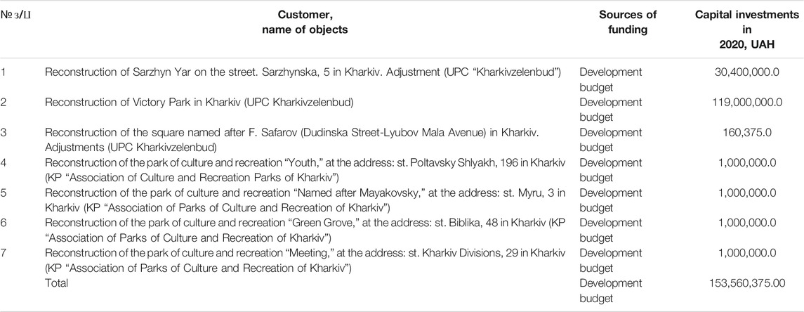
TABLE 3. The number of budget subsidies for the park areas development in the city of Kharkiv in 2020 (About the Program of economic and social development of Kharkiv for 2020, 2021).
In total, in 2020, the city government invested more than 153 million hryvnias in improving Kharkiv’s green areas at the expense of the development budget, which indicates the high interest of the local authorities in developing the city’s green areas and improving its infrastructure. Comparing the project goals of the Kharkiv Development Strategies for 2020 and 2030 (Table 4) regarding the green area’s development, we note that both documents focus on the concept of the “green city” and the city’s integrated green area development.
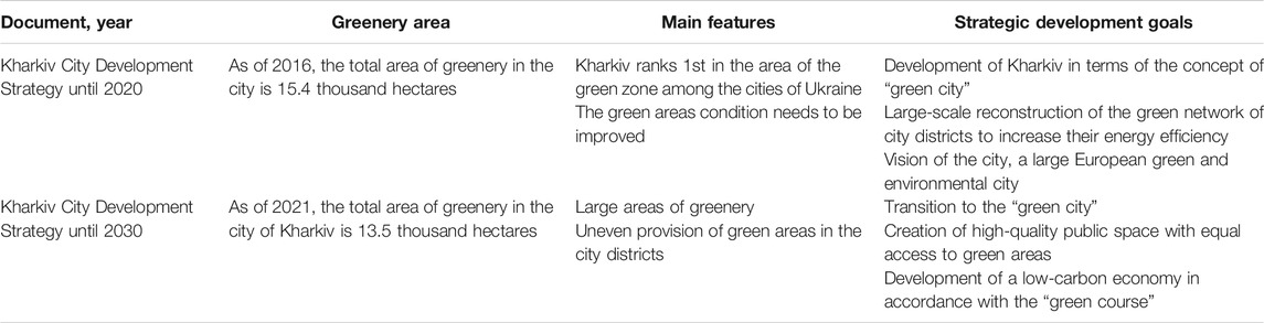
TABLE 4. Perspective development of UGAs of Kharkiv in accordance with the Strategy of development of the city of Kharkiv until 2020 and 2030 (Development Strategy of Kharkiv until 2020, 2021; Development Strategy of Kharkiv until 2030, 2021).
Kharkiv was one of the first cities to launch the Smart City UA project in Ukraine. In October 2021, Kharkiv joined the EBRD Green Cities, which will form an action program to meet the environmental needs and create a more promising and sustainable future for citizens (EBRD Green Cities, 2021; European Bank for Reconstruction and Development, 2021). Under this program, the EBRD and other financial institutions aim to finance the modernization of energy efficiency and infrastructure, transport, lighting and roads, water supply and sanitation, renewable energy sources, solid waste management systems, and so on. Therefore, the memorandum provides a comprehensive analysis of the environmental situation in the city, preparation of measures to improve it, identifying areas of priority investment, and so on through finance, flight loans, and grants (Kharkiv joins Green Cities programme, 2021).
The existing parks, squares, and other UGAs do not interact in such a way and cannot fully affect the environmental corridor. In this regard, the infrastructural and planning public organization “Other Way” proposed the project “Green Network of Kharkiv,” which is the basis of the Development Strategy of Kharkiv until 2030 and supports implementation by the city administration. Kharkiv “Kharkiv joins Green Cities programme, 2021” (Figure 14) is designed as an infrastructural element that should promote the integration of human and nature in the urban system, establish information, and energy exchange within this system; allow city’s residents to interact more closely and feel reunited with the natural environment, provide recreation near the residence and workplaces of citizens (Igor Terekhov spoke, 2021). This is a good opportunity for walking and cycling in the city of various durations on the new routes, which will provide more comfortable moving through the city and somewhat relieve traffic on the city’s main streets due to the “green alternative.” An urgent problem for Kharkiv at the moment is the city streets, which are evaluated mainly based on transport capacity and do not consider the comfort for cyclists or pedestrians, the greening level, which is the first step towards forming a single “green framework” of Kharkiv.
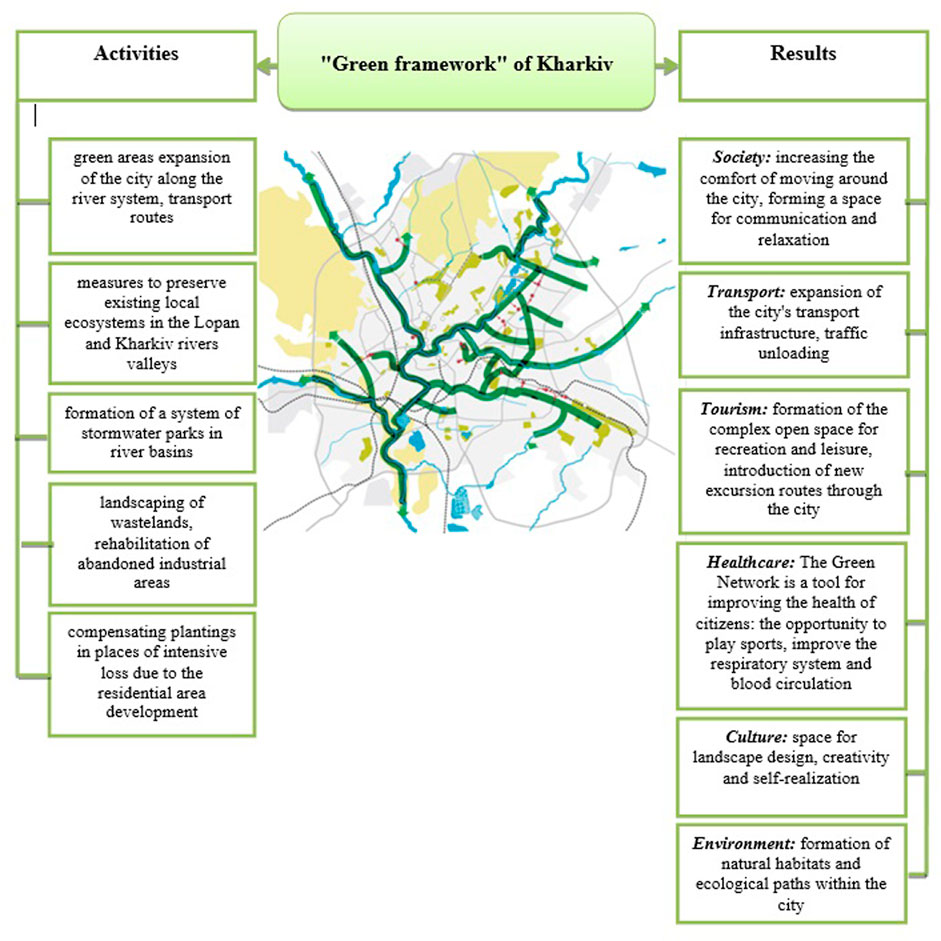
FIGURE 14. “Green framework” of Kharkiv (Official site of Kharkiv City Council, 2021b).
Moreover, forming a “green network” will help expand the city’s socio-cultural function because it will widen the conditions for recreation and communication of citizens. The Green Network can become an open space for art exhibitions, plenaries, and open-air workshops. It is also essential to build transit routes through peripheral parks, increasing their attendance and safety and creating a specific impetus for development. A possible scenario for the transformation of Kharkiv’s green areas is the opening of special-purpose green areas, those located near hospitals, educational institutions, and so on, for all willing vacationers, that is, their transfer to public status. At the same time, it is necessary to consider the socio-psychological side of this issue: the moral and psychological condition of patients, the safety level for students, and so on.
The combination of green areas of the city in a coordinated system provides an opportunity to develop new urban tourist routes. The landscape design techniques provide a wide range of functions and enable these spaces to be green, environmental, and creative. The green network will connect the city road and eliminate the existing dividers (railways, highways, abandoned industrial areas, etc.) by greening the streets and other public spaces.
4 Conclusion
UGAs are a part of the social space and a vital part of the urban landscape, which provides the population’s needs for recreation, quality pastime, psychological pressure and stress reduction, rehabilitation, and so on. Thanks to the green areas, the cities become more comfortable and healthy for living (environmentally friendly). Green areas have significantly expanded their functions in the current conditions of urbanization and gentrification. In addition to sanitary, hygienic, recreational, health, and environmental functions, they are increasingly becoming places of open public spaces to meet society’s needs.
The feature of our study is the green areas of Kharkiv. Kharkiv is the second-largest (by human and economic potential) city in Ukraine, a modern city with a developed infrastructure, a scientific, educational, cultural, and economic center of Ukraine. According to official data, each city inhabitant has about 107 sq.m of green areas at a rate of 50 sq.m, as the WHO determined. Our calculations revealed that one inhabitant of Kharkiv has 35 sq.m of greenery, which exceeds the UN’s standard (30 sq.m). Compared to other Ukrainian cities, Kharkiv has a high supply of green areas concerning the population, and it is the second only to the capital, the city of Kyiv.
The study analyzes the dynamics of the spatial and functional organization of the UGA according to the Master Plans, plan maps, and functional zoning of the city for 1867–2019. The area of Kharkiv has been expanding significantly during its existence, including large suburban areas and, accordingly, green areas. Unfortunately, planning documentation does not provide a clear functional division of the city into appropriate zones. Therefore, it is quite challenging to establish the dynamics of the UGAs with this data segment. Also, this uncertainty makes it possible for construction companies of the city to use certain parts of green areas for housing, which leads to a reduction in the greenery area in the city. The peripheral green areas have become important after the large-scale development of big residential areas during rapid industrial development in remote areas of the city. They provide opportunities for population recreation near living places. Contemporary, the central UGAs are the most comprehensively developed ones while the peripheral UGAs are developing gradually, they are less developed, not so covered by infrastructural components. However, due to the current active housing development and gentrification of the territory, the peripheral UGAs are gradually reduced, requiring urgent measures to expand and improve the infrastructure to perform their recreational functions.
GIS analysis is the most effective tool for establishing the current state and monitoring of the UGA spatial transformations. We used a wide range of GIS platforms and online resources due to the lack of a digital cadastre for any thematic municipal area of Kharkiv. Therefore, the results are unique and scientifically sound. The article presents an original combined approach using urban remote sensing/GIS based on change detection (CD). The primary data of GIS analysis are satellite images for more than 20 years (2000–2020), obtained from EOS Data Analytics (https://eos.com), the most prominent Ukrainian provider of satellite image data. For further image processing, we applied an updated version of the geospatial web services EOS, LandViewer, and Forest Monitoring (using CD technology). We used the Intersect tool of the ArcGIS overlay analysis for seeking factors of the UGAs losses. We have identified such classes of land use as urban forests, parks, and gardens using the extended data of the Open Street Map on the areas’ functional purpose of Kharkiv, available under the QGIS module. The results of the spatial GIS analysis of UGAs of Kharkiv demonstrated that UGAs were not expanding and partially shrinking during the study period. It is accounted for the intensive construction of the residential neighborhoods, primarily peripheral areas, infrastructure development, and expansion of the city transport network. In order to verify the results obtained, we used two alternative GIS projects: “KharkivTimes, 2021” on the open-source QGIS 3.10 software platform combined with Open Street Map vector layers and in the ArcGIS 10.2 interface due to the update from satellite imagery processing. The usage of different approaches to the analysis allowed characterizing configuration and planar parameters of the UGAs for the study period. The greenery area has been reducing over the past 20 years despite many recreation places for the population, such as parks, squares, and gardens.
Thus, the present study revealed that a total stand loss for the Kharkiv region (with forest areas in the suburbs) in the past 20 years (2000–2020) was substantially lower (2.78%) than a corresponding value for a whole country (around 9%). Although, for the city territory, this value was somewhat higher (2.96%), some sustainable trend of UGAs functioning without more or less significant decrease could be proved as existing in a long-term perspective. It was the first research issue addressed. For the second research issue, this study revealed, on the basis of the spatial pattern distribution, two definite factors of stand loss: rapid infrastructural development in the past 20 years and the latent anthropogenic impact. The third and major research issue introduced the original URS/GIS approach to study urban green areas.
The infrastructure of the UGAs is rapidly improved and optimized due to their consolidation and infrastructural transformations. This is due to objective factors such as changes in the functions of these UGAs and the population’s need for better and more comfortable recreation and leisure. Infrastructural changes have a clear socio-demographic direction. UGAs of Kharkiv have undergone significant qualitative and quantitative changes during its existence and development. The question is whether the remaining UGAs can meet the urban residents’ needs and whether urgent action is needed to increase these areas as the forest parks grow dozens and sometimes even hundreds of years. Unfortunately, Master Plans of Kharkiv Development Strategies do not provide comprehensive thematic information on the territories and qualitative characteristics of the UGAs because some outdated methodologies were used for evaluation while these documents were completed. The whole issue can be resolved with the involvement of the urban remote sensing/geoinformation approach only.
Data Availability Statement
The raw data supporting the conclusions of this article will be made available by the authors without undue reservation.
Author Contributions
CM, LN, and SK contributed to the concept and design of the study. CM, LN, SK, and KS developed the program and research structure. CM, LN, and SK justified the systematic approach of the research. SK, TL, LK, and PK organized the database. IT, LK, KK, and PK made the general characteristic of Kharkiv a research area. KK and AV carried out the retrospective analysis of Master Plans. SK and PK performed a spatial-statistical analysis of changes in green areas’ configuration and areal parameters. CM, LN, SK, and KS systematized and interpreted the results of GIS analysis. IT and LK performed an analysis of infrastructural changes in the green areas of the city. LN, KS, and KK carried out a content analysis of regulatory documents in the plan of the territory. CM, LN, SK, and KS justified results and prospects of further research. SK, IT, LK, and KK made graphical and cartographic materials for the research.
Conflict of Interest
The authors declare that the research was conducted in the absence of any commercial or financial relationships that could be construed as a potential conflict of interest.
Publisher’s Note
All claims expressed in this article are solely those of the authors and do not necessarily represent those of their affiliated organizations or those of the publisher, the editors, and the reviewers. Any product that may be evaluated in this article, or claim that may be made by its manufacturer, is not guaranteed or endorsed by the publisher.
Supplementary Material
The Supplementary Material for this article can be found online at: https://www.frontiersin.org/articles/10.3389/fenvs.2022.823129/full#supplementary-material
Abbreviations
AOI, area of interest; GDK, Green Digital Kharkiv (a GIS project); GIS, Geoinformation System; GLAD, Global Land Analysis and Discovery; ID, vector polygon identification number; LU, land use; NDVI, Normalized Difference Vegetation Index; abrOSM, Open Street Map; UGAs, urban green areas; URS, urban remote sensing; USL, urban stand loss; UVM, unique value method.
References
About the Program of economic and social development of Kharkiv for 2020 (2021). About the Program of Economic and Social Development of Kharkiv for 2020. Available at: http://kharkiv.rocks/reestr/685246 (Accessed November 10, 2021).
Anderson, J., HardyRoach, E. J., and Witmer, R. (1976). A Land Use and Land Cover Classification System for Use with Remote Sensor Data. USGS Prof. Paper 964, 1–40.
Austrian military archive (2021). Plan of the City of Kharkiv. Available at: https://uma.lvivcenter.org/uk/collections/133/maps (Accessed November 3, 2021).
Badiu, D. L., Iojă, C. I., PătroescuBreuste, M., BreusteNiță, J. M. R., Artmann, M., Niță, M. R., et al. (2016). Is Urban green Space Per Capita a Valuable Target to Achieve Cities' Sustainability Goals? Romania as a Case Study. Ecol. Indicators 70, 53–66. doi:10.1016/j.ecolind.2016.05.044
Ban, Y., Gong, P., and Giri, C. (2015). Global Land Cover Mapping Using Earth Observation Satellite Data: Recent Progresses and Challenges. ISPRS J. Photogrammetry Remote Sensing 103, 1–6. doi:10.1016/j.isprsjprs.2015.01.001
Bagaliy, D. I., and Miller, D. P. (1993). Album of Ancient Plans of the City of Kharkiv, Photos of its Species and Portraits of its Figures. Appendix to the 2nd volume. Kharkiv: History of Kharkiv.
Banskota, A., Kayastha, N., Falkowski, M. J., Wulder, M. A., Froese, R. E., and White, J. C. (2014). Forest Monitoring Using Landsat Time Series Data: a Review. Can. J. Remote Sensing 40, 362–384. doi:10.1080/07038992.2014.987376
Bartholomé, E., and Belward, A. S. (2005). GLC2000: a New Approach to Global Land Cover Mapping from Earth Observation Data. Int. J. Remote Sensing 26 (9), 1959–1977. doi:10.1080/01431160412331291297
Batool, R., Sarwar, F., and Kanwal, J. (2019). Evaluating Spatial Patterns of Urban Green Spaces in Karachi, Pakistan through Satellite Remote Sensing Techniques. Proc. Pakistan Acad. Sci. A. Phys. Comput. Sci. 56 (1), 45–52.
Botanical Garden of the national importance V.N (2021). Karazin Kharkiv National University. Available at: https://garden-karazin.blogspot.com/(Accessed October 21, 2021).
Cai, Y., Chen, Y., and Tong, C. (2019). Spatiotemporal Evolution of Urban green Space and its Impact on the Urban thermal Environment Based on Remote Sensing Data: A Case Study of Fuzhou City, China. Urban For. Urban Green. 41, 333–343. doi:10.1016/j.ufug.2019.04.012
Chang, H.-S., and Liao, C.-H. (2011). Exploring an Integrated Method for Measuring the Relative Spatial Equity in Public Facilities in the Context of Urban parks. Cities 28 (5), 361–371. doi:10.1016/j.cities.2011.04.002
Chen, A., Yao, X. A., Sun, R., and Chen, L. (2014). Effect of Urban green Patterns on Surface Urban Cool Islands and its Seasonal Variations. Urban For. Urban Green. 13, 646–654. doi:10.1016/j.ufug.2014.07.006
Chen, Y., and Gillieson, D. (2009). Evaluation of Landsat TM Vegetation Indices for Estimating Vegetation Cover on Semi-arid Rangelands: a Case Study from Australia. Can. J. Remote Sensing 35 (5), 435–446. doi:10.5589/m09-037
Cianga, N., and Popescu, A. C. (2013). Green Spaces and Urban Tourism Developmentin Craiova Municipality in Romania. Eur. J. Geogr. 4 (2), 34–45. Available at: http://eurogeojournal.eu/articles/Greenspaces_Tourism_FINAL.pdf.
De Haas, W., HassinkStuiver, J. M., and Stuiver, M. (2021). The Role of Urban Green Space in Promoting Inclusion: Experiences from the Netherlands. Front. Environ. Sci. 9. doi:10.3389/fenvs.2021.618198
De la Barrera, F., Reyes-Paecke, S., and Banzhaf, E. (2016). Indicators for green Spaces in Contrasting Urban Settings. Ecol. Indicators 62, 212–219. doi:10.1016/j.ecolind.2015.10.027
Degórska, B. (2004). Planowanie Terenów Otwartych W Nowej Przestrzeni Miejskiej (Na Przykładzie Strefy Podmiejskiej Warszawy). У: M. Kistowski, Ред. 141–148. doi:10.1016/j.ecolind.2015.10.027Studiaekologiczno-krajobrazowe w programowaniu rozwoju zrównoważonego. Przegląd polskich doświadczeń u progu integracji z Unią Europejską. GdańskAvailable at: http://paek.ukw.edu.pl/wydaw/vol13/degorska_2004.pdf
Development Strategy of Kharkiv until 2020 (2021). Strategy Development City of Kharkov until 2020. Available at: https://www.city.kharkov.ua/assets/files/docs/zakon/strategy2411.pdf (Accessed November 21, 2021).
Development Strategy of Kharkiv until 2030 (2021). Kharkiv Development Strategy 2030. Available at: https://www.city.kharkov.ua/uk/index/strategya-rozvitku-xarkova/strategya-rozvitku-xarkova-2030.html (Accessed November 21, 2021).
Du, H., Cai, W., Xu, Y., WangWang, Z., Wang, Y., and Cai, Y. (2017). Quantifying the Cool Island Effects of Urban green Spaces Using Remote Sensing Data. Urban For. Urban Green. 27, 24–31. doi:10.1016/j.ufug.2017.06.008
Du, M., and Zhang, X. (2020). Urban Greening: A New Paradox of Economic or Social Sustainability? Land Use Policy 92, 104487. doi:10.1016/j.landusepol.2020.104487
EBRD Green Cities (2021). Kharkiv. Available at: https://www.ebrdgreencities.com/our-cities/kharkiv/(Accessed October 6, 2021).
European Bank for Reconstruction and Development (2021). Kharkiv Becomes an EBRD Green City. Available at: https://www.ebrd.com/news/2021/kharkiv-becomes-an-ebrd-green-city-.html (Accessed October 6, 2021).
Famous Kharkiv residents’ sculptures in Shevchenko garden (2021). Sculptures of Famous Kharkiv Residents in the Shevchenko Garden/Kharkiv. Available at: https://li-ga2014.livejournal.com/749297.html (Accessed November 2, 2021).
Franco-Lopez, H., Ek, A. R., and Bauer, M. E. (2001). Estimation and Mapping of Forest Stand Density, Volume, and Cover Type Using the K-Nearest Neighbors Method. Remote Sensing Environ. 77, 251–274. doi:10.1016/S0034-4257(01)00209-7
Garcia-Garcia, M. J., Christien, L., García-Escalona, E., and González-García, C. (2020). Sensitivity of green Spaces to the Process of Urban Planning. Three Case Studies of Madrid (Spain). Cities 100, 102655. doi:10.1016/j.cities.2020.102655
Geoportal of the urban cadastre of the Kharkiv region (2021). Geoportal of the Urban Cadastre of the Kharkiv Region. Available at: http://uga-obl.kharkov.ua/ua/map/planning-schemes#map=11//49.967600705211765//36.27037039106298&&layer=9635585433681688-1,100//2203022170794231611-0,100//2480688532222379983-1,100//2480676013692946364-0,100//2480689652822968281-0,100//2480690616355260385-0,100//2480691422978639850-0,100//2480678457378342853-0,100//1635577588204178460-1 (Accessed November 7, 2021).
Germann-Chiari, C., and Seeland, K. (2004). Are Urban green Spaces Optimally Distributed to Act as Places for Social Integration? Results of a Geographical Information System (GIS) Approach for Urban Forestry Research. For. Pol. Econ. 6, 3–13. doi:10.1016/s1389-9341(02)00067-9
Global Forest Watch (2021). Forest Monitoring Designed for Action. Available at: https://data.globalforestwatch.org/(Accessed September 18, 2021).
Gong, P., Wang, J., Yu, L., Zhao, Y., Zhao, Y., Liang, L., et al. (2013). Finer Resolution Observation and Monitoring of Global Land Cover: First Mapping Results with Landsat TM and ETM+ Data. Int. J. Remote Sensing 34, 2607–2654. doi:10.1080/01431161.2012.748992
Guenat, S., Porras Lopez, G., Mkwambisi, D. D., and Dallimer, M. (2021). Unpacking Stakeholder Perceptions of the Benefits and Challenges Associated with Urban Greenspaces in Sub-saharan Africa. Front. Environ. Sci. 9. doi:10.3389/fenvs.2021.591512
Gupta, K., Kumar, P., Pathan, S. K., and Sharma, K. P. (2012). Urban Neighborhood Green Index - A Measure of green Spaces in Urban Areas. Landscape Urban Plann. 105, 325–335. doi:10.1016/j.landurbplan.2012.01.003
Hansen, M. C., Potapov, P. V., Moore, R., Hancher, M., Turubanova, S. A., Tyukavina, A., et al. (2013). High-Resolution Global Maps of 21st-Century Forest Cover Change. Science 342 (6160), 850–853. doi:10.1126/science.1244693
Huang, Y., Yu, B., Zhou, J., Hu, C., Tan, W., Hu, Z., et al. (2013). Toward Automatic Estimation of Urban green Volume Using Airborne LiDAR Data and High Resolution Remote Sensing Images. Front. Earth Sci. 7 (1), 43–54. doi:10.1007/s11707-012-0339-6
Immitzer, M., Atzberger, C., and Koukal, T. (2012). Tree Species Classification with Random Forest Using Very High Spatial Resolution 8-Band WorldView-2 Satellite Data. Remote Sensing 4 (9), 2661–2693. doi:10.3390/rs4092661
Jalkanen, J., Fabritius, H., Vierikko, K., Moilanen, A., and Toivonen, T. (2020). Analyzing Fair Access to Urban green Areas Using Multimodal Accessibility Measures and Spatial Prioritization. Appl. Geogr. 124, 102320. doi:10.1016/j.apgeog.2020.102320
Jeevalakshmi, D., Narayana Reddy, S., and Manikiam, B. (2016). “Land Cover Classification Based on NDVI Using LANDSAT8 Time Series: A Case Study Tirupati Region,” in Proceedings of International Conference on Communication and Signal Processing (India, 61332–81335. doi:10.1109/iccsp.2016.7754369
Kaplan, G. (2019). Evaluating the Roles of green and Built-Up Areas in Reducing a Surface Urban Heat Island Using Remote Sensing Data. Urbani Izziv. Urbanistični Inštitut Republike Slovenije. 30 (2), 105–112. doi:10.5379/urbani-izziv-en-2019-30-02-004
Kharkiv joins Green Cities programme (2021). Kharkiv Joins Green Cities Programme. Available at: https://en.interfax.com.ua/news/general/772035.html (Accessed October 6, 2021).
Kharkiv substantive provisions general plan 2004 (2021). State Committee of Ukraine on Construction and Architecture. Available at: http://gromada.kh.ua/upload/userfiles/1/genplan.pdf (Accessed November 15, 2021).
Kharkiv Zoo (2021). Animals through the Camera. Available at: https://zoo.kharkov.ua/(Accessed September 15, 2021).
KharkivTimes (2021). Sarzhin Yar's Project Won the Grand Prix. Available at: https://times.kharkiv.ua/uk/2020/09/15/proyekt-sarzhinogo-yaru-vigrav-gran-pri/(Accessed October 21, 2021).
KHARKOVGO (2021a). Central Alley of Victory Park in Kharkov after Reconstruction. Available at: https://kharkovgo.com/places/parki-skvery-sady/tsentralnoj-allei-parka-pobedy-v-harkove-posle-rekonstruktsii/(Accessed October 28, 2021).
KHARKOVGO (2021b). Square "Strelka" in Kharkov: The Most Romantic Square of the City. https://rightpark.com.ua/category/realizovannyie-skeytparki/(Accessed November 12, 2021).
Khoshtaria, T. K., and Chachava, N. T. (2017). The Planning of Urban green Areas and its Protective Importance in Resort Cities (Case of Georgian Resorts). Ann. Agrarian Sci. 15 (2), 217–223. doi:10.1016/j.aasci.2017.05.009
Komarova, N. G. (2006). “Changing the Urban Environment in the Urbanized World: a Contemporary View [Conference Presentation],” in Changes in the Natural Environment at the Turn of the Millennium (Tbilisi-Moscow.
Kostrikov, S., Pudlo, R., Bubnov, D., and Vasiliev, V. (2020b). ELiT, Multifunctional Web-Software for Feature Extraction from 3D LiDAR Point Clouds. Ijgi 9, 650. doi:10.3390/ijgi9110650
Kostrikov, S., Pudlo, R., Bubnov, D., Vasiliev, V., and Fedyay, Y. (2020a). Automated Extraction of Heavyweight and Lightweight Models of Urban Features from LiDAR Point Clouds by Specialized Web-Software. Adv. Sci. Technol. Eng. Syst. J. 5 (6), 72–95. doi:10.25046/aj050609
Kuang, W., and Dou, Y. (20202020). Investigating the Patterns and Dynamics of Urban Green Space in China's 70 Major Cities Using Satellite Remote Sensing. Remote Sensing 12, 1929. doi:10.3390/rs12121929
La Rosa, D. (2014). Accessibility to Greenspaces: GIS Based Indicators for Sustainable Planning in a Dense Urban Context. Ecol. Indicators 42, 122–134. doi:10.1016/j.ecolind.2013.11.011
Lang, S., Moeller, M., Schopfer, E., Jekel, T., Holbling, D., Kloyber, E., et al. (2007). “Quantifying and Qualifying Urban green by Integrating Remote Sensing, GIS, and Social Science Method,” in Use of Landscape Sciences for the Assessment of Environmental Security. Editors I. Petrosillo, F. Muller, K. Jones Bruce, G. Zurlini, K. Krauze, S. Victorovet al. (Netherlands: Springer), 93–105.
Lang, S. (2018). Urban green Valuation Integrating Biophysical and Qualitative Aspects. Eur. J. Remote Sensing 51 (1), 116–131. doi:10.1080/22797254.2017.1409083
Lee, H. J., Ru, J. H., and Yu, Y. G. (2010). Extracting High Quality Thematic Information by Using High-Resolution Satellite Imagery. J. Korean Soc. Geospatial Inf. Syst. 18 (1), 73–81.
Levitska, O. L. (2017). Human-geographical Study of the Planning Structure Transformations in Ivano-Frankivsk-City. [dissertation thesis]. [Kyiv]. Kyiv: Taras Shevchenko National University of Kyiv.
Li, F., Han, L., Liujun, Z., Yinyou, H., and Song, G. (2016). Urban Vegetation Mapping Based on the Hj-1 Ndvi Reconstrction. Int. Arch. Photogramm. Remote Sens. Spat. Inf. Sci. XLI-B8, 867–871. doi:10.5194/isprs-archives-xli-b8-867-2016
Lu, D., Mausel, P., Brondı́zio, E., and Moran, E. (2004). Relationships between forest Stand Parameters and Landsat TM Spectral Responses in the Brazilian Amazon Basin. For. Ecol. Manag. 198, 149–167. doi:10.1016/j.foreco.2004.03.048
Ma, L., Fu, T., and Li, M. (2018). Active Learning for Object-Based Image Classification Using Predefined Training Objects. Int. J. Remote Sensing 39 (9), 2746–2765. doi:10.1080/01431161.2018.1430398
Ma, Q., Su, Y., and Guo, Q. (2017). Comparison of Canopy Cover Estimations from Airborne LiDAR, Aerial Imagery, and Satellite Imagery. IEEE J. Sel. Top. Appl. Earth Observations Remote Sensing 10 (9), 4225–4236. doi:10.1109/JSTARS.2017.2711482
Mäkelä, H., and Pekkarinen, A. (2004). Estimation of forest Stand Volumes by Landsat TM Imagery and Stand-Level Field-Inventory Data. For. Ecol. Manag. 196, 245–255. doi:10.1016/j.foreco.2004.02.049
Master plan of the city of Kharkiv 2019 (2021). Master Plan of Kharkiv 2019. Available at: https://data.gov.ua/dataset/721e73b6-bddc-4a6d-ad5a-a1a5c44a4457/resource/3a2c5bd4-43d9-4b05-bd82-09e2ecebe089 (Accessed November 15, 2021).
Maxim Gorkiy Central park of culture and leisure (2021). About the Park. Available at: https://centralpark.kh.ua/en/o-parke/(Accessed September 28, 2021).
Mezentsev, K. V., Provotar, N. I., Provotar, N. I., and Palchuk, M. V. (2020). Public Spaces through the Lens of Participatory Urban Planning - the Case of Kyiv. Ukr. Geogr. Z. 2, 30–37. doi:10.15407/ugz2020.02.030
Millard, K., and Richardson, M. (2015). On the Importance of Training Data Sample Selection in Random Forest Image Classification: A Case Study in Peatland Ecosystem Mapping. Remote Sensing 7, 8489–8515. doi:10.3390/rs70708489
Morar, C., Dulca, M., and Nagy, G. (2020). Brownfields Regeneration, between Sustainable Urban Development and Cultural Heritage. The Former Military Sites in Oradea, Romania. Jura 8 (1), 75–84. doi:10.37043/JURA.2016.8.1.6
Morar, C., Lukić, T., Basarin, B., Valjarević, A., Vujičić, M., Niemets, L., et al. (2021a). Shaping Sustainable Urban Environments by Addressing the Hydro-Meteorological Factors in Landslide Occurrence: Ciuperca Hill (Oradea, Romania). Ijerph 18 (9), 5022. doi:10.3390/ijerph18095022
Morar, C., Nagy, G., Dulca, M., Boros, L., and Sehida, K. (2019). Aspects Regarding the Military Cultural-Historical Heritage in the City of Oradea (Romania). Annales-anali Za Istrske Mediteranske Studije-series Historia Sociologia (Annals Istrian Mediterr. Stud. Ser. Historia Sociologia) 29 (2), 303–322. doi:10.19233/ASHS.2019.21
Morar, C., Tiba, A., Basarin, B., Vujičić, M., Valjarević, A., Niemets, L., et al. (2021b). Predictors of Changes in Travel Behavior during the COVID-19 Pandemic: The Role of Tourists' Personalities. Ijerph 18 (21), 11169. doi:10.3390/ijerph182111169
National Recreational and Park Association (2021). Improving the Health of Communities for All People through parks, Recreation and Conservation. Available at: https://www.nrpa.org/(Accessed October 2, 2021).
Nazaruk, M., and Zhuk, Yu. (2014). Algorithm of the Socio-Ecological Research of Small Towns. Sci. Notes Ternopil Natl. Pedagogical Univ. Geogr. 36, 8–15.
Neuvonen, M., Sievänen, T., Sievänen, T., Koskela, T., Tönnes, S., and Koskela, T. (2007). Access to green Areas and the Frequency of Visits - A Case Study in Helsinki. Urban For. Urban Green. 6 (4), 235–247. doi:10.1016/j.ufug.2007.05.003
News portal GorodKh (2021). How One of the Favorite Vacation Spots of Kharkiv Residents Has Changed. Available at: https://gx.net.ua/obshhestvo/region/kak-izmenilos-odno-iz-lyubimyh-mest-otdyha-harkovchan-video.html (Accessed October 28, 2021).
Newsroom (2021). Fantasy Park with Glowing Sculptures Opened in Kharkov (Photos). Available at: https://www.newsroom.kh.ua/city/v-harkove-otkryli-fentezi-park-so-svetyashchimisya-skulpturami-foto (Accessed November 7, 2021).
Niemets, K., Sehida, K., Niemets, L., Krainyukov, O., Telebienieva, I., and Kobylin, P. (2018a). “Some Issues of the Formation and Implementation of the Development Strategies of Ukraine’s Regions Taking into Account European Experience,” in Sustainable Economic Development and Application of Innovation Management from Regional Expansion to Global Growth. Editors S. Khalid, and S. Soliman (Seville: International Business Information Management Association), 314–327. Proceedings of the 32nd International Business Information Management Association Conference (IBIMA). Seville, Spain. 15-16 November 2018. Available at: https://ibima.org/accepted-paper/formation-and-implementation-of-the-development-strategies-of-ukraines-regions-in-the-aspect-of-eurointegration/.
Niemets, L., Husieva, N., Suptelo, O., Sehida, K., and Kravchenko, K. (2018b). Research of Brownfields and Greyfields of the City: Theory and Practice. Sustainable Economic Development and Application of Innovation Management from Regional Expansion to Global Growth. Proceedings of the 32nd International Business Information Management Association Conference (IBIMA). Seville, Spain. 15-16 November 2018. 409–435. Available at: https://ibima.org/accepted-paper/research-of-brownfields-and-greyfields-of-the-city-theory-and-practice/.
Niemets, L., Niemets, K., Kravchenko, K., Kliuchko, L., and Kobylin, P. (2019c). “Transition Features to the Polycentric Development of the Region: Technique and Practice of the Research,” in Education Excellence and Innovation Management through Vision 2020, Proceedings of the 33nd International Business Information Management Association Conference (IBIMA). Granada, Spain. 10-11 April 2019. 3093–3101. Available at: https://ibima.org/accepted-paper/transition-features-to-the-policentric-development-of-the-region-technique-and-practice-of-the-research/.
Niemets, L., Suptelo, O., Lohvynova, M., Sehida, K., and Kliuchko, L. (2019a). Post-industrial Development of the City of Kharkiv (Ukraine): Backgrounds and Realities. Vision 2025: Education Excellence and Management of Innovations through Sustainable Economic Competitive Advantage. Proceedings of the 34nd International Business Information Management Association Conference (IBIMA). Madrid, Spain. November, 13-14, 2019. 500–508. Available at: https://ibima.org/accepted-paper/post-industrial-development-of-the-city-of-kharkiv-ukraine-backgrounds-and-realities/.
Niemets, L., Suptelo, O., Lohvynova, M., Sehida, K., and Telebienieva, I. (2019b). “Industrial Heritage as a Composition Af Post-Industrial City (Basic Case Kharkov, Ukraine),” in Education Excellence and Innovation Management through Vision 2020, Proceedings of the 33nd International Business Information Management Association Conference (IBIMA). Granada, Spain. 10-11 April 2019. 3049–3063. Available at: https://ibima.org/accepted-paper/industrial-heritage-as-a-composition-of-post-industrial-city-basic-case-kharkov-ukraine/.
Official site of Kharkiv City Council, Mayor, Executive Committee (2021b). Igor Terekhov Spoke about the Green Framework Project. Available at: https://www.city.kharkov.ua/ru/news/igor-terekhov-rozpoviv-pro-proekt-zeleniy-karkas-47738.html (Accessed November 20, 2021).
Official site of Kharkiv City Council, Mayor, Executive Committee (2021). More than 15 Million People Have Visited Gorky Park. Available at: https://www.city.kharkov.ua/ru/news/park-gorkogo-vidvidali-ponad-15-milyoniv-lyudey-47677.html (Accessed September 21, 2021).
Official site of Kharkiv City Council, Mayor, Executive Committee (2021a). Version for the Visually Impaired. Available at: https://www.city.kharkov.ua/uk/gorodskaya-vlast/ispolnitelnyie-organyi/rajonnyie-administraczii.html (Accessed November 20, 2021).
Pax-Lenney, M., Woodcock, C. E., Macomber, S. A., Gopal, S., and Song, C. (2001). Forest Mapping with a Generalized Classifier and Landsat TM Data. Remote Sensing Environ. 77, 241–250. doi:10.1016/s0034-4257(01)00208-5
Pearse, G. D., Dash, J. P., Persson, H. J., and Watt, M. S. (2018). Comparison of High-Density LiDAR and Satellite Photogrammetry for forest Inventory. ISPRS J. Photogrammetry Remote Sensing 142, 257–267. doi:10.1016/j.isprsjprs.2018.06.006
P. Gamba, and M. Herold (Editors) (2009). Global Mapping of Human Settlement: Experiences, Datasets, and Prospects (Boca Raton, FL, USA: CRC Press).
Potere, D., Schneider, A., Angel, S., and Civco, D. L. (2009). Mapping Urban Areas on a Global Scale: Which of the Eight Maps Now Available Is More Accurate? Int. J. Remote Sensing 30, 6531–6558. doi:10.1080/01431160903121134
Ragab, K. (2014). Quantitative Evaluation of Distribution and Accessibility of Urban green Spaces (Case Study: City of Jeddah). Int. J. Geom. Geosc. 4 (3), 526–535.
Resolution of the Verkhovna Rada of Ukraine (2013). On the Change and Establishment of the Boundaries of Kharkiv, Derhachivsky and Kharkivsky Districts of Kharkiv Region. Bull. Verkhovna Rada (Bvr) 31, 372. Available at: https://zakon.rada.gov.ua/laws/show/5215-VI#Text.
RightPark (2021). Implemented Skate parks. Available at: https://rightpark.com.ua/category/realizovannyie-skeytparki/(Accessed November 15, 2021).
Rostang, O., Gren, A., Feinberg, A., and Pont, M. B. (2021). Promoting Resilient and Healthy Cities for Everyone in an Urban Planning Context by Assessing Green Area Accessibility. Front. Environ. Sci. 23. Nov 2021. doi:10.3389/fbuil.2021.797179
Roy, D. P., Wulder, M. A., Loveland, T. R., C.E., W., Allen, R. G., Anderson, M. C., et al. (2014). Landsat-8: Science and Product Vision for Terrestrial Global Change Research. Remote Sensing Environ. 145, 154–172. doi:10.1016/j.rse.2014.02.001
Schofer, E., and Lang, S. (2006). Finding the Right Shades of Urban Greenery. Available at: https://spie.org/news/0213-finding-the-right-shades-of-urban-greenery (Accessed November 12, 2021).
Schott, J. R., Gerace, A., Woodcock, C. E., Wang, S., Zhu, Z., Wynne, R. H., et al. (2016). The Impact of Improved Signal-To-Noise Ratios on Algorithm Performance: Case Studies for Landsat Class Instruments. Remote Sensing Environ. 185, 37–45. doi:10.1016/j.rse.2016.04.015
Senanayake, I. P., Welivitiya, W. D. D. P., and Nadeeka, P. M. (2013). Urban green Spaces Analysis for Development Planning in Colombo, Sri Lanka, Utilizing THEOS Satellite Imagery - A Remote Sensing and GIS Approach. Urban For. Urban Green. 12, 307–314. doi:10.1016/j.ufug.2013.03.011
Shmyh, R. A., Boyarchuk, V. M., Dobryansʹkyy, I. M., and Barabash, V. M. (2010). Terminological Dictionary-Reference Book on Construction and Architecture. Lviv.
Sholok, I. V. (2014). Comparative Analysis of Large Cities Greening in Ukraine and Europe. Bull. V.N. Karazin Kharkiv Natl. Univ. Ecol. 11, 42–49. Available at: https://periodicals.karazin.ua/ecology/article/view/1624.
Snep, R. P., Voeten, J. G., Mol, G., and Van Hattum, T. (2020). Nature Based Solutions for Urban Resilience: A Distinction between No-Tech, Low-Tech and High-Tech Solutions. Front. Environ. Sci. 8. December 2020. doi:10.3389/fenvs.2020.599060
Strahler, A., Boschetti, L., Foody, G., Fierdi, M., Hansen, M., Herold, M., et al. (2008). Global Land Cover Validation: Recommendations for Evaluation and Accuracy Assessment of Global Land Cover Maps. Ispra: European Comission, Institute for Environment and Sustainability.
StroyObzor (2021). Shevchenko Garden many years Ago. https://stroyobzor.ua/ru/kharkov/news-city/sad-shevchenko-mnogo-let-tomu-nazad-foto (Accessed November 2, 2021).
Successful city (2021). New Urban Park in Kharkiv/. Available at: https://www.successful-city.com/novyj-urban-park-v-harkove/(Accessed November 15, 2021).
Suptelo, O., and Sehida, K. (2020). Factors of Post-Industrial Transformations of Urban Sociogeosystems (Case Kharkiv). Visnyk V.N. Karazin Kharkiv Natl. Univ. Geology. Geogr. Ecol. (53), 194–205. doi:10.26565/2410-7360-2020-53-15
Tigges, J., Lakes, T., and Hostert, P. (2013). Urban Vegetation Classification: Benefits of Multitemporal RapidEye Satellite Data. Remote Sensing Environ. 136, 66–75. doi:10.1016/j.rse.2013.05.001
Tyrväinen, L., Pauleit, S., Seeland, K., and de Vries, S. (2005). “Benefits and Uses of Urban Forests and Trees,” in Urban Forests and Trees. Editors C. C. Konijnendijk, K. Nilsson, T. B. Randrup, and J. Schipperijn (Berlin: Springer-Verlag), 81–114. doi:10.1007/3-540-27684-x_5
Unique Build Сompany (2021). Urban Park on Yuriev’ Boulevard. Available at: https://uniquebuild.com.ua/projects/urban-park-na-bulvare-yureva/(Accessed November 7, 2021).
University of Maryland. Department of Geographical Sciences (2020). Global Forest Change 2000-2020. Data Download. Available at: https://data.globalforestwatch.org/documents/tree-cover-loss/explore (Accessed September 27, 2021).
Valjarević, A., Djekić, T., Stevanović, V., Ivanović, R., and Jandziković, B. (2018). GIS Numerical and Remote Sensing Analyses of forest Changes in the Toplica Region for the Period of 1953-2013. Appl. Geogr. 92, 131–139. doi:10.1016/j.apgeog.2018.01.016
Van Herzele, A., and Wiedemann, T. (2003). A Monitoring Tool for the Provision of Accessible and Attractive Urban green Spaces. Landscape Urban Plann. 63 (2), 109–126. doi:10.1016/S0169-2046(02)00192-5
VGORODE (2021). Gorky Park, Shevchenko Garden, Sarzhin Yar: History of the Kharkiv Parks Emergence. Available at: https://kh.vgorode.ua/news/sobytyia/419679-park-horkoho-sad-shevchenko-sarzhyn-yar-ystoryia-poiavlenyia-kharkovskykh-parkov (Accessed September 21, 2021).
WHO Regional Office for Europe (2017a). Urban Green Space Interventions and Health. Available at: https://www.euro.who.int/__data/assets/pdf_file/0010/337690/FULL-REPORT-for-LLP.pdf (Accessed October 12, 2021).
WHO Regional Office for Europe (2017b). Urban green Spaces: A Brief for Action. Available at: https://www.euro.who.int/__data/assets/pdf_file/0010/342289/Urban-Green-Spaces_EN_WHO_web3.pdf (Accessed September 9, 2021).
Wolff, M., and Haase, D. (2019). Mediating Sustainability and Liveability-Turning Points of Green Space Supply in European Cities. Front. Environ. Sci. 7. doi:10.3389/fenvs.2019.00061
Yang, L., Xian, G., Klaver, J. M., and Deal, B. (2003). Urban Land-Cover Change Detection through Sub-pixel Imperviousness Mapping Using Remotely Sensed Data. Photogramm Eng. Remote Sensing 69, 1003–1010. doi:10.14358/PERS.69.9.1003
Zhang, P., Fan, J., Zhang, P., Zhang, Z., Chen, Z., and Han, L. (20212021). Comparative Study on the Effect of Shape Complexity on the Efficiency of Different Overlay Analysis Algorithms. IEEE Access 9, 1. doi:10.1109/ACCESS.2021.3121753
Zheng, Y. Y., and Wu, G. (2021). Single Shot MultiBox Detector for Urban Forest Tree Detection and Location with High-Resolution Remote Sensing Imagery. Front. Environ. Sci. 12. Available at: https://www.frontiersin.org/articles/10.3389/fenvs.2021.755587/abstract.
Zhou, X., and Wang, Y.-C. (2011). Spatial-temporal Dynamics of Urban green Space in Response to Rapid Urbanization and Greening Policies. Landscape Urban Plann. 100 (3), 268–277. doi:10.1016/j.landurbplan.2010.12.013
Keywords: urban green areas, landscape and recreational zones, spatial and functional organization of the city, functions of urban green areas, GIS, urban remote sensing, Ukraine, Kharkiv
Citation: Morar C, Lukić T, Valjarević A, Niemets L, Kostrikov S, Sehida K, Telebienieva I, Kliuchko L, Kobylin P and Kravchenko K (2022) Spatiotemporal Analysis of Urban Green Areas Using Change Detection: A Case Study of Kharkiv, Ukraine. Front. Environ. Sci. 10:823129. doi: 10.3389/fenvs.2022.823129
Received: 26 November 2021; Accepted: 12 January 2022;
Published: 10 March 2022.
Edited by:
Marco Casazza, University of Salerno, ItalyReviewed by:
Polina Lemenkova, Université libre de Bruxelles, BelgiumNathan Moore, Michigan State University, United States
Copyright © 2022 Morar, Lukić, Valjarević, Niemets, Kostrikov, Sehida, Telebienieva, Kliuchko, Kobylin and Kravchenko. This is an open-access article distributed under the terms of the Creative Commons Attribution License (CC BY). The use, distribution or reproduction in other forums is permitted, provided the original author(s) and the copyright owner(s) are credited and that the original publication in this journal is cited, in accordance with accepted academic practice. No use, distribution or reproduction is permitted which does not comply with these terms.
*Correspondence: Cezar Morar, Y2V6YXJtb3JhckB5YWhvby5jb20=
†These authors have contributed equally to this work and share first authorship