Merging and Downscaling Soil Moisture Data From CMIP6 Projections Using Deep Learning Method

Soil moisture (SM) is an important variable in mediating the land-atmosphere interactions. Earth System Models (ESMs) are the key tools for predicting the response of SM to future climate change. Many ESMs provide outputs for SM; however, the estimated SM accuracy from different ESMs varies geographically as each ESM has its advantages and limitations. This study aimed to develop a merged SM product with improved accuracy and spatial resolution in China for 2015-2100 through data fusion of 25 ESMs with a deep-learning (DL) method. A DL model that can simultaneously perform data fusion and spatial downscaling was used to analyze SM’s future trend in China. Through the model, monthly SM data in four future scenarios (SSP1-2.6, SSP2-4.5, SSP3-7.0, SSP5-8.5) from 2015 to 2100, with a high resolution at 0.25°, was obtained. The evaluation metrics include mean absolute error (MAE), root mean square difference (RMSD), unbiased root mean square difference (ubRMSD), and coefficient of correlation (r). The evaluation results showed that our merged SM product is significantly better than each of the ESMs and the ensemble mean of all ESMs in terms of accuracy and spatial distribution. In the temporal dimension, the merged product is equivalent to the original data after deviation correction and equivalent to reconstructing the fluctuation of the whole series in a high error area. By further analyzing the spatiotemporal patterns of SM with the merged product in China, we found that northeast China will become wetter whereas South China will become drier. Northwest China and the Qinghai-Tibet Plateau would change from wetting to drying under a medium emission scenario. From the temporal scale of the results, the rate of SM variations is accelerated with time in the future under different scenarios. This study demonstrates the feasibility and effectiveness of the proposed procedure for simultaneous data fusion and spatial downscaling to generate improved SM data. The merged data have great practical and scientific implications.

1 Introduction

The land surface hydrological cycle is an important part of the climate system. As an important comprehensive variable in the land-atmosphere interactions, SM has a critical impact on plant growth (Chen et al., 2014) and hydrological processes (Western et al., 2004; Seneviratne et al., 2010). SM affects the climate by changing the surface partitioning of radiation and evapotranspiration (Albergel et al., 2013; Fan et al., 2019). Climate changes also cause an increase in extreme weather events, which make soil moisture (SM) variability increase (Green et al., 2019). According to the Sixth Assessment Report (AR6) working group I of the Intergovernmental Panel on Climate Change (IPCC), the global surface temperature has increased by 1.39°C compared to that before the Industrial Revolution (the average of 1850-1900) (Masson-Delmotte et al., 2021). Global warming could worsen drought conditions in many regions worldwide (Orlowsky and Seneviratne 2013; Wanders et al., 2015; Naumann et al., 2018). Foreseeing the drought in advance and making positive solutions is beneficial to any country. Owing to considerable SM memory (Song et al., 2019), the residence times of SM can be used to predict extreme events (including droughts, heat waves, etc.). The variability of the surface-layer soil moisture (SSM) drops below that of deep-layer soil moisture in dry conditions (Hirschi et al., 2014). SSM is well correlative with deep-layer soil moisture in many cases, and only analyzing SSM lacks little information of deep-layer SM (Qiu et al., 2016). Furthermore, the high-frequency characteristic changes of surface soil moisture are significantly affected by atmospheric changes. Therefore, it is significant to accurately obtain the future change of the temporal and spatial distribution and trend information of SSM.

In recent years, ESMs that considered dynamic, physical, chemical, and biological processes are the key tools for predicting the response of SSM to future climate change. The simulated data by the ESMs provides a research basis for the earth’s response to radiative forcing change (Almazroui et al., 2021). For the aim of solving an ever-expanding range of present scientific questions in the climate change field, the latest Phase Six of the coupled model inter-comparison project (CMIP6) has been launched by the Working Group on Coupled Modelling (WGCM) (Eyring et al., 2016). Compared with Representative Concentration Pathways (RCPs) scenarios in Phase5, CMIP6 is designed with the combination of new emission scenarios driven by Shared Socioeconomic Pathways (SSPs) (van Vuuren et al., 2014) and RCPs, which includes the meaning of future socio-economic development. It is a great development that four SSPs (SSP1-2.6, SSP2-4.5, SSP4-6.0, SSP5-8.5) (Riahi et al., 2017; Fricko et al., 2017; Fujimori et al., 2017; Kriegler et al., 2017) replace respectively the four RCPs (RCP2.6, RCP4.5, RCP6.0, RCP8.5) which are used in CMIP5 and adding another four SSPs (SSP1-1.9, SSP4-3.4, SSP5-3.4OS, SSP3-7.0).

However, the different CMIP6 model products have different uncertainties and sensitivities in each variable which are affected by the future emission scenarios, the algorithms of model physics (Li et al., 2012), and the internal variability of the climate system (Deser et al., 2012; van Pelt et al., 2015; Zhuan et al., 2019). The processes in the earth system are difficult to understand mainly because of their complexity (Zhang and Chen 2021). An extensive assessment of CMIP6 models is presented, and the result shows that no single model performs best in all evaluation methods (Sun and Archibald 2021). So, we need to consider scientifically fusing ESMs products. The traditional fusion method is the ensemble mean, considered a simple and effective data merging technique (Weigel et al., 2008). But this method is easily affected by extreme values which obscure the differences in data so that the simulation advantages of some models in various regions are erased (Bai et al., 2021; Sang et al., 2021). With the development of computer technology, new theories and methods about fusion appear successively. But the application in satellite imageries fusion and remotely sensed products are far more than in ESMs products. Another important issue is that the spatial resolutions of ESMs products are generally low and un-matched. Bilinear interpolation is a commonly used traditional method for solving the first problem. Its calculation process is simple (Crow et al., 2012; Yuan and Quiring, 2017), but the high-frequency signals of the zoomed image are lost. CDF-t (probabilistic downscaling) was used in France and provided good results (Michelangeli et al., 2009). Two statistical downscaling methods, Smooth Support Vector Machine, and Statistical Downscaling Model have a good performance in the upper Hanjiang basin in China (Chen et al., 2012). Systematic mean correction is applied on sea-surface temperature to reduce large biases (Narapusetty et al., 2014). A study over the Tianshan Mountains in China used universal kriging interpolation with stepwise and geographically weighted regression to downscale and correct precipitation data (Lu X. et al., 2019). The methods mentioned above are all processing of a single model and do not make full use of the advantages of each model. Fusion and deviation correction is processed separately and only have good results in a small area.

Advanced algorithms from computer vision can be used to process climate data. Super-Resolution Convolutional Neural Network (Dong et al., 2016), the pioneering work of image super-resolution reconstruction, draws attention to the convolutional neural network of deep-learning (DL), which outperforms the traditional Super-Resolution (SR). Subsequent research (Zhang et al., 2020) also used deep learning methods to achieve SR work for hyperspectral image (HSI). More and more ESMs SSM datasets of different scenarios and history from CMIP6 are available now. SSM data is sufficient to train a DL model for SSM dataset generation. If we regard the climate data of one model as a single-channel image, the color channels of the HSI are equivalent to the multiple different ESMs products. With the idea of HSI SR, we can input the SSM data, which is output by many low-resolution ESMs, and get high-resolution SSM data.

The novelty of this study is that our final output data is downscaled data with the high resolution 0.25° × 0.25°, and merged data that retains the advantages of different ESMs. We have implemented the two functions mentioned above in one model. Therefore, this study uses historical CMIP6 SSM data to train a DL model with fusion and downscaling functions and obtains high-resolution SSM merged data (CMIP6_DL). Then, we verify it with the testing data and compare it with the ensemble mean of CMIP6. Finally, we analyze the trend of SSM changes over China in the future based on CMIP6_DL.

2 Data and Methods

2.1 Study Area

Our study area is China, located in eastern Asia and on the western bank of the Pacific Ocean. We select China since it is a great country in agriculture with a long history and extensive cultivated land area, which contributes significantly to the global agricultural development. China has a land area of 9.6 million square kilometers, ranking third in the world in terms of land area. The land cover in China consists primarily of woodland (29.61%), grassland (27.56%), and agricultural area (13.32%); some less dominant land cover types are residential area (3.36%) and water bodies (3.7%) (http://www.mnr.gov.cn/dt/ywbb/202108/t20210826_2678340.html). Owing to its sheer size, there are complicated geographical conditions and special climate characteristics, especially the continental monsoon climate, which determine that China is a country where droughts frequently occur. The study period ranges from 2015 to 2100, in which we define March-April-May (MAM) as spring, Jun-July-August (JJA) as summer, September-October-November as autumn, and December-January-February as winter with the annual mean and the four seasons.

2.2 Earth System Models Data

This study collects monthly mean simulated SSM from 25 ESMs of CMIP6. This data is openly accessible from https://esgf-node.llnl.gov/projects/cmip6/. All selected SSM is the water mass in the top 10 cm layer (kg/m²). Meanwhile, these are available both in the historical period (1850-2014) and future period (2015-2100) in four scenarios (SSP1-2.6, SSP2-4.5, SSP3-7.0, SSP5-8.5). The brief descriptions of the models we used are shown in Table 1. The raw spatial resolutions of 25 models are different, ranging from 0.7031° to 2.8125°, but mostly close to 2° × 2°. In order to reduce the loss of raw data information, all ESMs data are re-gridded to a uniform resolution of 2° × 2° using bilinear interpolation.

TABLE 1

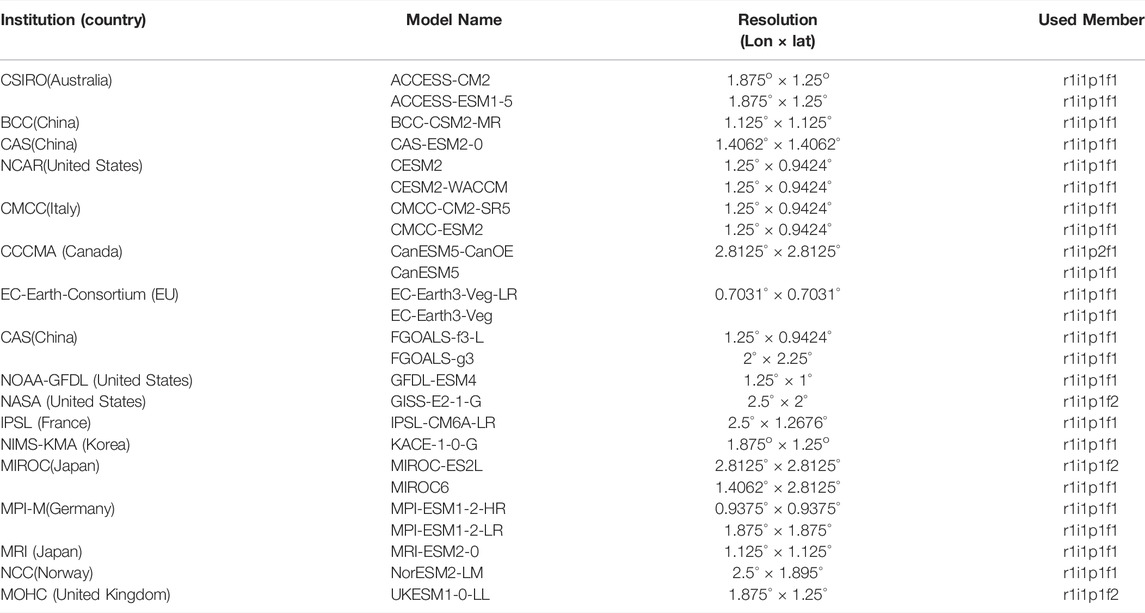
TABLE 1. Details of the 25 CMIP6 models used in this study.

2.3 ERA5-Land Data

Due to improved computing performance in recent years, the European Centre for Medium-Range Weather Forecasts (ECMWF) has produced more detailed global datasets than ever before. The most advanced dataset is the ERA5-Land dataset (Muñoz-Sabater et al., 2021), and the ERA5-Land performed strongly in a SM intercomparison of 18 products with many (826) in situ stations (Beck et al., 2021). Based on the ERA5 reanalysis dataset, the ERA5-Land data is a global numerical reanalysis description of climate data that is generated through multiple data sources into the land surface driving model. Compared to ERA5 and the older ERA-Interim, ERA5-Land is extended back to 1950. This study uses a monthly SSM dataset with a high horizontal resolution of 0.1° × 0.1° from 1950 to 2014. We access it from https://www.ecmwf.int/en/era5-land. The SSM is the water mass in the top 7 cm layer (m³/m³). It has been demonstrated that ERA5-Land has high credibility (Muñoz-Sabater et al., 2021). We select this data to be the reference data to train the model. The greater the factor of downscaling, the greater the error; thus, we chose 8 as a downscaling factor, which made the CMIP6_DL retain the characteristic information of the original models and learn the characteristic information of ERA5-Land. Therefore, we resample ERA5-Land data to 0.25° × 0.25° resolution by bilinear interpolation.

2.4 Methods

2.4.1 Deep-Learning Methods

A neural network called Ynet (Liu, Ganguly, and Dy 2020), which combines image super-resolution techniques and data fusion, is used in this study. We use this DL model to build a relationship between the historical ERA5-Land SSM data and the historical CMIP6 ESMs data. By applying this relationship in the future period, a merged SSM product, which conforms to the characteristics of the ERA5-Land dataset distribution, is developed with improved accuracy and spatial resolution in China for 2015-2100 through data fusion of 25 ESMs.

The model architecture is shown in Figure 1. This architecture includes three parts: the first one is a quasisymmetric structure with skip connections. The input is low-resolution X_ESM. Like RED-Net, this structure tackles the gradient vanishing problem and is regarded as the feature extractor, which captures the abstraction of noisy low-resolution images and outputs the cleaner image. This part consists of 30 convolutional layers and 15 deconvolutional layers. However, the deconvolutional layer may introduce the “checkerboard artifacts” which will reduce the output quality (Odena et al., 2016). The purpose of adding a convolutional layer after each deconvolutional layer is to reduce the checkerboard problem. The second part is the upsampling part, which includes an upsampling layer and two convolutional layers with the same feature depth as the input channel. Similar to the first part, adding the latter two layers is to eliminate the checkerboard effect. Downscaling is the main function of this part. The third part is for fusion. The input of this part contains three datasets: the upsampling part output, auxiliary data and unsampled X_ESM. The auxiliary data is used to help improve the results. It remains the same for different months in the whole training and test period. Concatenating the three datasets calculated by two convolutional layers, the high-resolution merged data is produced. The loss function is calculated as follow:

$L\left(\theta \right)=\frac{1}{N}{\displaystyle \sum _{i=1}^N|\left|f\left(X_i,\theta \right)-Y_i\right|{|}^2}(1)$

where $\theta$ is the network parameters to be optimized. $f\left(X_i,\theta \right)$ is the learnt function. N is the total number of the training dataset samples. X_i is the input and Y_i is the target at location i.

FIGURE 1

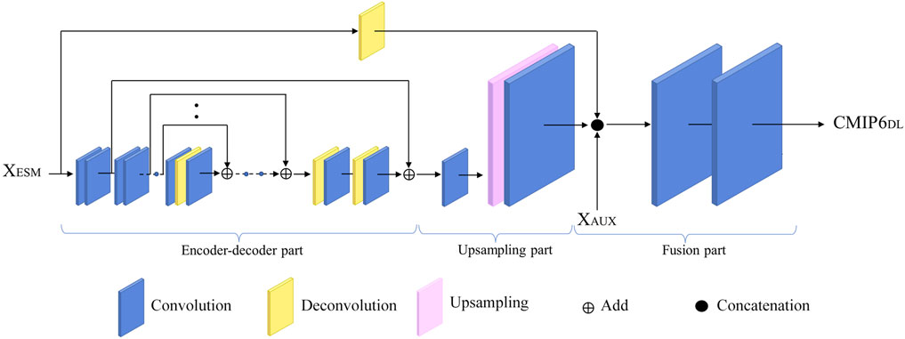
FIGURE 1. Model architecture (Liu et al., 2020).

Since the units of the ESMs data and ERA5-Land data are different and need to be unified, we use the following formula to convert the unit of the ESMs data (kg/m²) into volumetric water content (m³/m³) (Zhu and Shi, 2014).

$\frac{kg}{m^2}\frac{m^3}{1000kg}\frac{1000mm}{1m}\frac{1}{thicknessofthesoillayer\left(mm\right)}\mathrm{=}volumetricwatercontent\left(\raisebox{1ex}{$m^3$}\!\left/ \!\raisebox{-1ex}{$m^3$}\right.\right)$

2.4.2 Evaluation Method

To objectively estimate the performance of CMIP6_DL and know whether it captures the ERA5-Land data distribution characteristics, we use mean absolute error (MAE), root mean square difference (RMSD), unbiased root mean square difference (ubRMSD), and coefficient of correlation (r). The computation formulas are shown as follows:

$MAE=\frac{1}{n}{\displaystyle {\sum }_{i=1}^n\left|S_i\mathrm{-}{E}_i\right|}(2)$

$RMSD\mathrm{=}\sqrt{\frac{\mathrm{1}}{n}{\displaystyle \sum _{i\mathrm{=1}}^n{\left(E_i\mathrm{-}{S}_i\right)}^2}}(3)$

$ubRMSD=\sqrt{\frac{1}{n}{\displaystyle \sum _{i=1}^n{\left[\left(E_i-\overline{E}\right)-\left(S_i-\overline{S}\right)\right]}^2}}(4)$

$r\mathrm{=}\frac{{\displaystyle {\sum }_{i\mathrm{=1}}^n\left[\left(E_i\mathrm{-}\overline{E}\right)\left(S_i\mathrm{-}\overline{S}\right)\right]}}{\sqrt{{\displaystyle {\sum }_{i\mathrm{=1}}^n{\left(E_i\mathrm{-}\overline{E}\right)}^2}}\sqrt{{{\displaystyle {\sum }_{i\mathrm{=1}}^n\left(S_i\mathrm{-}\overline{S}\right)}}^2}}(5)$

In Eqs. 2–5 n is the total number of samples. S_i is the SSM of CMIP6_DL and E_i is the ERA5-Land reanalysis data at location i. $\overline{E}$, $\overline{S}$ represents the average value of CMIP6_DL data and reanalysis data respectively.

2.4.3 Analysis Method

Unlike other climate variables, SSM has a relatively long memory, which refers to the time required for rainfall to dissipate (Seneviratne et al., 2006; McColl et al., 2017). Therefore, the change of SSM can directly reflect the drought situation. However, due to the complexity of the causes of drought and the investigators’ consideration of various factors in the study area, there is no unified mathematical definition of drought (Lloyd-Hughes 2014). Considering the small range of SSM change, it is difficult to see the future change trend directly using the real value of SSM. Therefore, we use a standardized soil index to study the trend of SSM changes in four scenarios. The standardized SM index (SSMI) (Zhou et al., 2019) is calculated as follow:

$SSMI=\frac{SM\mathrm{-}\overline{SM}}{\sigma }(6)$

where in, SM refers to the value of SSM on a certain temporal scale (monthly), $\overline{SM}$ is the mean value of SSM for many years (2015-2100) on this time scale, σ is the standard deviation of SSM for many years on this time scale. SSMI less than 0 means that the SM is less than the normal value, showing a state of SSM deficit. Conversely, the SSM is greater than the normal value, showing a state of SSM surplus. The value of SSMI indicates the degree of deviation from the normal value.

To calculate the SSMI trend, we use the non-parametric Theil-Sen slope (TS) (Sen 1968; Theil 1992) method in this study. It has been widely used in climate studies (Ahmed 2014; Kumar, Tischbein, and Beg 2019). Compared to the traditional method, such as linear regression, this method has high computational efficiency and is insensitive to data outliers (Ohlson and Kim 2015). The formula is as follows:

$TS=mean\left(\frac{x_j\mathrm{-}{x}_i}{j-i}\right)\mathrm{,}\forall j\mathrm{>}i(7)$

where in, mean is the function, x_j and x_i are the data at time j and at the time i in the time series. TS > 0 indicates an upward trend, while TS < 0 indicates a downward trend.

3 Results and Discussion

3.1 Implementation of Deep-Learning Method

We use the re-gridded 25 ESMs data as input X_ESM; thus, the input has 25 channels for SSM data. The original historical ESMs data covers the whole earth, with every month from January 1950 to December 2100 — a total of 1812 months. We focus on China and extract the data within latitude 18°N to 54°N and longitude 71°E to 137°E. There are 18 latitude points and 33 longitude points. The reference target is ERA5-Land data with 18°–53.75°N latitude grid by 0.25°, and 71° to 136.75°E longitude grid by 0.25°. Therefore, the target has a size of 144 × 264 with 1 channel. We divide all historical data into three datasets: the training dataset (1950-1999), the validation dataset (2000-2007) and the testing dataset (2008-2014). The ratio is approximately 8:1:1.

In training the model, we add a land-ocean mask to focus only on the land SSM. We match the 25 ESMs SSM data and the reference data simultaneously as a group and put the groups into the model for training. We apply 100 epochs in the training phase. Because of the limitation of GPU memory constraints, the initial learning rate is 1 × 10^−4, and an epoch iterates one group (that is, the batch-size is set to 1) in the training dataset once. We use the Dropout method (Hinton et al., 2012) during training. Dropout removes certain neurons from the DL model at each training step, which limits the complexity of the network and avoids overfitting. Figure 2 depicts the loss function curves of the training and validation datasets for each epoch. As seen, the loss drops sharply at the beginning of the training process. Subsequently, the loss curves show a fluctuation. The results are as expected with the declining loss. There is convergence after 40 epochs, indicating model stability.

FIGURE 2

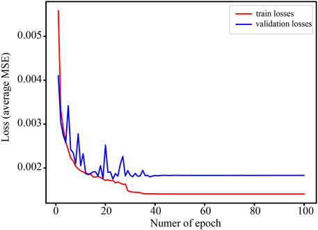
FIGURE 2. Training loss and validation loss curves.

The four evaluation indicators of the model on the testing set are shown in Table 2, where r is the coefficient of spatial correlation. A common fusion method of ESMs data is to compute the ensemble mean of all used ESMs data. Through the evaluation indicators, it can be distinguished which dataset can better capture the characteristics of SSM data distribution. To compare the CMIP6_DL with the ensemble mean of 25 ESMs SSM data under the principle of fairness, we resample 25 ESMs to 0.25° × 0.25° and then calculate the mean of each grid. CMIP6_DL has a better performance than the ensemble mean as shown in Table 2. There is significant improvement by the DL model. We choose spatial correlation as our evaluation method for subsequent spatial change analysis. The SSM spatial distribution is related, but it is fragmented in the dataset generated by the traditional method.

TABLE 2

TABLE 2. MAE, RMSD, ubRMSD, and r (Spatial correlation coefficient) of CMIP6_DL and ensemble mean.

3.2 Evaluation of Fusion Soil Moisture Data

To accurately understand the spatial error distribution, we plot the spatial distribution of MAE, as shown in Figure 3. Figure 3A is the MAE of the testing set of CMIP6_DL and ERA5-Land. The MAE in 70.14% of the study area is less than 0.04, while a few regions of the Qinghai-Tibet Plateau have a large error above 0.06. The Qinghai-Tibetan Plateau is one of the polar regions, and its hydrological cycle is complex (Ullah et al., 2018). The output of the DL model is not satisfactory in eastern Inner Mongolia and Henan-Hebei, with an error of 0.04–0.06. Figure 3B is the MAE of the ensemble mean calculated from traditional approaches and the reference data. MAE is greater than 0.1 in most areas of western and southern China. The error is beyond the acceptable range, so the study’s uncertainty based on the ensemble mean increases. In contrast, the dataset produced by CMIP6_DL is highly reliable.

FIGURE 3

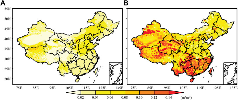
FIGURE 3. MAE discrepancies of monthly mean SSM in the testing dataset (the period of 2008–2014) between (A) CMIP6_DL and ERA5-Land, and (B) ensemble mean and ERA5-Land.

We divide China into four climatic regions: arid zone, semiarid-subhumid zone, humid zone, and Tibetan-Plateau. We select pixels in each region to evaluate the performance in the temporal dimension, as shown in Figure 4. As a whole, we found that the fluctuations of CMIP6_DL and ERA5-Land in the time series are consistent. Observing Figures 4A,B,D, we find that the SSM of the ensemble mean is in phase than the other two datasets but with systematic errors. The minimum values of these three temporal sequences in Figure 4A almost coincide, but the maximum values are not at the same time. The maximum value of CMIP6_DL is between ERA5-Land and ensemble mean but closer to ERA5-Land. It indicates that CMIP6_DL data is equivalent to the original data after deviation correction and expands the range of periodic changes in SSM. Figures 4B,D also illustrate this viewpoint and prove the reliability of the CMIP6_DL data on the temporal scale. The reference data has an SSM anomaly, but the DL model can’t accurately learn this mutation. The original data is limited, so it can be said that the merged data has a “smoothing” effect. Compared with the ensemble mean, the SSM changes of CMIP6_DL in the Qinghai-Tibetan Plateau are tremendous. The main feature of Figure 4C is that the merged data is also equivalent to reconstructing the fluctuation of the whole series in a high error area, which makes the SSM change periodically. The results suggest that the merged data will have good results without anomaly or the data without significant fluctuation. On the contrary, if the mutation of the reference data is irregular, which brings difficulties to the DL model learning, the output data will not perform well.

FIGURE 4

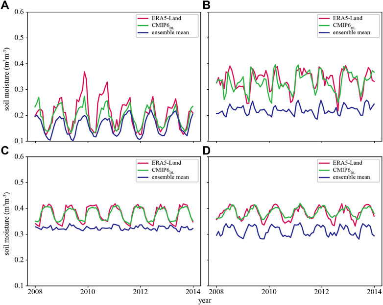
FIGURE 4. Time series of the SSM; each grid is selected from different climatic zoning from 2008 to 2014 for CMIP6_DL. The coordinates of the four grids are (A) 84.5°E, 44.75°N (arid zone) (B) 113.75°E, 39°N (semiarid-subhumid zone) (C) 94°E, 30.25°N (Tibetan-Plateau) (D) 102.25°E, 29.75°N (humid zone).

We use the Normalized Taylor diagram to further evaluate the CMIP6_DL dataset, ESMs datasets, and the reference dataset. Figure 5 shows the distribution of the correlation, ubRMSD, and ratios of standard deviation (STD) for about 28 datasets (including ERA5-Land, CMIP6_DL, the ensemble mean, and 25 ESMs) during 2008–2014. STD is computed as:

$STD=\sqrt{\frac{1}{n}{\displaystyle \sum _{i=1}^n{\left(c_i-\overline{c}\right)}^2}}(7)$

wherein n is the number of all pixels in each dataset; c_i is the specific value of each pixel, and $\overline{c}$ is the average of all pixel values in the current dataset.

FIGURE 5

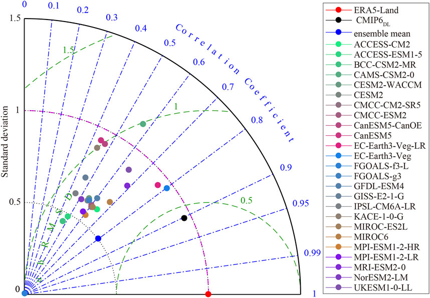
FIGURE 5. Normalized Taylor diagram presenting a comparison of CMIP6_DL dataset with ERA5-Land, the ensemble mean, and 25 models from CMIP6 in 2008–2014. The diagram shows the correlation, ubRMSD, and ratio of the standard deviation.

The overall performance of the CMIP6_DL data, as shown by the selected performance indicators, is better than any other dataset. The products of 25 ESMs show a scattered state with r less than 0.8 and ubRMSD higher than 0.6. There are obvious differences between individual ESMs datasets. Comparing the r and ubRMSD values, the ensemble mean achieves good results following the merged data. Considering the ratio of STD, there is a clear gap between the performance of ensemble mean and merged data, inferring that the amplitude of the ensemble mean is larger than the individual models.

3.3 Future Surface-Layer Soil Moisture Changes Based on CMIP6_DL

3.3.1 Spatial Patterns of Future Surface-Layer Soil Moisture

Based on the 25 ESMs data, we used the trained DL model to fuse the future SSM dataset of the four scenarios (SSP1-2.6, SSP2-4.5, SSP3-7.0, SSP5-8.5). From Figure 6, we can see the spatial distributions of annual change of SSMI under four scenarios (SSP1-2.6, SSP2-4.5, SSP3-7.0, and SSP5-8.5) from 2015 to 2100. From the results, the spatial patterns of SSM trends in the four scenarios are similar; the south is drying while the north is wetting. Under global warming, the arid regions will expand (Huang et al., 2016). Our conclusion confirms the findings of Lu J. et al. (2019) that the average annual SSM shows a large scale drying-wetting trend in China.

FIGURE 6

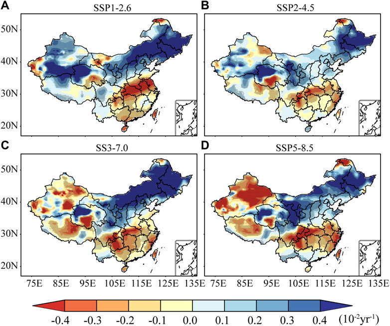
FIGURE 6. Spatial distributions of the annual mean SSMI trend on four future scenarios in the period of 2015–2100 for CMIP6_DL in China. The dots indicate the trend passing the 5% significance test.

The future SSM changes will vary from north to south in China. With 100°E as a dividing line, northwest China and the Qinghai-Tibetan Plateau turn from a wetting trend to a drying trend as the intensity of radiative forcing increases (SSP5-8.5 > SSP3-7.0 > SSP2-4.5 > SSP1-2.6). Under SSP5-8.5, drying becomes more obvious, showing that the environment of this arid region is the vulnerable area affected by continued climate change, which is consistent with Dai (Dai 2013). In Xinjiang, Qinghai and Gansu, under SSP1-2.6, most areas have a palpable wetting trend, and the SSM volumetric water content increases by more than 0.04 (per decade) in southern Xinjiang. However, under SSP5-8.5, the SSM decreases by more than 0.04 (per decade) in nearly half of Xinjiang.

In the east of 100°E, the SSM maintains the drying (wetting) condition in the south (north), but the rate is different under different scenarios. It has become irrefutable that SSM is gradually wetting north of 35°N. The wetting trend is unusually significant and has a wide range, no matter the scenario. Especially under SSP1-2.6 and SSP3-7.0, the wetting trend is greater than 0.05 (per decade). The uneven SSM trend in the northeast is related to historical SSM data because our model is data-driven (Solomatine, See, and Abrahart 2008). In addition to the topographical factors (Chen et al., 2016), local agriculture also affects historical data, such as the rapid reproduction of water-expensive crops and excessive fertilization use (Liu et al., 2015). In southern China, areas with significant drying tendencies have changed. With the increase in radiative forcing, the severe drying trend around 33°N shifts and disperses from north to south to around 30°N. It can be said significant drying trends mainly appear in the Yangtze River basins.

China has a vast land with most of the mainland located in the middle latitudes, which belongs to the northern temperate zone with four distinct seasons. Therefore, it is necessary to analyze the changes of SSM in the future seasons. As shown in Figure 7, the seasonal and annual change trends are spatially different. In general, the SSM in northwest and northeast China is drying or wetting, which is consistent with the average annual SSM (Figure 6), regardless of the season or scenario. In spring, with the low to a high scenario, the area of desiccation increases in China excluding the Qinghai-Tibetan Plateau. Particularly under SSP5-8.5 (Figure 7M), China has the largest drying area, reaching 62.4%. However, unlike Figure 6D, there is a significant wetting trend in the northern Qinghai-Tibetan Plateau. In China, summer is the most significant season of humidification (Du et al., 2020), related to the monsoon climate. Only summer has the largest range of wetting trends in the four scenarios, and the average wetting trend is greater than 0.028 (per decade). With the increase of radiative forcing, the drying rate of northwest China, Qinghai-Tibetan Plateau, Sichuan and Yunnan is rising. In a few areas, SSM decreased by 0.075 per decade. First, the trend of wetting and drying has slowed down slightly. From SSP1-2.6 and SSP2-4.5, we can see that the wetting rate in autumn is much lower than in summer. Under SSP3-7.0 and SSP5-8.5 scenarios, the drying rate of the west of 100°E declines greatly, reaching -0.03. The second change is the acceleration of the wetting area moving westward. Specifically, under SSP3-7.0 and SSP5-8.5, the most wetting areas moved from Heilongjiang, Liaoning, and other places to central Inner Mongolia and Shanxi. Winter is the most significant season of drying out of the four seasons. In the four scenarios, southern China will be drying in winter. The drying trend under SSP5-8.5 is the most severe, with 47.91% of the southern region decreasing by 0.05 every decade. The trend in northwest China is the same as in spring but more pronounced.

FIGURE 7

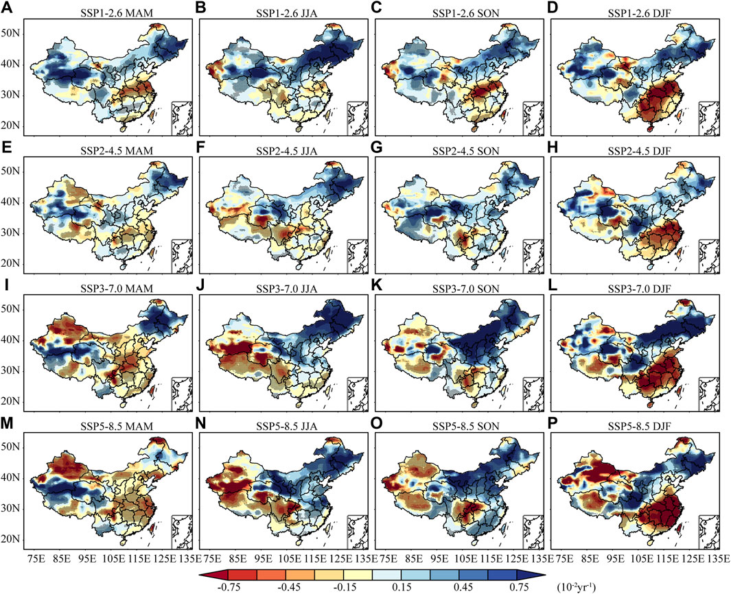
FIGURE 7. Spatial distributions of the annual mean SSMI trend on four future scenarios and seasonal, temporal scale in 2015–2100 for CMIP6_DL in China. The dots indicate the trend passing the 5% significance test.

In summary, SSM will increase in northeast and central China; meanwhile, it will become dry in the south. The SSM trend is affected by radiative forcing in the Qinghai-Tibetan Plateau and northwest China. The wetting and drying trends in different seasons behave differently, but most seasons are projected to dry. In the background of global warming, arid regions will expand in China. The drying rate will become faster in arid regions from lower to higher emission scenarios.

3.3.2 Temporal Change of Future Surface-Layer Soil Moisture

Due to the extended period of the CMIP6_DL data projections, we divide the future period from 2021 into three periods: 2021-2040 (early 21st century), 2041-2070 (middle 21st century), and 2071-2100 (later 21st century). This is convenient for us to analyze the SSM change rate of China on different temporal scales in different periods under four scenarios relative to historical periods, as shown in Figure 8. Because of the differences in SSM between north and south China, they will cancel each other out if they are considered together. Therefore, according to the characteristics of Figure 6, we divide China into north and south regions with 35°N as the boundary and consider them separately. Focusing on changes in SSM, we do not consider the arid regions of the northwest and the Qinghai-Tibetan Plateau; we only investigate the area east of 100°E. Note that since the north has a greater rate of change than the south, the color bars of the two regions are different.

FIGURE 8

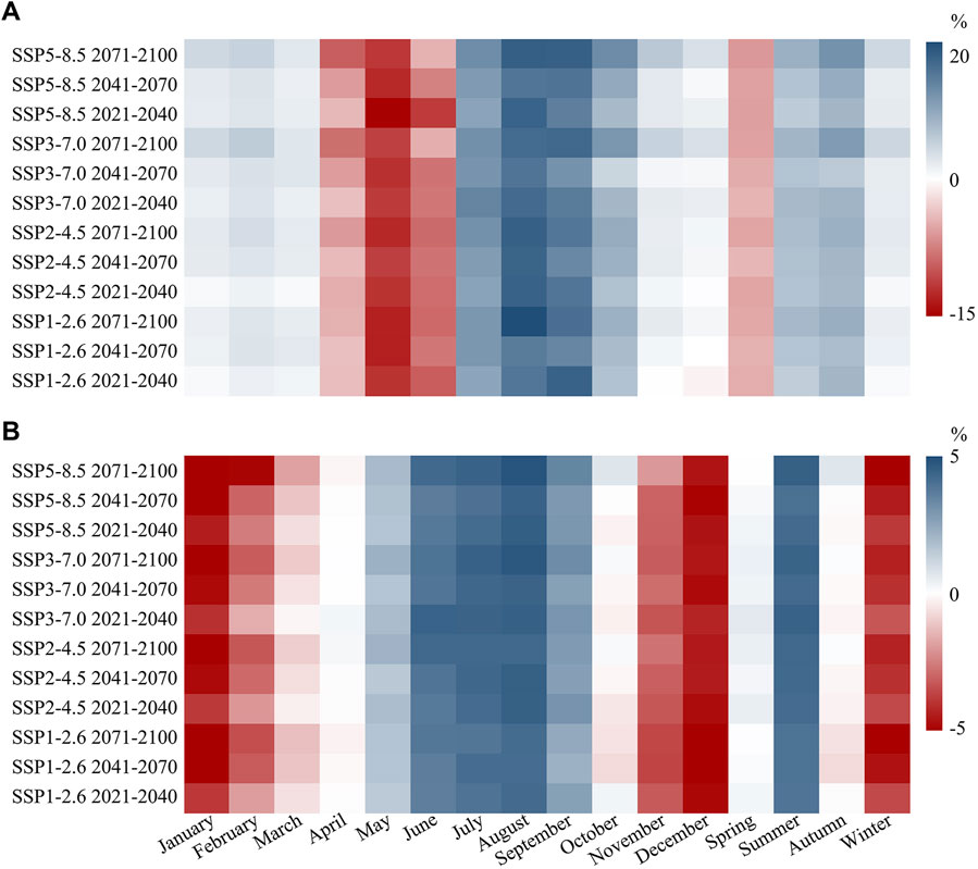
FIGURE 8. The portrait diagram of the SSM change rate of two region in China (A) north of 35°N (B) south of 35°N, in different time scales and future periods relative to the historical period (1995-2014)

From Figure 8, the SSM change rate under each scenario increases with time on the annual scale, regardless of whether it is in the south or north. On the seasonal scale, the north-south differentiation is obvious. The SSM in the north has the highest rate of change in spring and summer, and the rate of change in autumn and winter remains low. Compared with the present, the SSM will increase significantly in summer, and the SSM will be severely dried in spring. This result is not surprising. Spring drought is a common disaster in northern China (Zhang et al., 2018). In recent years, the intensity of summer rainfall has increased, and floods have been frequent in northern China (Sun et al., 2018). Because there is no transition month, this will increase the disparity of SSM surplus and deficit between these two seasons to increase the possibility of disasters (Yu et al., 2021). Therefore, more attention must be paid to quantifying and predicting such environmental changes.

The SSM in the south has the highest rate of change in summer and winter, and there is almost no change in spring and autumn. In winter and summer, the change rate of SSM under each scenario gradually increases, reaching a peak in the later 21st century. Spring and autumn are transitional seasons in the south. SSM in autumn changes from wetting to drying, and the change in spring is from drying to wetting. The SSM change rate varies greatly on a monthly scale. The negative change rate in the northern region reached -14.85% in May, and the change rate in August was as high as 22.36%. The rate of change in the south is generally not as large as in the north. However, there are more months (June, July, August) with a higher rate of change than in the north. Unlike the north, the months with a lower rate of change than in the historical period are December and January, especially in the mid and later 21st century under SSP1-2.6.

In general, under different scenarios, the SSM change rate increases with time in three periods; the seasonal SSM change rate is different between the south and the north. SSM varies greatly from May to August in the north, but SSM varies from December to January and June to August in the south. There are transition months between the positive and negative rate of change in the south, but not in the north.

3.4 Limitations

There are also limitations in this study. First, we did not make full use of the 0.1° × 0.1° high resolution of the ERA5-Land data but used the interpolated 0.25° data. Again, the regional differences of the original data are significant. For example, there is poor model performance in the eastern part of the Inner Mongolia Plain. Regional training may solve this problem (Fan et al., 2021). Finally, because the DL model focuses more on spatial features, temporal information is not fully utilized. Additionally, no separate module can capture this model’s time characteristics. When more ESMs data becomes available, adding these datasets can help reduce errors in future studies.

4 Conclusion

This study used a DL method to produce a high-resolution SSM dataset in China based on CMIP6 ESMs. This method can perform data fusion and data downscaling concurrently. Our merged data significantly improves compared with the individual ESM and ensemble mean data, regardless of the spatial or temporal dimensions. From the evaluation index, the performance of CMIP6_DL exceeds other data in all aspects. The error has been maintained at a low level in mainland China.

We input the ESMs datasets to the model to obtain the SSM dataset under four future scenarios. From the spatiotemporal patterns of the results, the trend of future SSM in China is roughly presented: the northeastern river basins of China become wet, while the Yangtze River basins become dry. With the low to a high scenario, in the east of 100°E, the drying and wetting trends become apparent. In the west of 100°E, the change in the northwest arid region is not just a simple trend enhancement but a change from a wetting trend to a drying trend. From the temporal scale of the results, under different scenarios, the SSM change rate increased with time in the three selected periods. In northern China, the SSM wetting rate will increase significantly in summer and autumn, and the SSM drying rate will increase in spring. Whereas in southern parts of China, the drying trend in winter will increase, and the wetting trend will increase in summer.

Data Availability Statement

The original contributions presented in the study are publicly available. This data can be found here: https://figshare.com/authors/Donghan_Feng/11891447.

Author Contributions

DF: investigation and writing original draft; GW: supervision, discussion and suggestions for data analysis; XW: supervision and editing; SA: writing-reviewing; YH and ZL: discussion and visualization; DH and WU: grammar modification and polishing.

Funding

This study is supported by the National Key Research and Development Program of China (2017YFA0603701) and the National Natural Science Foundation of China (41875094).

Conflict of Interest

The authors declare that the research was conducted in the absence of any commercial or financial relationships that could be construed as a potential conflict of interest.

Publisher’s Note

All claims expressed in this article are solely those of the authors and do not necessarily represent those of their affiliated organizations, or those of the publisher, the editors and the reviewers. Any product that may be evaluated in this article, or claim that may be made by its manufacturer, is not guaranteed or endorsed by the publisher.

References

Ahmed, S. M. (2014). Assessment of Irrigation System Sustainability Using the Theil-Sen Estimator of Slope of Time Series. Sustain. Sci. 9 (3), 293–302. doi:10.1007/s11625-013-0237-1

CrossRef Full Text | Google Scholar

Albergel, C., Dorigo, W., Reichle, R. H., Balsamo, G., de Rosnay, P., Muñoz-Sabater, J., et al. (2013). Skill and Global Trend Analysis of Soil Moisture from Reanalyses and Microwave Remote Sensing. J. Hydrometeorology 14 (4), 1259–1277. doi:10.1175/JHM-D-12-0161.1

CrossRef Full Text | Google Scholar

Almazroui, M., Islam, M. N., Saeed, F., Saeed, S., Ismail, M., Ehsan, M. A., et al. (2021). Projected Changes in Temperature and Precipitation over the United States, Central America, and the Caribbean in CMIP6 GCMs. Earth Syst. Environ. 5 (1), 1–24. doi:10.1007/s41748-021-00199-5

CrossRef Full Text | Google Scholar

Bai, H., Xiao, D., Wang, B., Liu, D. L., Feng, P., and Tang, J. (2021). Multi‐model Ensemble of CMIP6 Projections for Future Extreme Climate Stress on Wheat in the North China plain. Int. J. Climatol 41 (S1), E171–E186. doi:10.1002/joc.6674

CrossRef Full Text | Google Scholar

Beck, H. E., Pan, M., Miralles, D. G., Reichle, R. H., Dorigo, W. A., Hahn, S., et al. (2021). Evaluation of 18 Satellite- And Model-Based Soil Moisture Products Using in Situ Measurements from 826 Sensors. Hydrol. Earth Syst. Sci. 25 (1), 17–40. doi:10.5194/hess-25-17-2021

CrossRef Full Text | Google Scholar

Chen, H., Xu, C.-Y., and Guo, S. (2012). Comparison and Evaluation of Multiple GCMs, Statistical Downscaling and Hydrological Models in the Study of Climate Change Impacts on Runoff. J. Hydrol. 434-435 (435), 36–45. doi:10.1016/j.jhydrol.2012.02.040

CrossRef Full Text | Google Scholar

Chen, T., de Jeu, R. A. M., Liu, Y. Y., van der Werf, G. R., and Dolman, A. J. (2014). Using Satellite Based Soil Moisture to Quantify the Water Driven Variability in NDVI: A Case Study over Mainland Australia. Remote Sensing Environ. 140, 330–338. doi:10.1016/j.rse.2013.08.022

CrossRef Full Text | Google Scholar

Chen, X., Su, Y., Liao, J., Shang, J., Dong, T., Wang, C., et al. (2016). Detecting Significant Decreasing Trends of Land Surface Soil Moisture in Eastern China during the Past Three Decades (1979-2010). J. Geophys. Res. Atmos. 121 (10), 5177–5192. doi:10.1002/2015JD024676

CrossRef Full Text | Google Scholar

Crow, W. T., Kumar, S. V., and Bolten, J. D. (2012). On the Utility of Land Surface Models for Agricultural Drought Monitoring. Hydrol. Earth Syst. Sci. 16 (9), 3451–3460. doi:10.5194/hess-16-3451-2012

CrossRef Full Text | Google Scholar

Dai, A. (2013). Increasing Drought under Global Warming in Observations and Models. Nat. Clim Change 3 (1), 52–58. doi:10.1038/nclimate1633

CrossRef Full Text | Google Scholar

Deser, C., Phillips, A., Bourdette, V., and Teng, H. (2012). Uncertainty in Climate Change Projections: The Role of Internal Variability. Clim. Dyn. 38 (3–4), 527–546. doi:10.1007/s00382-010-0977-x

CrossRef Full Text | Google Scholar

Dong, C., Loy, C. C., and Tang, X. (2016). Accelerating the Super-resolution Convolutional Neural Network. Computer Vis. – ECCV 9906, 391–407. doi:10.1007/978-3-319-46475-6_25

CrossRef Full Text | Google Scholar

Du, Y., Wang, D. Y., Ruan, Y. L., Mo, C. X., and Wang, D. G. (2020). Study on Temporal and Spatial Variation Characteristics of Precipitation Structure in China in Recent 40 Years. Water Power 46 (8), 19–23. doi:10.3969/j.issn.0559-9342.2020.08.005

CrossRef Full Text | Google Scholar

Eyring, V., Bony, S., Meehl, G. A., Senior, C. A., Stevens, B., Stouffer, R. J., et al. (2016). Overview of the Coupled Model Intercomparison Project Phase 6 (CMIP6) Experimental Design and Organization. Geosci. Model. Dev. 9 (5), 1937–1958. doi:10.5194/gmd-9-1937-2016

CrossRef Full Text | Google Scholar

Fan, K., Zhang, Q., Li, J., Chen, D., and Xu, C.-Y. (2021). The Scenario-Based Variations and Causes of Future Surface Soil Moisture across China in the Twenty-First Century. Environ. Res. Lett. 16 (3), 034061. doi:10.1088/1748-9326/abde5e

CrossRef Full Text | Google Scholar

Fan, K., Zhang, Q., Singh, V. P., Sun, P., Song, C., Zhu, X., et al. (2019). Spatiotemporal Impact of Soil Moisture on Air Temperature across the Tibet Plateau. Sci. Total Environ. 649, 1338–1348. doi:10.1016/j.scitotenv.2018.08.399

PubMed Abstract | CrossRef Full Text | Google Scholar

Fricko, O., Havlik, P., Rogelj, J., Klimont, Z., Gusti, M., Johnson, N., et al. (2017). The Marker Quantification of the Shared Socioeconomic Pathway 2: A Middle-Of-The-Road Scenario for the 21st Century. Glob. Environ. Change 42, 251–267. doi:10.1016/j.gloenvcha.2016.06.004

CrossRef Full Text | Google Scholar

Fujimori, S., Hasegawa, T., Masui, T., Takahashi, K., Herran, D. S., Dai, H., et al. (2017). SSP3: AIM Implementation of Shared Socioeconomic Pathways. Glob. Environ. Change 42, 268–283. doi:10.1016/j.gloenvcha.2016.06.009

CrossRef Full Text | Google Scholar

Green, J. K., Seneviratne, S. I., Berg, A. M., Findell, K. L., Hagemann, S., Lawrence, D. M., et al. (2019). Large Influence of Soil Moisture on Long-Term Terrestrial Carbon Uptake. Nature 565 (7740), 476–479. doi:10.1038/s41586-018-0848-x

PubMed Abstract | CrossRef Full Text | Google Scholar

Hinton, G. E., Srivastava, N., Krizhevsky, A., Sutskever, I., and Salakhutdinov, R. (2012). Improving Neural Networks by Preventing Co-adaptation of Feature Detectors. Computer Science 3 (4), 212–223. doi:10.48550/arXiv.1207.0580

CrossRef Full Text | Google Scholar

Hirschi, M., Mueller, B., Dorigo, W., and Seneviratne, S. I. (2014). Using Remotely Sensed Soil Moisture for Land-Atmosphere Coupling Diagnostics: The Role of Surface vs. Root-Zone Soil Moisture Variability. Remote Sensing Environ. 154, 246–252. doi:10.1016/j.rse.2014.08.030

CrossRef Full Text | Google Scholar

Huang, J., Yu, H., Guan, X., Wang, G., and Guo, R. (2016). Accelerated Dryland Expansion under Climate Change. Nat. Clim Change 6 (2), 166–171. doi:10.1038/nclimate2837

CrossRef Full Text | Google Scholar

Kriegler, E., Bauer, N., Popp, A., Humpenöder, F., Leimbach, M., Strefler, J., et al. (2017). Fossil-Fueled Development (SSP5): An Energy and Resource Intensive Scenario for the 21st Century. Glob. Environ. Change 42, 297–315. doi:10.1016/j.gloenvcha.2016.05.015

CrossRef Full Text | Google Scholar

Kumar, N., Tischbein, B., and Beg, M. K. (2019). Multiple Trend Analysis of Rainfall and Temperature for a Monsoon-Dominated Catchment in India. Meteorol. Atmos. Phys. 131 (4), 1019–1033. doi:10.1007/s00703-018-0617-2

CrossRef Full Text | Google Scholar

Li, B., Rodell, M., Zaitchik, B. F., Reichle, R. H., Koster, R. D., and van Dam, T. M. (2012). Assimilation of GRACE Terrestrial Water Storage into a Land Surface Model: Evaluation and Potential Value for Drought Monitoring in Western and Central Europe. J. Hydrol. 446-447 (447), 103–115. doi:10.1016/j.jhydrol.2012.04.035

CrossRef Full Text | Google Scholar

Liu, Y., Ganguly, A. R., and Dy, J. (2020). “Climate Downscaling Using YNet: A Deep Convolutional Network with Skip Connections and Fusion,” in Proceedins of the 26th ACM SIGKDD International Conference on Knowledge Discovery and Data Mining, United States, July 06 2020, 3145–3153. doi:10.1145/3394486.3403366

CrossRef Full Text | Google Scholar

Liu, Y., Pan, Z., Zhuang, Q., Miralles, D. G., Teuling, A. J., Zhang, T., et al. (2015). Agriculture Intensifies Soil Moisture Decline in Northern China. Sci. Rep. 5, 11261. doi:10.1038/srep11261

PubMed Abstract | CrossRef Full Text | Google Scholar

Lloyd-Hughes, B. (2014). The Impracticality of a Universal Drought Definition. Theor. Appl. Climatol 117 (3–4), 607–611. doi:10.1007/s00704-013-1025-7

CrossRef Full Text | Google Scholar

Lu, J., Carbone, G. J., and Grego, J. M. (2019). Uncertainty and Hotspots in 21st Century Projections of Agricultural Drought from CMIP5 Models. Sci. Rep. 9 (1), 4922. doi:10.1038/s41598-019-41196-z

PubMed Abstract | CrossRef Full Text | Google Scholar

Lu, X., Tang, G., Wang, X., Liu, Y., Jia, L., Xie, G., et al. (2019). Correcting GPM IMERG Precipitation Data over the Tianshan Mountains in China. J. Hydrol. 575, 1239–1252. doi:10.1016/j.jhydrol.2019.06.019

CrossRef Full Text | Google Scholar

Masson-Delmotte, V., Zhai, P., Pirani, A., Connors, S. L., Péan, C., Berger, S., et al. (2021). “IPCC, 2021: Summary for Policymakers,” in Climate Change 2021: The Physical Science Basis. Contribution of Working Group I to the Sixth Assessment Report of the Intergovernmental Panel on Climate Change (Cambridge, United States: Cambridge University Press). In Press.

Google Scholar

McColl, K. A., Alemohammad, S. H., Akbar, R., Konings, A. G., Yueh, S., and Entekhabi, D. (2017). The Global Distribution and Dynamics of Surface Soil Moisture. Nat. Geosci 10 (2), 100–104. doi:10.1038/ngeo2868

CrossRef Full Text | Google Scholar

Michelangeli, P.-A., Vrac, M., and Loukos, H. (2009). Probabilistic Downscaling Approaches: Application to Wind Cumulative Distribution Functions. Geophys. Res. Lett. 36 (11), L11708. doi:10.1029/2009GL038401

CrossRef Full Text | Google Scholar

Muñoz-Sabater, J., Dutra, E., Agustí-Panareda, A., Albergel, C., Arduini, G., Balsamo, G., et al. (2021). ERA5-Land: A State-Of-The-Art Global Reanalysis Dataset for Land Applications. Earth Syst. Sci. Data 13 (9), 4349–4383. doi:10.5194/essd-13-4349-2021

CrossRef Full Text | Google Scholar

Narapusetty, B., Stan, C., and Kumar, A. (2014). Bias Correction Methods for Decadal Sea-Surface Temperature Forecasts. Tellus A: Dynamic Meteorology and Oceanography 66 (1), 23681. doi:10.3402/tellusa.v66.23681

CrossRef Full Text | Google Scholar

Naumann, G., Alfieri, L., Wyser, K., Mentaschi, L., Betts, R. A., Carrao, H., et al. (2018). Global Changes in Drought Conditions under Different Levels of Warming. Geophys. Res. Lett. 45 (7), 3285–3296. doi:10.1002/2017GL076521

CrossRef Full Text | Google Scholar

Odena, A., Dumoulin, V., and Olah, C. (2016). Deconvolution and Checkerboard Artifacts. Distill 1, e3. doi:10.23915/distill.00003

CrossRef Full Text | Google Scholar

Ohlson, J. A., and Kim, S. (2015). Linear Valuation without OLS: The Theil-Sen Estimation Approach. Rev. Account. Stud. 20 (1), 395–435. doi:10.1007/s11142-014-9300-0

CrossRef Full Text | Google Scholar

Orlowsky, B., and Seneviratne, S. I. (2013). Elusive Drought: Uncertainty in Observed Trends and Short- and Long-Term CMIP5 Projections. Hydrol. Earth Syst. Sci. 17 (5), 1765–1781. doi:10.5194/hess-17-1765-2013

CrossRef Full Text | Google Scholar

Qiu, J., Crow, W. T., and Nearing, G. S. (2016). The Impact of Vertical Measurement Depth on the Information Content of Soil Moisture for Latent Heat Flux Estimation. J. Hydrometeorol. 17, 2419–2430. doi:10.1175/jhm-d-16-0044.1

CrossRef Full Text | Google Scholar

Riahi, K., van Vuuren, D. P., Kriegler, E., Edmonds, J., Bauer, N., Calvin, K., et al. (2017). The Shared Socioeconomic Pathways and Their Energy, Land Use, and Greenhouse Gas Emissions Implications: An Overview. Glob. Environ. Change 42, 153–168. doi:10.1016/j.gloenvcha.2016.05.009

CrossRef Full Text | Google Scholar

Sang, Y., Ren, H.-L., Shi, X., Xu, X., and Chen, H. (2021). Improvement of Soil Moisture Simulation in Eurasia by the Beijing Climate Center Climate System Model from CMIP5 to CMIP6. Adv. Atmos. Sci. 38 (2), 237–252. doi:10.1007/s00376-020-0167-7

CrossRef Full Text | Google Scholar

Sen, P. K. (1968). Estimates of the Regression Coefficient Based on Kendall's Tau. J. Am. Stat. Assoc. 63 (324), 1379–1389. doi:10.1080/01621459.1968.10480934

CrossRef Full Text | Google Scholar

Seneviratne, S. I., Corti, T., Davin, E. L., Hirschi, M., Jaeger, E. B., Lehner, I., et al. (2010). Investigating Soil Moisture-Climate Interactions in a Changing Climate: A Review. Earth-Science Rev. 99 (3–4), 125–161. doi:10.1016/j.earscirev.2010.02.004

CrossRef Full Text | Google Scholar

Seneviratne, S. I., Koster, R. D., Guo, Z., Dirmeyer, P. A., Kowalczyk, E., Lawrence, D., et al. (2006). Soil Moisture Memory in AGCM Simulations: Analysis of Global Land-Atmosphere Coupling Experiment (GLACE) Data. J. Hydrometeorology 7 (5), 1090–1112. doi:10.1175/jhm533.1

CrossRef Full Text | Google Scholar

Solomatine, D., See, L. M., and Abrahart, R. J. (2008). “Chapter 2 Data-Driven Modelling: Concepts, Approaches and Experiences,” in Practical Hydroinformatics (Germany: Springer-Verlag).

Google Scholar

Song, Y. M., Wang, Z. F., Qi, L. L., and Huang, A. N. (2019). Soil Moisture Memory and its Effect on the Surface Water and Heat Fluxes on Seasonal and Interannual Time Scales. J. Geophys. Res. Atmos. 124, 10730–10741. doi:10.1029/2019JD030893

CrossRef Full Text | Google Scholar

Sun, W., Li, J., Yu, R., and Yuan, W. (2018). Circulation Structures Leading to Propagating and Non-propagating Heavy Summer Rainfall in Central North China. Clim. Dyn. 51 (9–10), 3447–3465. doi:10.1007/s00382-018-4090-x

CrossRef Full Text | Google Scholar

Sun, Z., and Archibald, A. T. (2021). Multi-Stage Ensemble-Learning-Based Model Fusion for Surface Ozone Simulations: A Focus on CMIP6 Models. Environ. Sci. Ecotechnology 8, 100124. doi:10.1016/j.ese.2021.100124

CrossRef Full Text | Google Scholar

Theil, H. (1992). A Rank-Invariant Method of Linear and Polynomial Regression Analysis. Adv. Stud. Theor. Appl. Econom. 23, 345–381. doi:10.1007/978-94-011-2546-8_20

CrossRef Full Text | Google Scholar

Ullah, W., Wang, G., Gao, Z., Hagan, D. F. T., and Lou, D. (2018). Comparisons of Remote Sensing and Reanalysis Soil Moisture Products over the Tibetan Plateau, China. Cold Regions Sci. Technol. 146, 110–121. doi:10.1016/j.coldregions.2017.12.003

CrossRef Full Text | Google Scholar

van Pelt, S. C., Beersma, J. J., Buishand, T. A., van den Hurk, B. J. J. M., and Schellekens, J. (2015). Uncertainty in the Future Change of Extreme Precipitation over the Rhine Basin: The Role of Internal Climate Variability. Clim. Dyn. 44 (7–8), 1789–1800. doi:10.1007/s00382-014-2312-4

CrossRef Full Text | Google Scholar

van Vuuren, D. P., Kriegler, E., O’Neill, B. C., Ebi, K. L., Riahi, K., Carter, T. R., et al. (2014). A New Scenario Framework for Climate Change Research: Scenario Matrix Architecture. Climatic Change 122 (3), 373–386. doi:10.1007/s10584-013-0906-1

CrossRef Full Text | Google Scholar

Wanders, N., Wada, Y., and van Lanen, H. A. J. (2015). Global Hydrological Droughts in the 21st Century under a Changing Hydrological Regime. Earth Syst. Dynam. 6 (1), 1–15. doi:10.5194/esd-6-1-2015

CrossRef Full Text | Google Scholar

Weigel, A. P., Liniger, M. A., and Appenzeller, C. (2008). Can Multi-Model Combination Really Enhance the Prediction Skill of Probabilistic Ensemble Forecasts? Q.J.R. Meteorol. Soc. 134 (630), 241–260. doi:10.1002/qj.210

CrossRef Full Text | Google Scholar

Western, A. W., Zhou, S.-L., Grayson, R. B., McMahon, T. A., Blöschl, G., and Wilson, D. J. (2004). Spatial Correlation of Soil Moisture in Small Catchments and its Relationship to Dominant Spatial Hydrological Processes. J. Hydrol. 286 (1–4), 113–134. doi:10.1016/j.jhydrol.2003.09.014

CrossRef Full Text | Google Scholar

Yu, L. H., Xie, W. S., Xiong, S., Zhang, X., Xing, C., and Hu, S. S. (2021). Characteristics of Drought and Flood Based on SPEI and its Impact on Wheat Yield in Chuzhou of Anhui Province. J. Arid Meteorology 39 (5), 742–749. doi:10.11755/j.issn.1006-7639(2021)-05-0742

CrossRef Full Text | Google Scholar

Yuan, S., and Quiring, S. M. (2017). Evaluation of Soil Moisture in CMIP5 Simulations over the Contiguous United States Using In Situ and Satellite Observations. Hydrol. Earth Syst. Sci. 21 (4), 2203–2218. doi:10.5194/hess-21-2203-2017

CrossRef Full Text | Google Scholar

Zhang, L., Nie, J., Wei, W., Zhang, Y., Liao, S., and Shao, L. (2020). “Unsupervised Adaptation Learning for Hyperspectral Imagery Super-resolution,” in IEEE/CVF Conference on Computer Vision and Pattern Recognition (CVPR),Seattle, WA, June 2020, 3070–3079. doi:10.1109/CVPR42600.2020.00314

CrossRef Full Text | Google Scholar

Zhang, L., Wu, P., Zhou, T., and Xiao, C. (2018). ENSO Transition from La Niña to El Niño Drives Prolonged Spring-Summer Drought over North China. J. Clim. 31 (9), 3509–3523. doi:10.1175/JCLI-D-17-0440.1

CrossRef Full Text | Google Scholar

Zhang, S., and Chen, J. (2021). Uncertainty in Projection of Climate Extremes: A Comparison of CMIP5 and CMIP6. J. Meteorol. Res. 35 (4), 646–662. doi:10.1007/s13351-021-1012-3

CrossRef Full Text | Google Scholar

Zhou, H., Wu, J., Li, X., Liu, L., Yang, J., and Han, X. (2019). Suitability of Assimilatec Data-Based Standardized Soil Moisture Index for Argricultural Drought Monitoring. Acta Ecologica Sinica 39 (6), 2191–2202. doi:10.5846/stxb201801190153

CrossRef Full Text | Google Scholar

Zhu, Z., and Shi, C. X. (2014). Simulation and Evaluation of CLDAS and GLDAS Soil Moisture Data in China. Sci. Technol. Eng. 14 (32), 138–144. doi:10.3969/j.issn.1671-1815.2014.32.028

CrossRef Full Text | Google Scholar

Zhuan, M., Chen, J., Xu, C. Y., Zhao, C., Xiong, L., and Liu, P. (2019). A Method for Investigating the Relative Importance of Three Components in Overall Uncertainty of Climate Projections. Int. J. Climatol 39 (4), 1853–1871. doi:10.1002/joc.5920

CrossRef Full Text | Google Scholar