 Mathew J. Lipson
 Negin Nazarian
 Melissa A. Hart
 Kerry A. Nice
 Brooke Conroy
- 1ARC Centre of Excellence for Climate System Science, University of New South Wales, Sydney, NSW, Australia
- 2ARC Centre of Excellence for Climate Extremes, University of New South Wales, Sydney, NSW, Australia
- 3School of Built Environment, University of New South Wales, Sydney, NSW, Australia
- 4City Futures Research Centre, University of New South Wales, Sydney, NSW, Australia
- 5Transportation, Health and Urban Design Research Lab, Faculty of Architecture, Building, and Planning, University of Melbourne, Melbourne, VIC, Australia
- 6School of Earth and Environmental Sciences, University of Wollongong, Wollongong, NSW, Australia
In urban climate studies, datasets used to describe urban characteristics have traditionally taken a class-based approach, whereby urban areas are classified into a limited number of typologies with a resulting loss of fidelity. New datasets are becoming increasingly available that describe the three-dimensional structure of cities at sub-metre micro-scale resolutions, resolving individual buildings and trees across entire continents. These datasets can be used to accurately determine local characteristics without relying on classes, but their direct use in numerical weather and climate modelling has been limited by their availability, and because they require processing to conform to the required inputs of climate models. Here, we process building-resolving datasets across large geographical extents to derive city-descriptive parameters suitable as common model inputs at resolutions more appropriate for local or meso-scale modelling. These parameter values are then compared with the ranges obtained through the class-based Local Climate Zone framework. Results are presented for two case studies, Sydney and Melbourne, Australia, as open access data tables for integration into urban climate models, as well as codes for processing high-resolution and three-dimensional urban datasets. We also provide an open access 300 m resolution building morphology and surface cover dataset for the Sydney metropolitan region (approximately 5,000 square kilometres). The use of building resolving data to derive model inputs at the grid scale better captures the distinct heterogenetic characteristics of urban form and fabric compared with class-based approaches, leading to a more accurate representation of cities in climate models. As consistent building-resolving datasets become available over larger geographical extents, we expect bottom-up approaches to replace top-down class-based frameworks.
1 Introduction
A transformation is underway in how urban form and fabric are described for urban climate modelling and observation studies. For the last 50 years, datasets used in urban environment or climate studies have typically described urban areas using types or classes in a “top-down” approach, whereby regions of a city, and sometimes surrounds, are classified based on a limited number of urban surface and land-use characteristics (e.g., Masson et al., 2003; Jackson et al., 2010; Stewart and Oke, 2012; Demuzere et al., 2020). In more recent years, very high resolution (sub-metre) urban datasets have become increasingly available that resolve the characteristics of individual buildings and trees over entire cities, regions and continents (PSMA Australia, 2020; Biljecki et al., 2021; Sirko et al., 2021).
These new building-resolving datasets are transforming the way cities can be represented in urban climate models, as spatial dataset parameters are no longer tied to a class type but can be defined for each model grid at any resolution from the “bottom-up” (Figure 1). Where available, these new datasets can be used to produce direct inputs for climate modelling studies at the grid level, or to inform locally appropriate parameter choices in traditional class approaches. The transition to a bottom-up approach, however, is ongoing as many regions do not have access to this urban element-resolving data, and many urban climate models are designed to rely on a class approach when defining urban area characteristics (Masson et al., 2020).
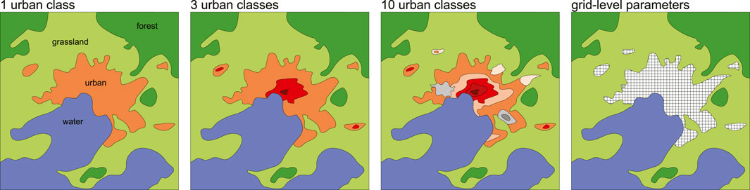
FIGURE 1. Schematic of the transformation of city-descriptive data from top-down derived urban classifications (ranging from a single urban class to the ten urban classes defined by the LCZ system, left to right) to gridded model input of parameters (right) over large geographical areas, that are derived bottom-up from building and tree resolving datasets.
Enhanced accuracy in the representation of urban areas in climate modelling is vital. Cities experience the dual burden of global warming from increased greenhouse gas emissions, and localised warming due to urbanization. This urban heat differs not only from the non-urbanised surrounds but also spatially within a city due to differences in urban density and surfaces. To fully understand the interaction between climates of cities and assess the role of both current and future urbanization in urban climate challenges, it is important for this intra-urban variability to be captured when modelling a city’s climate (Martilli et al., 2020; Potgieter et al., 2021).
Accurate representation of urban areas requires description of four categories of features in both the urbanized areas and surrounds: a) form (urban and vegetated morphology), fabric (materials and surface cover), function (land use and anthropogenic effects), and regional geographic factors (topography and distance from water). Due to computational costs, however, mesoscale models are unable to resolve all urban features while modelling atmospheric processes spanning the entire region. Instead, urban canopy models are defined that assume simplified building geometry in a “building-averaged” approach. The most common geometrical assumptions used in urban models are bulk (1-dimensional), canyon (2-dimensional) or block array (3-dimensional) (Nazarian, 2022). Different modelling assumptions then require different types of morphological and surface cover inputs (outlined in Table 1), further distinguished by the representation of sub-models for vegetation impact and/or thermal comfort characteristics within the street canopy. Accurate urban descriptions are of even greater importance with local and micro-scaled modelling (at sub 10 m resolutions) and in three dimensions, with models such as PALM (Fröhlich and Matzarakis, 2020), ENVI-met (Bruse, 1999), VTUF-3D (Nice et al., 2018), and SOLWEIG/UMEP (Lindberg et al., 2018), as the improved model input can result in more realistic output.
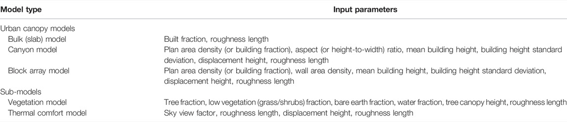
TABLE 1. City-descriptive parameters for various modelling purposes.
Historically, urban areas have been captured in models via land use classification. This is often done by just one urban land type, where different urban regions are represented with a constant set of parameters. Single class approaches have been used in both global models (if urban areas are represented) (Li et al., 2016; Katzfey et al., 2020) and in mesoscale models (Argüeso et al., 2014). Moving beyond one urban land-use class, cities in global or mesoscale models have also been classified on levels of urban density (Ma et al., 2018; Oleson and Feddema, 2020) or by dividing urban areas into different categories such as residential, commercial, and industrial (Chen et al., 2016). These methods provide information on urban form and/or function but fidelity is limited by the number of defined classes.
In a key development, Stewart and Oke (2012) proposed Local Climate Zones (LCZ). LCZs classify city form, fabric, and function into 10 urban classes, and non-urban land cover types into seven classes. The primary motivation for developing LCZs was to improve the description of sites in observational studies in a move away from the historical urban-rural differentiation when investigating urban heat. The classification has been widely used to determine appropriate urban and rural sites for traditional urban heat island intensity calculations (Siu and Hart, 2013) and to explore variability in intra-urban air temperatures in observation studies (Núñez-Peiró et al., 2021; Potgieter et al., 2021).
LCZs have also become commonly used in urban climate modelling, with LCZ classes being integrated into urban land cover classification in mesoscale models (Brousse et al., 2016; Zonato et al., 2020). World Urban Database and Access Portal Tools (Ching et al., 2018), a community led initiative to collect worldwide data on urban form, fabric and function, at its lowest level of detail produces LCZ maps of cities and their surrounding areas. The maps are produced via users classifying small subsections of a city as training data, which are then used in machine learning algorithms to classify the entire region of interest. More recently, WUDAPT workflows have been streamlined into open, online services (e.g., the LCZ Generator; Demuzere et al., 2021).
A limitation of the LCZ approach in the context of numerical modelling is that LCZ parameters are provided as a range of values with substantial overlap between classes, while urban canopy models typically accept explicitly defined values. Common methods of dealing with these challenges include using the midpoints of the LCZ range proposed in Stewart and Oke (2012) for each LCZ used (Mughal et al., 2019), or setting the parameters for LCZ ranges using additional datasets that provide local knowledge (Hirsch et al., 2021).
These traditional top-down approaches, although useful for widespread analyses where data may be lacking, have limitations in that there is often a level of local knowledge or estimation required when setting parameter values, and that outputs are not likely to be consistent between different users and regions. New urban datasets are emerging that directly characterize the 3D urban form produced via methods such as LiDAR and aerial photography observations. Among these high-resolution datasets is the emergence of 3D building models that provide comprehensive representation of built environments in cities across large geographical extents (Biljecki et al., 2016; Biljecki et al., 2021). These novel datasets allow a bottom-up assessment of parameters required to accurately represent intra-urban variability in urban form in climate models, and some have been used to configure models at city-scales (e.g., Simón-Moral et al., 2020). Potential datasets include very high-resolution (∼1 m) surface cover data, three-dimensional building or tree data, as well as incidental and public domain data that can be extracted from social media or the web, contributing to a multi-disciplinary approach to urban climate research, i.e., urban climate informatics (Middel et al., 2022). Coverage of suitable bottom-up datasets, especially at a global scale, remains a challenge. Global datasets of high-resolution impervious surface maps (Zhang et al., 2020; Sun et al., 2022) or urban dwellings (e.g., the Global Urban Footprint (GUF) (Esch et al., 2012)) are becoming available but lack important characteristics such as land cover types and feature heights. The Copernicus Land Monitoring Service updates the CORINE Land Cover dataset (Büttner, 2014) providing 27 land cover classes at 6-year intervals but only provides coverage of Europe (39 countries). Some promising global morphology datasets derived from satellite data have begun to be reported (Esch et al., 2022), but as of writing are not yet publicly available.
In this paper, we use high-resolution, element-resolving datasets to 1) create maps which define actual urban form through the different urban parameters necessary for urban climate models, gridded to appropriate scales, without the fidelity limitations of class approaches and 2) improve traditional class-based approach parameter choices with local data. We use the Australian cities of Sydney and Melbourne as case studies and describe how to extract precise and localized ranges of model parameters using the continental-scale Geoscape datasets (PSMA Australia, 2020) of individual building geometry with ∼1 m accuracy (Geoscape Buildings v2.0, 2020), 2 m land surface (Geoscape Surface Cover v1.6, 2020) and tree characteristics (Geoscape Trees v1.6, 2020). These parameter values are then compared with those calculated by the LCZ method (Stewart and Oke, 2012) via a distribution assessment and presented as data tables for integration into urban climate models.
2 Materials and Methods
This section details the city-descriptive data used and processed in this analysis. Two data sources are considered: 1) Local Climate Zone (LCZ) maps which represent a top-down approach for characterizing urban neighbourhoods based on local urban form, and 2) the Geoscape datasets that represent the bottom-up method for detailing three-dimensional form at the level of individual buildings and trees. While the LCZ maps are defined and developed at local scales, building-resolving datasets require reprocessing to resolutions suitable for observation and modelling studies. The list of urban parameters that are available through processing both data sources are included in Table 2. These parameters cover a range of inputs required by urban climate models pertaining to surface cover, morphology, canopy attribute, and thermal attributes (Table 1).
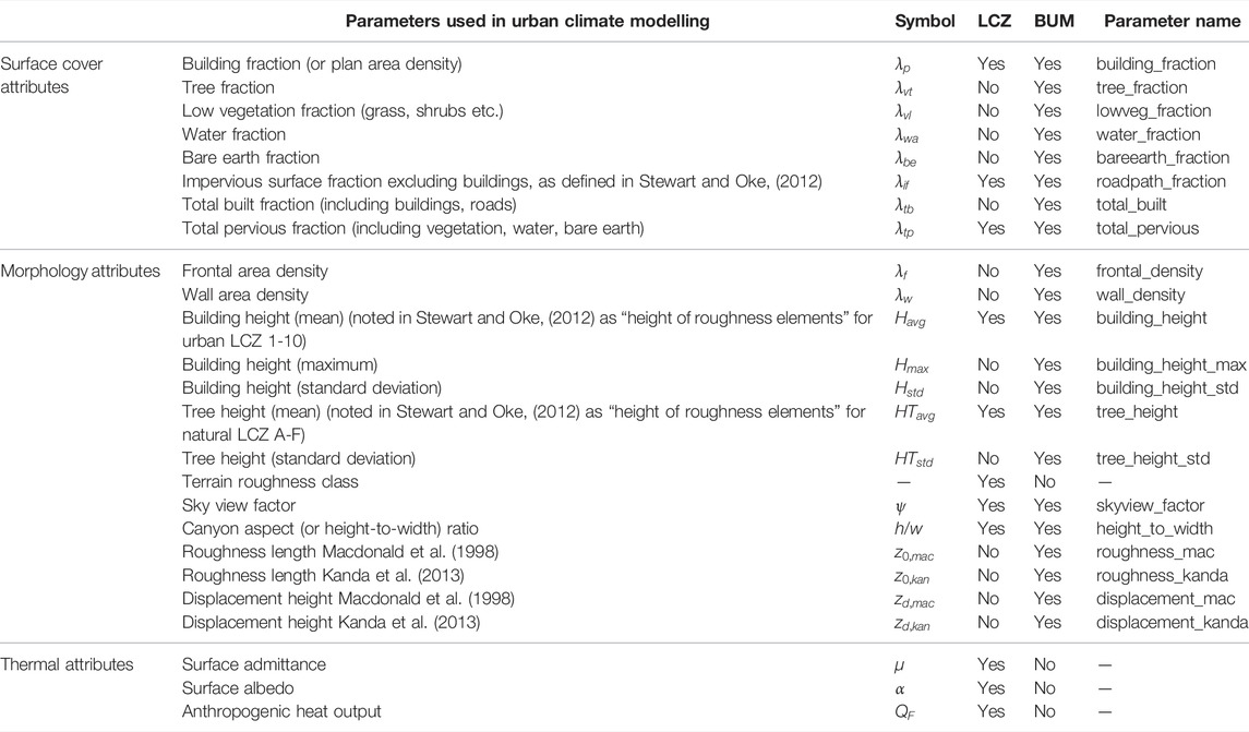
TABLE 2. List and symbols of urban parameters available through LCZ maps and our bottom-up method (BUM) using building and tree resolving datasets. The name of each parameter in the final processed dataset is also shown.
Sydney and Melbourne greater regions are selected for this analysis as they represent the largest metropolitan areas in Australia with a population of 5.4 and 5.1 million, respectively (census data obtained by Australian Bureau of Statistics in June 2020). The climate subtype of Sydney and Melbourne is classified as temperate with warm summers and cool winters, according to the modified Köppen-Geiger classification system used by the Australian Bureau of Meteorology and based on a standard 30-year climatology (1961–1990) (Bureau of Meteorology, 2021).
2.1 Local Climate Zone Datasets
To provide a standardized landscape classification for both Sydney and Melbourne, maps of local climate zones (LCZs) at 100 m resolution are obtained from the LCZ Generator tool (Demuzere et al., 2021) as part of the WUDAPT initiative (Bechtel et al., 2015; Ching et al., 2018). The LCZ Generator is available as a web-based platform that enables the LCZ mapping of global cities using freely available satellite imagery and machine learning algorithms. The LCZ classification requires valid training areas (obtained using local insight) as input parameters and uses an automated cross-validation approach (Bechtel et al., 2019) to provide an accuracy assessment.
The resulting LCZ maps of Sydney and Melbourne are shown in Figures 2, 3, respectively (Conroy, 2021; Nazarian, 2022). There were 13 LCZs identified in greater Sydney (8 built-up and five natural classes) with three dominating built-up categories: sparsely built, open low-rise, and compact low-rise (Figure 2A). In greater Melbourne, 14 LCZs were classified (8 built-up and six natural classes) with open low-rise and sparsely built areas representing more than 80% of the built up LCZs (Figure 3-left). The higher percentage of low plants in greater Melbourne can be explained by the larger number of local farms in the area. A higher percentage of compact low-rise neighbourhoods in Sydney is observed in older inner-city suburbs that are often water-bound and in the proximity of the central business district areas. Overall, both cities only have a small percentage of compact LCZs presented (19 and 6% of built-up LCZs for greater Sydney and Melbourne, respectively) a consequence of the low-density suburban sprawl which comprises most Australian cities.
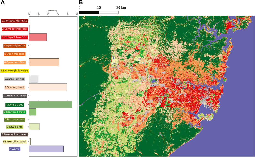
FIGURE 2. Local Climate Zone map of greater Sydney, Australia (B) obtained using local training areas and LCZ Generator tool (Demuzere et al., 2021) shown together with the histogram distribution of LCZ classes across the area (A).
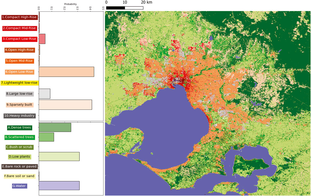
FIGURE 3. Same as Figure 2 for greater Melbourne, Australia.
2.2 Geoscape Derived Datasets
2.2.1 Land Cover Data
An independent high resolution dataset of two-dimensional land cover (Geoscape Surface Cover v1.6, 2020) was used to define surface cover fractions and enable comparison with the LCZ approach. The Geoscape surface data consists of 10 surface type categories at 2 m resolution, collected through remote sensing between 2017 and 2019, with coverage of all Australian towns and cities with populations greater than 200 persons. Coverage outside of urban areas is also available at 30 m resolution across the Australian continent (not used). Accuracy of land cover classification is greater than 90% (Geoscape Surface Cover v1.6, 2020). Using the 2 m urban data for two Australian cities, Sydney and Melbourne, we resample the ten Geoscape surface classes into six primary categories and two secondary categories (Table 3) at 100 m resolution. Cloud and shadow categories are not retained but are used to rescale other fractions so that primary and secondary categories each sum to 1 within grids.
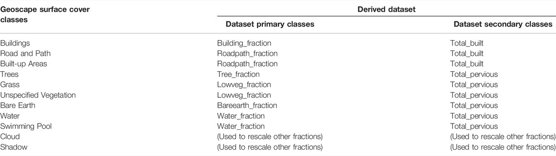
TABLE 3. Surface cover categories for the original Geoscape data and the derived dataset.
2.2.2 Morphology Data
Three-dimensional morphology data are derived from the datasets of buildings (Geoscape Buildings v2.0, 2020) and trees (Geoscape Trees v1.6, 2020). The buildings data consist of geolocated outlines of buildings within Australia with area greater than 9 m2 (approximately 15 million buildings), along with associated building metadata such as roof height. Trees data are raster-based with canopy height at 2 m resolution. Buildings and Trees datasets were collected through remote sensing (predominantly between 2017 and 2019) and processed through automated and manual processes using satellite-derived Digital Surface Model (DSM) or Digital Elevation Model (DEM) and aerial-derived stereo digitisation information. Vertical accuracy is approximately 0.1 m for aerial and 1 m for satellite derived building and tree heights. Horizontal accuracy is approximately 0.2 m for aerial and 2.5 m for satellite derived positioning (Geoscape Buildings v2.0, 2020; Geoscape Trees v1.6, 2020).
With these datasets we derive a range of gridded morphological statistics that are commonly used in urban modelling and observational studies (source code available in Supplementary Material). First, we calculate each building’s external wall area by multiplying building perimeter with building height (defined here as the average of building roof and eave heights), and each building’s frontal area is calculated by averaging the cross-sectional area of a building in two cardinal directions. These building-specific parameters are then used to calculate gridded statistics.
The gridded mean, maximum and standard deviations of building height (
For gridded values, the centroid of a building is used to assign the grid in which the building parameters will be placed. Trees are treated differently, as the underlying canopy height data are as rasterised canopy height at 2 m resolution. Tree-related parameters mean height (
Some urban models, such as TARGET (Broadbent et al., 2019) or UT&C (Meili et al., 2020), use inputs such as canyon aspect ratio (
where
In this dataset
To calculate momentum fluxes and wind profiles, some models require aerodynamic roughness lengths (
Using Macdonald et al. (1998), the zero-plane displacement height
where
Using Kanda et al. (2013), the zero-plane displacement height
where
Macdonald and Kanda derivations of
2.2.3 Processing and Resolution
We produce output at three resolutions (30, 100, and 300 m) to obtain gridded maps of city-descriptive parameters listed in Table 2. Figure 4 shows how different resolutions impact calculations of gridded sky view factor from the high-resolution building height data for a freely available sample of the Sydney data (https://geoscape.com.au/get-sample/). Figure 5 shows spatial maps of Sydney at 100 m resolution for a selection of the derived parameters. Our source code for producing outputs are included in Supplementary Material. We also make openly available a 300 m resolution derived dataset for the Greater Sydney region (Lipson et al., 2022), with outputs available in NETCDF and TIFF formats.
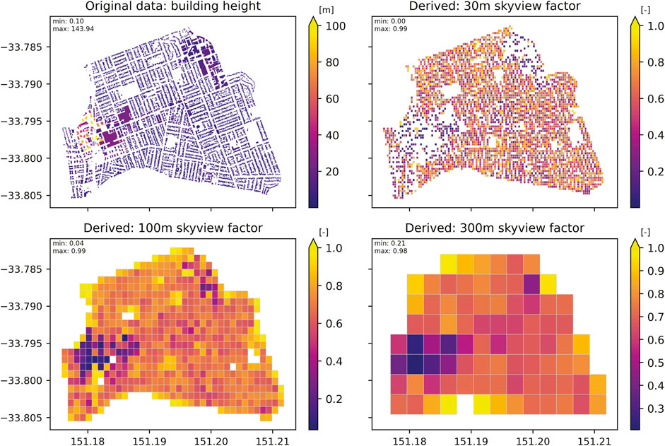
FIGURE 4. A sample of Geoscape data at original building level as well as processed data at 30 m, 100 m, and 300 m resolutions for sky view factor
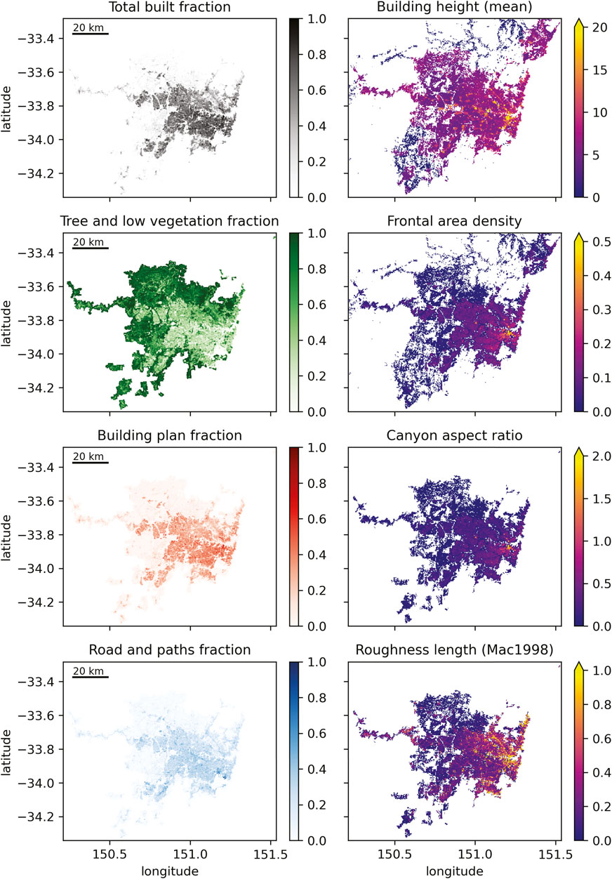
FIGURE 5. Select derived parameters for the Sydney region at 300 m resolution. Equivalent for Melbourne in Supplementary Material.
Surface cover fractions are calculated by summing all 2 m land cover categorical cells within each 30, 100 or 300 m grid, and dividing by the total cell instances within the larger grid. Gridded morphology characteristics are calculated by averaging (or finding the maximum and minimum) values for individual buildings where their footprint centroid falls within a grid.
When processing Geoscape data, the grid resolution has a critical impact on the calculated morphology parameters (Figure 4). While higher resolution may be desirable for some use cases (e.g., micro climate modelling), high resolution may not be appropriate for parameters intended to represent neighbourhood-scale characteristics. For example, canyon height-to-width ratio (
One alternative method is to divide each building that falls within multiple grids into smaller buildings with shared walls. This solution, however, increases the computational cost by more than 250 times in our small-scale tests, which meant it was not feasible to implement across a large geographic area such as Sydney. This solution also leads to overestimation of external wall area properties and associated parameters such as
The most appropriate output resolution will depend on the use case and available computational resources. Stewart and Oke (2012) define the intended scale of LCZs as spanning hundreds of metres to several kilometres in horizontal scale. For our comparison between Geoscape and LCZ outputs we used 100 m resolution to align with the native resolution of the LCZ generator output (Demuzere et al., 2021). Additional plots of parameter/resolution sensitivity (as in Figure 4) and for Melbourne outputs (as in Figure 5) are available in Supplementary Material (Supplementary Figures S2–S5) showing gridded building footprint fractions, pervious fractions, mean building heights, and canyon aspect ratios calculated from the high-resolution building footprint and building height data.
2.2.4 Comparison of LCZ With Derived Morphology Maps
Fine-grained data on urban form and fabric can inform numerical climate models which rely on categorical urban classifications. Through the WUDAPT project, several mesoscale climate models—including Weather Research Forecasting (WRF)—are now able to incorporate LCZ maps at 100–1,000 m resolutions (e.g., Brousse et al., 2016). Typically, the dominant LCZ type within a model grid is used to determine model parameters. More realistic inter-grid variability may be achieved by interpolating LCZ parameter values from higher-resolution maps to the model grid (Zonato et al., 2020). In either case, providing locally appropriate parameter values for each LCZ class has the potential to improve model performance compared with using generic LCZ characteristics.
To find locally appropriate LCZ characteristics, the coordinates of Geoscape-derived data are matched with LCZ maps at 100 m resolution. The Geoscape dataset is then grouped based on the corresponding grid’s LCZ categorization. Results are shown with a boxplot visualization, indicating mean and median values as well as data frequency distribution in each LCZ. The recommended parameter range and mean value for each LCZ class (Stewart and Oke, 2012) is also shown. This comparison focuses on six out of seven geometric and surface cover parameters defined for LCZs, covering pervious and impervious surface fraction, plan area density, sky view factor and height of roughness elements. Terrain roughness class is not included as it is not available through the Geoscape dataset.
3 Results
Figures 6–10 compare the recommended parameter ranges defined by Stewart and Oke (2012) for each LCZ class with local values obtained from the Geoscape surface cover, building and tree data for greater Sydney and Melbourne.
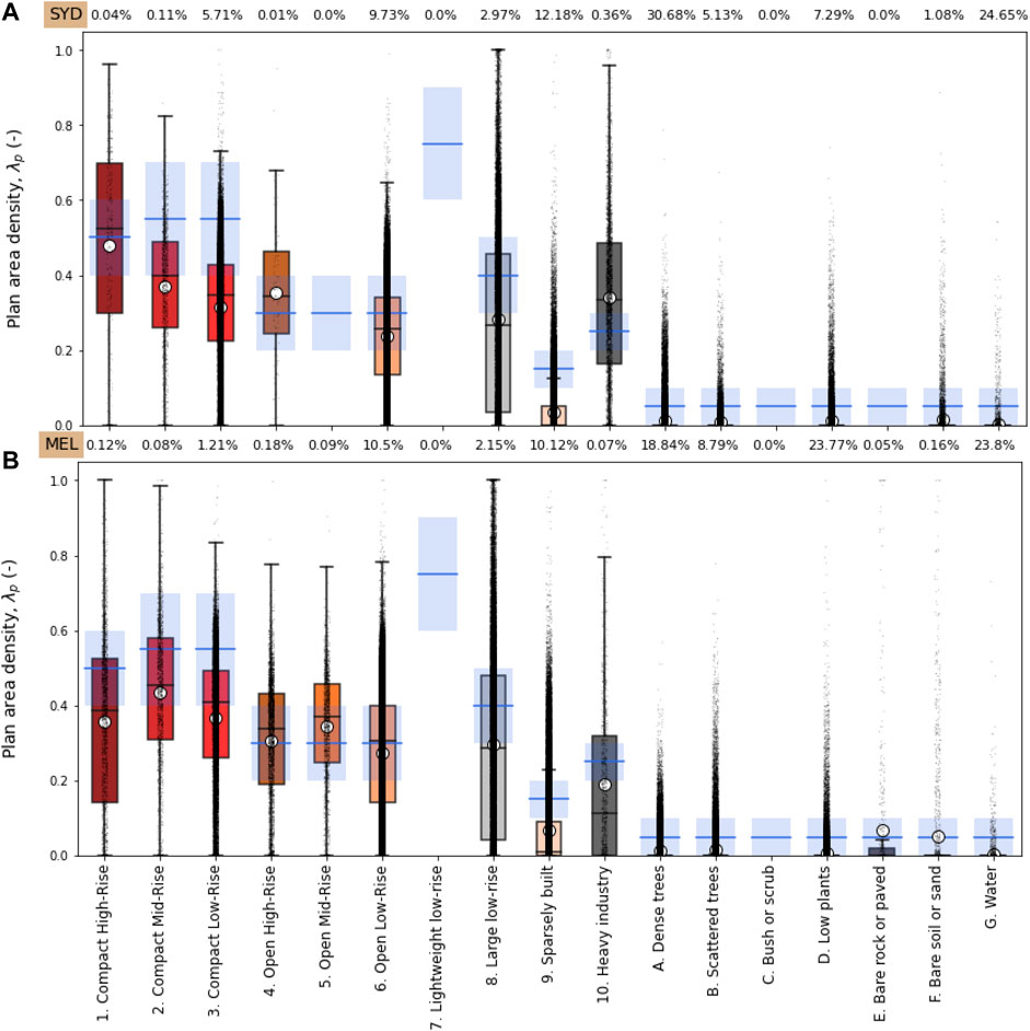
FIGURE 6. The range of building surface fraction or plan area density (
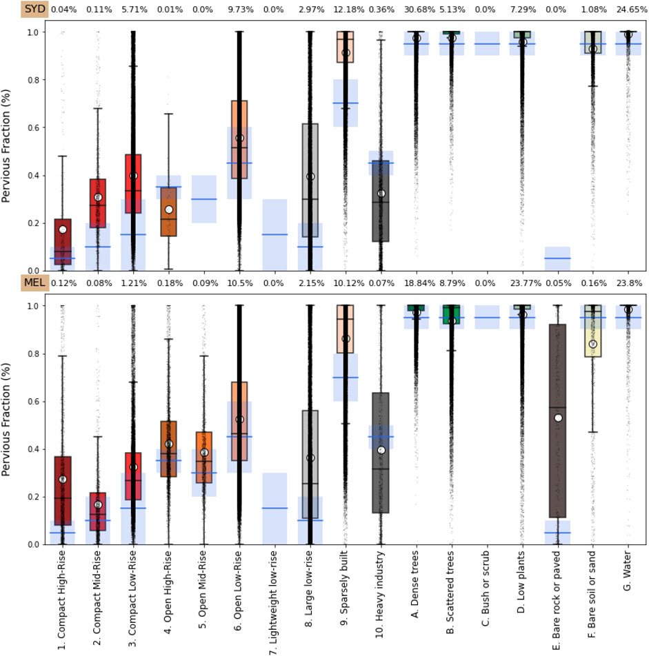
FIGURE 7. Same as Fig.6 for pervious fraction (including vegetation and water cover).
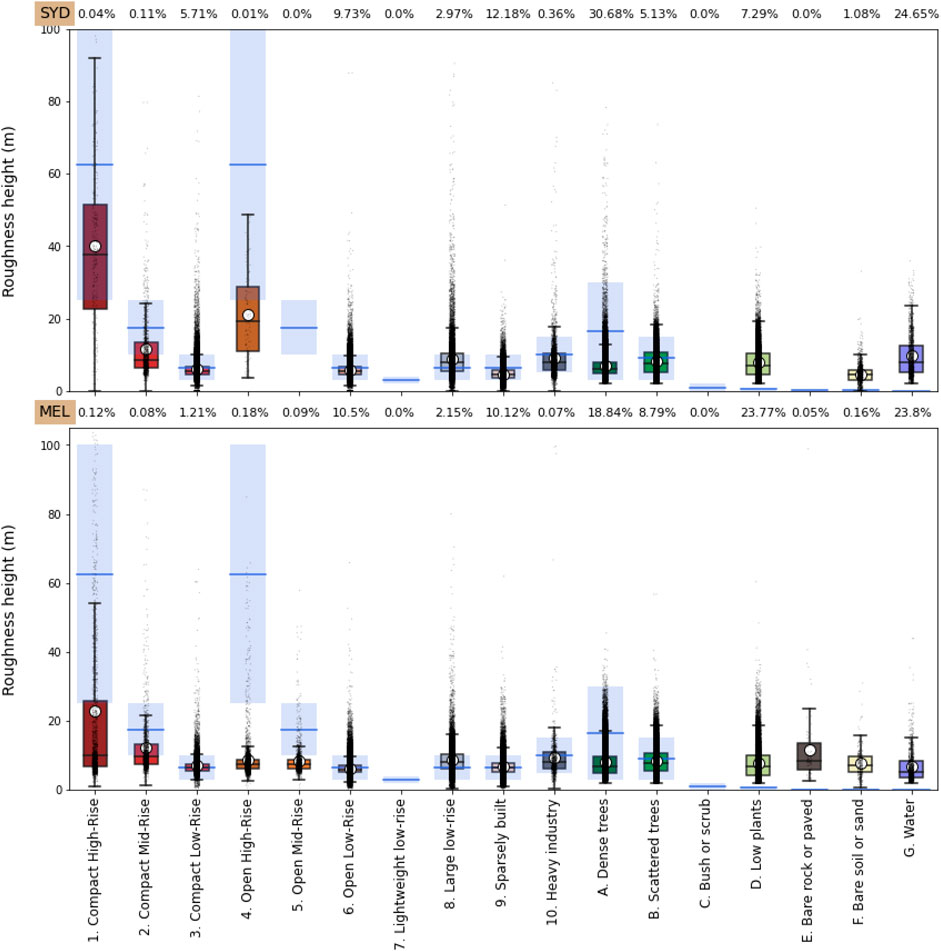
FIGURE 8. Same as Figure 6 for height of roughness element (geometric average of building heights (LCZs 1–10) and tree/plant heights (LCZs A–F) corresponding to Stewart and Oke (2012). Note- roughness height for LCZ 1 compact high-rise is given in Stewart and Oke (2012) as >25 m.
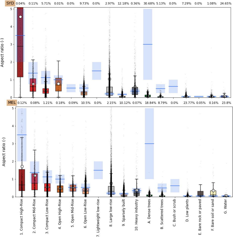
FIGURE 9. Same as Figure 6 for canopy aspect (heigh-to-width) ratio.
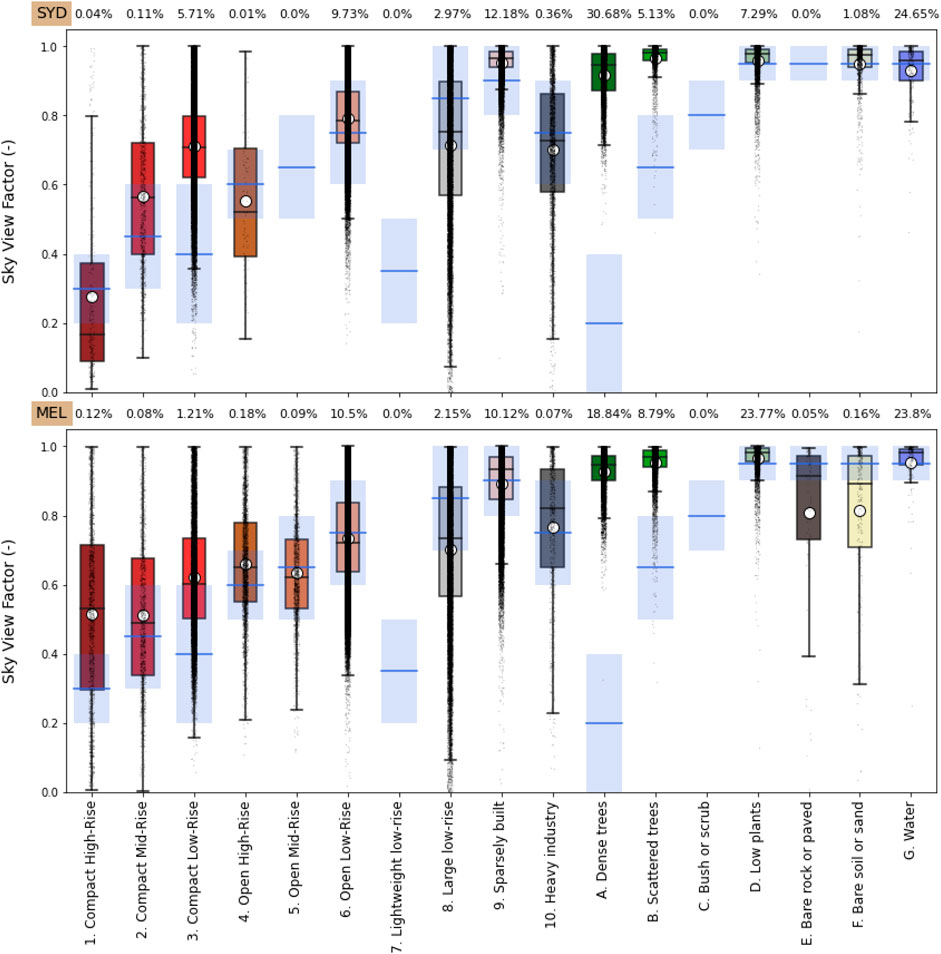
FIGURE 10. Same as Figure 6 for sky view factor.
For plan area density (Figure 6), the recommended LCZ range by Stewart and Oke (2012) shows reasonable agreement with the bottom-up data, although local values for both Sydney and Melbourne are generally lower. The difference is greatest in compact mid-rise (LCZ2), compact low-rise (LCZ3), large low-rise (LCZ8) and sparsely-built (LCZ9). The lower than recommended plan area density is seen consistently in both cities. This indicates that, although the WUDAPT instructions to derive LCZ classes were followed (including training data provided by local experts), differences with the original LCZ definitions can occur. The significant number of outliers in Figure 6 (and Figures 7–10) indicate the large variability of morphology characteristics within an LCZ class, as well as possible misclassification from the LCZ process.
Comparing the pervious fraction (Figure 7), the locally derived values are higher than recommended LCZ ranges in almost all built-up densities, except heavy industry. This difference is seen in both cities. Overall, this indicates that Australian cities have a higher percentage of vegetation and water even in compact neighbourhoods compared with LCZ-based definitions. Greater disparity occurs in categories for which there are few identified cells within the domain, for example LCZ1 (Compact high-rise) and LCZ4 (Open high-rise). For the natural land covers, good agreement is seen between both datasets.
Figure 8 compares the height of roughness elements in both datasets, as defined by Stewart and Oke (2012) as the geometric average of building heights in urban LCZ (LCZ 1-10) and tree/plant height for natural LCZs (LCZ A-F). The mean roughness height is significantly lower than the recommended range for the high-rise LCZ categories (LCZ 1 and LCZ3), particularly in Melbourne. This is likely because of different notions of what comprises a compact or open high-rise neighbourhood in Australian cities, and because compact and open high-rise neighbourhoods in Australian cities are less homogenous, i.e., high-rise buildings are surrounded by a range of different buildings with variable heights. This heterogeneity in the grids classified as “high-rise” consequently reduces the mean roughness height. The difference between the two maps is less pronounced in mid-rise LCZs, while LCZs with low building heights (such as compact/open/large low rise, sparsely built, and heavy industry) closely follow the recommended LCZ ranges. For natural land cover, when roughness height is calculated based on tree height (Stewart and Oke 2012), the bottom-up approach gives results within the recommended range for trees, but overestimates roughness element height in LCZs with low vegetation or no vegetation. This again could be caused by real urban heterogeneous surfaces including a scattering of higher roughness elements.
Two morphological parameters are also compared: Canopy aspect ratio (Figure 9) and sky view factor (Figure 10). These calculations are based on the assumption of a repeating, two-dimensional canyon geometry (Section 2.2) and depend on the calculated plan area and wall density (Masson et al., 2020) (
Although these results highlight some differences with recommended LCZ parameter values, the outputs provide valuable input data for urban climate models. The defined LCZ maps, when used to configure a model in Sydney or Melbourne, can now be informed with accurate local parameter values for each class. As such, we provide tables of urban LCZs (LCZ1-10; Table 4) and natural LCZs (LCZA-G; Table 5) for both Sydney and Melbourne for use in future modelling exercises. Mean values are calculated by comparing LCZ maps with 100 m morphology and surface cover data derived from Geoscape datasets. These provide a more accurate representation of local surface cover and morphology than the mid-point of the recommended LCZ ranges from Stewart and Oke (2012).
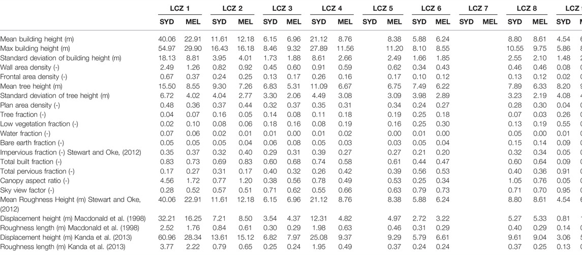
TABLE 4. City-descriptive parameters for Melbourne and Sydney for built-up local climate zones (LCZ 1-10). Mean values are calculated with gridded morphology and surface cover obtained from building-resolving 3D dataset (Geoscape) for each LCZ within each city’s map.
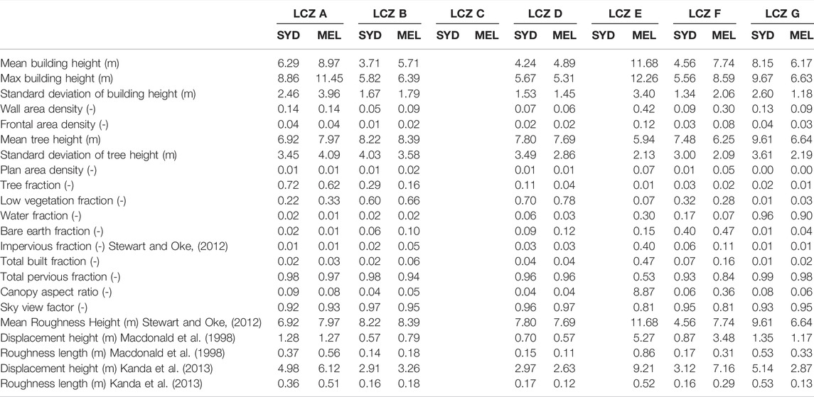
TABLE 5. City-descriptive parameters for Melbourne and Sydney for natural local climate zones (LCZ A-G). Mean values are calculated with gridded morphology and surface cover obtained from building-resolving 3D dataset (Geoscape) for each LCZ within each city’s map.
4 Discussion
Numerical urban analysis has been experiencing two critical transformations in the last decade. First, new datasets are being generated using novel methods describing urban form, fabric, and function at higher resolutions than previously achieved (Mills et al., 2021). Second, the growth of computing power—roughly doubling every 2 years (Leiserson et al., 2020)—has enabled more sophisticated models to resolve urban processes at higher resolutions. Nonetheless, many urban modelling studies have been unable to represent true intra-urban variabilities because they rely on class-based approaches to describe urban surface parameters.
In this paper, we presented a methodology to derive city-descriptive data for urban climate models using sub-metre resolution datasets which resolve individual urban elements. We have produced new gridded datasets which do not rely on classes. In addition, we have been able to complement established methods by updating default class-based parameters with those derived from local characteristics.
The code and examples for processing data layers are provided as Supplementary Material, enabling future city-descriptive maps to be developed for other regions using Geoscape data, as well as informing other studies with similar building-resolving datasets. The derived land cover and morphology dataset for the Greater Sydney region at 300 m resolution is made openly available (Lipson et al. 2022).
All building-resolving data contain errors which depend on the collection and processing methods. The base Geoscape data used here has a vertical accuracy of ±0.1 m for aerial and ±1 m for satellite derived building and tree heights (Geoscape Buildings v2.0, 2020; Geoscape Trees v1.6, 2020). The horizontal accuracy is ±0.2 m for aerial and ±2.5 m for satellite derived building positioning (although consistent translational errors minimise errors in the derived morphology characteristics). In comparison with top-down methods, the mid-range building height values for LCZs can differ with the Geoscape-derived values by dozens of metres (Figure 8), well outside the range of Geoscape errors. Top-down methods remain valuable where building-resolving data is unavailable.
The strength of the methodology described here is manifold. First, the building resolving data used is derived in a consistent manner at continental scales. Such large-scale and consistent datasets reduce uncertainties associated with class-based approaches which rely on ad-hoc human training and machine learning. Ad-hoc or inconsistent training data can lead to incorrect classification (Bechtel et al., 2017; Stewart, 2018), while machine learning inherently obscures the algorithm’s decision-making processes, making replication or adaptation difficult. Second, class-based approaches can omit some parameters required by numerical modelling systems. Our bottom-up method provides additional parameters for defining the form of urban areas and surrounds that are important for quantify the impact of mitigation strategies using modelling approaches (Krayenhoff et al., 2021). Lastly, the traditional class-based approach is limited by the fidelity of class system (i.e., the number of defined classes) while the bottom-up approach described here capture the unique characteristics of a city’s fabric and form by detailing variability at the grid scale. This is a methodological difference; instead of defining more subclasses at increasingly high fidelity and defining their recommended parameters, the properties of urban morphology can be captured from the building scale and applied at the desired resolution directly, enabling a more accurate characterization of real urban form in urban climate models.
The methods detailed here provide a useful approach for obtaining critical city-descriptive parameters for climate models, but several limitations persist. First, common geometric assumption used to calculate some morphology parameters (such as canopy height to width ratio and sky view factor) fall short in representing realistic urban configurations (as discussed in Section 2.2.3). Second, a method for resampling categorical class-based maps (the LCZ system) to different resolutions is not well-established in the literature, limiting the comparison of values at different resolutions. Thirdly, the data for large datasets may be remotely sensed and incorporated over time, and so should be updated regularly to account for rapid urbanization processes and changes in urban land cover and use. Furthermore, a key challenge in implementing this methodology relate to the availability of high-resolution datasets that resolve individual buildings and trees. Consistent and complete global high-resolution datasets are not yet publicly available. These challenges are likely to decrease as more data becomes available, though being significantly affected by different local data policy and resources (Mills et al., 2021). Finally, we still have limited available information on urban fabric and function, even at local scales. A description of the spatial distribution of materiality, for instance, is hard to achieve and hard to implement in models in a realistic way. These issues require more detailed attention in the future.
Data Availability Statement
The datasets presented in this study can be found in online repositories. The names of the repository/repositories and accession number(s) can be found in the article. The 300 m surface characteristics dataset is openly available for the Sydney region at: https://doi.org/10.5281/zenodo.6579061
Author Contributions
ML, NN, and MH conceived the study. BC and NN created the LCZ maps, with input from MH. ML wrote code to process Geoscape datasets and associated figures. NN wrote code to compare LCZ and Geoscape-derived outputs and associated figures. KN provided input for Melbourne data for comparison. NN, MH, and ML wrote the manuscript, with input from KN and BC.
Funding
This research was supported by the Australian Research Council (ARC) Centre of Excellence for Climate System Science (Grant CE110001028), the ARC Centre of Excellence for Climate Extremes (Grant CE170100023). KN is supported by NHMRC/UKRI grant (1194959).
Conflict of Interest
The authors declare that the research was conducted in the absence of any commercial or financial relationships that could be construed as a potential conflict of interest.
Publisher’s Note
All claims expressed in this article are solely those of the authors and do not necessarily represent those of their affiliated organizations, or those of the publisher, the editors and the reviewers. Any product that may be evaluated in this article, or claim that may be made by its manufacturer, is not guaranteed or endorsed by the publisher.
Acknowledgments
We gratefully acknowledge the Australian Urban Research Infrastructure Network (AURIN) and Geoscape Australia for providing the datasets necessary for this study, drawing on Geoscape Buildings, Surface Cover and Trees datasets, © Geoscape Australia, 2020: https://geoscape.com.au/legal/data-copyright-and-disclaimer/. With thanks to William Morrison, Sue Grimmond, Song Chen and Pratiman Patel for useful discussions on processing methods.
Supplementary Material
The Supplementary Material for this article can be found online at: https://www.frontiersin.org/articles/10.3389/fenvs.2022.866398/full#supplementary-material
Supplementary Figure S1 | Select derived parameters for the Melbourne region.
Supplementary Figure S2 | Building footprint fraction at 30, 100, 300 m resolutions for a sample region in Sydney.
Supplementary Figure S3 | Total pervious fraction at 30, 100, 300 m resolutions for a sample region in Sydney.
Supplementary Figure S4 | Mean building height at 30, 100, 300 m resolutions for a sample region in Sydney.
Supplementary Figure S5 | Canyon aspect ratio at 30, 100, 300 m resolutions for a sample region in Sydney.
References
Argüeso, D., Evans, J. P., Fita, L., and Bormann, K. J. (2014). Temperature Response to Future Urbanization and Climate Change. Clim. Dyn. 42, 2183–2199. doi:10.1007/s00382-013-1789-6
Bechtel, B., Alexander, P., Böhner, J., Ching, J., Conrad, O., Feddema, J., et al. (2015). Mapping Local Climate Zones for a Worldwide Database of the Form and Function of Cities. ISPRS Int. J. Geo-Inf. 4, 199–219. doi:10.3390/ijgi4010199
Bechtel, B., Alexander, P. J., Beck, C., Böhner, J., Brousse, O., Ching, J., et al. (2019). Generating WUDAPT Level 0 Data - Current Status of Production and Evaluation. Urban Clim. 27, 24–45. doi:10.1016/j.uclim.2018.10.001
Bechtel, B., Demuzere, M., Sismanidis, P., Fenner, D., Brousse, O., Beck, C., et al. (2017). Quality of Crowdsourced Data on Urban Morphology–The Human Influence Experiment (HUMINEX). Urban Sci. 1, 15. doi:10.3390/urbansci1020015
Biljecki, F., Chew, L. Z. X., Milojevic-Dupont, N., and Creutzig, F. (2021). Open Government Geospatial Data on Buildings for Planning Sustainable and Resilient Cities. ArXiv. Preprint 210704023 Cs. doi:10.48550/arXiv.2107.04023
Biljecki, F., Ledoux, H., and Stoter, J. (2016). An Improved LOD Specification for 3D Building Models. Comput. Environ. Urban Syst. 59, 25–37. doi:10.1016/j.compenvurbsys.2016.04.005
Broadbent, A. M., Coutts, A. M., Nice, K. A., Demuzere, M., Krayenhoff, E. S., Tapper, N. J., et al. (2019). The Air-Temperature Response to Green/blue-infrastructure Evaluation Tool (TARGET v1.0): an Efficient and User-Friendly Model of City Cooling. Geosci. Model Dev. 12, 785–803. doi:10.5194/gmd-12-785-2019
Brousse, O., Martilli, A., Foley, M., Mills, G., and Bechtel, B. (2016). WUDAPT, an Efficient Land Use Producing Data Tool for Mesoscale Models? Integration of Urban LCZ in WRF over Madrid. Urban Clim. 17, 116–134. doi:10.1016/j.uclim.2016.04.001
Bruse, M. (1999). The Influences of Local Environmental Design on Microclimate-Development of a Prognostic Numerical Model ENVI-Met for the Simulation of Wind, Temperature and Humidity Distribution in Urban Structures. Germany: University of Bochum.
Bureau of Meteorology (2021). Australia’s Official Weather Forecasts & Weather Radar - Bureau of Meteorology. Available at: http://www.bom.gov.au/(Accessed December 15, 2021).
Büttner, G. (2014). “CORINE Land Cover and Land Cover Change Products,” in Land Use and Land Cover Mapping in Europe: Practices & Trends Remote Sensing and Digital Image Processing. Editors I. Manakos, and M. Braun (Dordrecht: Springer Netherlands), 55–74. doi:10.1007/978-94-007-7969-3_5
Chen, G., Zhao, L., and Mochida, A. (2016). Urban Heat Island Simulations in Guangzhou, China, Using the Coupled WRF/UCM Model with a Land Use Map Extracted from Remote Sensing Data. Sustainability 8, 628. doi:10.3390/su8070628
Ching, J., Mills, G., Bechtel, B., See, L., Feddema, J., Wang, X., et al. (2018). WUDAPT: An Urban Weather, Climate, and Environmental Modeling Infrastructure for the Anthropocene. Bull. Am. Meteorol. Soc. 99, 1907–1924. doi:10.1175/BAMS-D-16-0236.1
Conroy, B. (2021). WUDAPT Level 0 Training Data for Melbourne (Australia, Commonwealth of), Submitted to the LCZ Generator. LCZ Gener. Available at: https://lcz-generator.rub.de/factsheets/d2aa6b283cdc6bf2dda372bfdcd5612d2219a690/d2aa6b283cdc6bf2dda372bfdcd5612d2219a690_factsheet.html (September 12, 2021).
Demuzere, M., Hankey, S., Mills, G., Zhang, W., Lu, T., and Bechtel, B. (2020). Combining Expert and Crowd-Sourced Training Data to Map Urban Form and Functions for the Continental US. Sci. Data 7, 264. doi:10.1038/s41597-020-00605-z
Demuzere, M., Kittner, J., and Bechtel, B. (2021). LCZ Generator: A Web Application to Create Local Climate Zone Maps. Front. Environ. Sci. 9, 112. doi:10.3389/fenvs.2021.637455
Esch, T., Brzoska, E., Dech, S., Leutner, B., Palacios-Lopez, D., Metz-Marconcini, A., et al. (2022). World Settlement Footprint 3D - A First Three-Dimensional Survey of the Global Building Stock. Remote Sens. Environ. 270, 112877. doi:10.1016/j.rse.2021.112877
Esch, T., Taubenböck, H., Roth, A., Heldens, W., Felbier, A., Thiel, M., et al. (2012). TanDEM-X Mission-New Perspectives for the Inventory and Monitoring of Global Settlement Patterns. J. Appl. Remote Sens. 6, 061702. doi:10.1117/1.JRS.6.061702
Fröhlich, D., and Matzarakis, A. (2020). Calculating Human Thermal Comfort and Thermal Stress in the PALM Model System 6.0. Geosci. Model Dev. 13, 3055–3065. doi:10.5194/gmd-13-3055-2020
Geoscape Surface Cover v1.6 (2020). Geoscape Surface Cover v1.6. Griffith, ACT, Australia: PSMA Australia.
Grimmond, C. S. B., and Oke, T. R. (1999). Aerodynamic Properties of Urban Areas Derived from Analysis of Surface Form. J. Appl. Meteor. 38, 1262–1292. doi:10.1175/1520-0450(1999)038<1262:apouad>2.0.co;2
Hirsch, A. L., Evans, J. P., Thomas, C., Conroy, B., Hart, M. A., Lipson, M., et al. (2021). Resolving the Influence of Local Flows on Urban Heat Amplification during Heatwaves. Environ. Res. Lett. 16, 064066. doi:10.1088/1748-9326/ac0377
Jackson, T. L., Feddema, J. J., Oleson, K. W., Bonan, G. B., and Bauer, J. T. (2010). Parameterization of Urban Characteristics for Global Climate Modeling. Ann. Assoc. Am. Geogr. 100, 848–865. doi:10.1080/00045608.2010.497328
Kanda, M., Inagaki, A., Miyamoto, T., Gryschka, M., and Raasch, S. (2013). A New Aerodynamic Parametrization for Real Urban Surfaces. Boundary-Layer Meteorol. 148, 357–377. doi:10.1007/s10546-013-9818-x
Katzfey, J., Schlünzen, H., Hoffmann, P., and Thatcher, M. (2020). How an Urban Parameterization Affects a High‐resolution Global Climate Simulation. Q.J.R. Meteorol. Soc. 146, 3808–3829. doi:10.1002/qj.3874
Krayenhoff, E. S., Broadbent, A. M., Zhao, L., Georgescu, M., Middel, A., Voogt, J. A., et al. (2021). Cooling Hot Cities: a Systematic and Critical Review of the Numerical Modelling Literature. Environ. Res. Lett. 16, 053007. doi:10.1088/1748-9326/abdcf1
Leiserson, C. E., Thompson, N. C., Emer, J. S., Kuszmaul, B. C., Lampson, B. W., Sanchez, D., et al. (2020). There’s Plenty of Room at the Top: What Will Drive Computer Performance after Moore’s Law? Science 368, eaam9744. doi:10.1126/science.aam9744
Li, D., Malyshev, S., and Shevliakova, E. (2016). Exploring Historical and Future Urban Climate in the Earth System Modeling Framework: 1. Model Development and Evaluation: Urban Climate in Earth System Models. J. Adv. Model. Earth Syst. 8, 917–935. doi:10.1002/2015MS000578
Lindberg, F., Grimmond, C. S. B., Gabey, A., Huang, B., Kent, C. W., Sun, T., et al. (2018). Urban Multi-Scale Environmental Predictor (UMEP): An Integrated Tool for City-Based Climate Services. Environ. Model. Softw. 99, 70–87. doi:10.1016/j.envsoft.2017.09.020
Lipson, M., Nazarian, N., Hart, M. A., Nice, K. A., and Conroy, B. (2022). Urban Form Data for Climate Modelling: Sydney at 300 M Resolution Derived from Building-Resolving and 2 M Land Cover Datasets. Sydney: Zenodo. doi:10.5281/ZENODO.6579061
Ma, S., Pitman, A., Yang, J., Carouge, C., Evans, J. P., Hart, M., et al. (2018). Evaluating the Effectiveness of Mitigation Options on Heat Stress for Sydney, Australia. J. Appl. Meteorol. Climatol. 57, 209–220. doi:10.1175/JAMC-D-17-0061.1
Macdonald, R. W., Griffiths, R. F., and Hall, D. J. (1998). An Improved Method for the Estimation of Surface Roughness of Obstacle Arrays. Atmos. Environ. 32, 1857–1864. doi:10.1016/S1352-2310(97)00403-2
Martilli, A., Krayenhoff, E. S., and Nazarian, N. (2020). Is the Urban Heat Island Intensity Relevant for Heat Mitigation Studies? Urban Clim. 31, 100541. doi:10.1016/j.uclim.2019.100541
Masson, V., Champeaux, J.-L., Chauvin, F., Meriguet, C., and Lacaze, R. (2003). A Global Database of Land Surface Parameters at 1-km Resolution in Meteorological and Climate Models. J. Clim. 16, 1261–1282. doi:10.1175/1520-0442-16.9.1261
Masson, V., Heldens, W., Bocher, E., Bonhomme, M., Bucher, B., Burmeister, C., et al. (2020). City-descriptive Input Data for Urban Climate Models: Model Requirements, Data Sources and Challenges. Urban Clim. 31, 100536. doi:10.1016/j.uclim.2019.100536
Meili, N., Manoli, G., Burlando, P., Bou-Zeid, E., Chow, W. T. L., Coutts, A. M., et al. (2020). An Urban Ecohydrological Model to Quantify the Effect of Vegetation on Urban Climate and Hydrology (UT&C v1.0). Geosci. Model Dev. 13, 335–362. doi:10.5194/gmd-13-335-2020
Middel, A., Nazarian, N., Bechtel, B., and Demuzere, M. (2022). Urban Climate Informatics: an Emerging Research Field. Front. Environ. Sci. Rev. 10, 867434. doi:10.3389/fenvs.2022.867434
Mills, G., Ching, J., and Bechtel, B. (2021). “Characterising Urban Morphology for Urban Climate Modelling,” in Urban Climate Science for Planning Healthy Cities Biometeorology. Editors C. Ren, and G. McGregor (Cham: Springer International Publishing), 339–354. doi:10.1007/978-3-030-87598-5_15
Mughal, M. O., Li, X. X., Yin, T., Martilli, A., Brousse, O., Dissegna, M. A., et al. (2019). High‐Resolution, Multilayer Modeling of Singapore's Urban Climate Incorporating Local Climate Zones. J. Geophys. Res. Atmos. 124, 7764–7785. doi:10.1029/2018JD029796
Nazarian, N. (2022). WUDAPT Level 0 Training Data for Sydney (Australia, Commonwealth of), Submitted to the LCZ Generator. LCZ Gener. Available at: https://lcz-generator.rub.de/factsheets/3530917846fefde7c17637092c9b98a2378053e0/3530917846fefde7c17637092c9b98a2378053e0_factsheet.html (January 27, 2022).
Nice, K. A., Coutts, A. M., and Tapper, N. J. (2018). Development of the VTUF-3D v1.0 Urban Micro-climate Model to Support Assessment of Urban Vegetation Influences on Human Thermal Comfort. Urban Clim. 24, 1052–1076. doi:10.1016/j.uclim.2017.12.008
Núñez-Peiró, M., Sánchez-Guevara Sánchez, C., and Neila González, F. J. (2021). Hourly Evolution of Intra-urban Temperature Variability across the Local Climate Zones. The Case of Madrid. Urban Clim. 39, 100921. doi:10.1016/j.uclim.2021.100921
Oleson, K. W., and Feddema, J. (2020). Parameterization and Surface Data Improvements and New Capabilities for the Community Land Model Urban (CLMU). J. Adv. Model. Earth Syst. 12, e2018MS00158. doi:10.1029/2018MS001586
Potgieter, J., Nazarian, N., Lipson, M. J., Hart, M. A., Ulpiani, G., Morrison, W., et al. (2021). Combining High-Resolution Land Use Data with Crowdsourced Air Temperature to Investigate Intra-urban Microclimate. Front. Environ. Sci. 9, 385. doi:10.3389/fenvs.2021.720323
PSMA Australia (2020). Geoscape | Location Data with Depth. Geoscape Aust. Available at: https://geoscape.com.au/(Accessed December 15, 2021).
Simón‐Moral, A., Dipankar, A., Roth, M., Sánchez, C., Velasco, E., and Huang, X. Y. (2020). Application of MORUSES Single‐layer Urban Canopy Model in a Tropical City: Results from Singapore. QJR Meteorol. Soc. 146, 576–597. doi:10.1002/qj.3694
Sirko, W., Kashubin, S., Ritter, M., Annkah, A., Bouchareb, Y. S. E., Dauphin, Y., et al. (2021). Continental-scale Building Detection from High Resolution Satellite Imagery. arXiv. Preprint. doi:10.48550/arXiv.2107.12283
Siu, L. W., and Hart, M. A. (2013). Quantifying Urban Heat Island Intensity in Hong Kong SAR, China. Environ. Monit. Assess. 185, 4383–4398. doi:10.1007/s10661-012-2876-6
Stewart, I. (2018). Developing a Field Guide to Identify Local Climate Zones in Cities. in Special Session on World Urban Database and Access Portal Tools (WUDAPT) I. New York: American Meteorological Society. Available at: https://ams.confex.com/ams/ICUC10/meetingapp.cgi/Paper/342085.
Stewart, I. D., and Oke, T. R. (2012). Local Climate Zones for Urban Temperature Studies. Bull. Am. Meteorol. Soc. 93, 1879–1900. doi:10.1175/bams-d-11-00019.1
Sun, Z., Du, W., Jiang, H., Weng, Q., Guo, H., Han, Y., et al. (2022). Global 10-m Impervious Surface Area Mapping: A Big Earth Data Based Extraction and Updating Approach. Int. J. Appl. Earth Observation Geoinformation 109, 102800. doi:10.1016/j.jag.2022.102800
Zhang, X., Liu, L., Wu, C., Chen, X., Gao, Y., Xie, S., et al. (2020). Development of a Global 30 m Impervious Surface Map Using Multisource and Multitemporal Remote Sensing Datasets with the Google Earth Engine Platform. Earth Syst. Sci. Data 12, 1625–1648. doi:10.5194/essd-12-1625-2020
Keywords: urban, climate, model, spatial, data, open, morphology
Citation: Lipson MJ, Nazarian N, Hart MA, Nice KA and Conroy B (2022) A Transformation in City-Descriptive Input Data for Urban Climate Models. Front. Environ. Sci. 10:866398. doi: 10.3389/fenvs.2022.866398
Received: 31 January 2022; Accepted: 06 June 2022;
Published: 06 July 2022.
Edited by:
Marco Casazza, University of Salerno, ItalyReviewed by:
Saskia Buchholz, German Weather Service, GermanyAndrea Zonato, University of Trento, Italy
Merja H. Tölle, University of Kassel, Germany
Jack Katzfey, CSIRO Oceans and Atmosphere, Australia
Copyright © 2022 Lipson, Nazarian, Hart, Nice and Conroy. This is an open-access article distributed under the terms of the Creative Commons Attribution License (CC BY). The use, distribution or reproduction in other forums is permitted, provided the original author(s) and the copyright owner(s) are credited and that the original publication in this journal is cited, in accordance with accepted academic practice. No use, distribution or reproduction is permitted which does not comply with these terms.
*Correspondence: Mathew J. Lipson, bS5saXBzb25AdW5zdy5lZHUuYXU=