Effects of Climate Change on Hydrological Indicators of Subsurface Drainage for a Representative French Drainage Site

The aim of this study is to evaluate from a hydrological perspective and in the context of climate change the future of subsurface drainage of the La Jaillière site (western France), which is representative of the pedology of the majority of French subsurface drainage. We used a uniquely large and comprehensive range of 17 hydrological indicators (HIs), describing the temporal dynamics of drainage season, soil saturation, drained water balance and flood events. The HI values are calculated from simulated discharges provided by a subsurface drainage model, the SIDRA-RU model, fed by 12 climate projections from 1975 to 2100 (CMIP5 Euro-Cordex project), with three climate change scenarios: Representative Concentration Pathways (RCP) 2.6, RCP4.5 and RCP8.5. We first verified that the HIs simulated using climate projections in the SIDRA-RU model over the historical period were not critically biased compared to the HIs obtained from the reference climatic reanalysis (SAFRAN). Second, we analysed and compared the HI evolution over different periods and under different scenarios. Our results showed that the number of significant changes in HI values increased under climate change by 2100, depending on the RCP: 2 HIs out of the 17 changed under RCP2.6; 6 HIs under RCP4.5; 10 HIs under RCP8.5. The intensity of drainage peak flows linked to flood events and the annual maximal discharge changed significantly under all RCPs. The temporality of the drainage season was substantially affected according to how pessimistic the RCP was. The worst changes were observed under RCP8.5, which exacerbated extreme events: The wet period was shorter while the dry period was longer by about 67%; the drought index increased by 100%; the summer drained water balance decreased by 9%. On the contrary, in winter, the duration of the wet period decreased while maintaining the same drained water balance, thus inducing stronger flood events leading to an earlier saturation of the drainage networks. The sustainability of the drainage system design at La Jaillière is therefore threatened, with the risk of fulfilling its function less effectively by 2100, exposing current crops to more important runoff and affecting water quality by increasing the leaching of agrochemical inputs.

Introduction

In its successive reports, the IPCC stated that the climate will be subject to several changes by 2100, including an increasing number of rapid and intense events (Garner et al., 2015), such as flash floods (Kundzewicz et al., 2014; Yin et al., 2016; Xu et al., 2019; Zhang et al., 2019), and a global increase in air temperature (IPCC, 2008, 2014) resulting in more frequent drought events (Prudhomme et al., 2014). Numerous studies have been carried out to assess the impact of climate change on the hydrological cycle, both at the catchment and regional levels, mostly on hydrologically unmodified systems and at large spatial scales (Khaliq et al., 2009; Arnell and Gosling, 2016; Carvalho-Santos et al., 2016; Lemaitre-Basset et al., 2021).

The future of subsurface drainage hydrology under climate change is also assessed but sometimes studies reports contrasting results. Sojka et al. (2020) and Pease et al. (2017) found that the annual drained water balance decreases in central western Poland, and in the north-eastern United States (United States), respectively. Some studies, however, show the opposite pattern in eastern Canada and Quebec (Dayyani et al., 2012; Mehan et al., 2019; Jiang et al., 2020; Golmohammadi et al., 2021), even among sites from the same geographical area. Furthermore, making broad conclusions about the future of subsurface drainage under climate change, e.g. using a meta-analysis procedure, is particularly challenging due to the lack of available studies on this topic. A case-by-case study is then one of the remaining ways to assess the future of subsurface drainage system in view of possible and appropriate improvements. Indeed, the sustainability of the drainage network design, i.e. its capacity of fulfilling its function in the current design, is questioned (Deelstra, 2015; Abd-Elaty et al., 2019; Sojka et al., 2020), since the depth and spacing between each drain may no longer be suitable for future conditions. Stable hydric conditions in drained plots are no longer guaranteed, as they are exposed to more frequent flood events under climate change (IPCC, 2014) or drought events that increase crop water demand to which farmers may respond with increasing irrigation (Grusson et al., 2021).

Assessing subsurface drainage future is a key point to mitigate or adapt to the impacts of climate change on the concerned lands, especially regarding crop yields. Currently used on plots that show infiltration issues such as hydromorphic soils (Jamagne, 1968; Thompson et al., 1997; Baize and Jabiol, 2011; Lange et al., 2011), subsurface drainage is a soil management technique that consists in introducing a network of perforated pipes into the ground to facilitate water infiltration and reduce surface runoff (Henine et al., 2014; Tuohy et al., 2018). In Europe, the proportion of drained agricultural lands varies across countries depending on pedological properties, climate conditions and agricultural policies. Higher proportions are observed in northern Europe with more than 50% in the United Kingdom, the Netherlands and Finland, while in southern countries the proportions are lower, such as Belgium (from 10 to 20%), France and Spain (below 10%) (ICID, 2021). In France, subsurface drainage plays an important role in the environment and in the dynamics and quality of water resources (Tournebize et al., 2012; Tournebize et al., 2017; Lebrun et al., 2019). To adapt subsurface drainage management sustainably, it is therefore essential to assess and understand its functioning under climate change.

Studies dealing with subsurface drainage differ in their view of the subsurface drainage and in their choice of hydrological indicators (HIs) with which to study the system. One limitation characterizing these studies comes from the low number of HIs commonly used to describe the subsurface drainage hydrology. Usually, HIs deal with the drained water balance (Dayyani et al., 2012; Mehan et al., 2019; Golmohammadi et al., 2021) and the daily discharge (Pease et al., 2017; Jiang et al., 2020). However, these characteristics do not offer a precise description of the future of subsurface drainage. On the contrary, indicators describing flood events, such as the flashiness index (Deelstra, 2015) that indicates the speed of change from one state to another, can be useful for describing drainage dynamics. Other HI classes helping farmers in the management of pollutants can also be particularly relevant, such as the beginning of the drainage season (Henine et al., 2022) or the duration of soil dryness or saturation. Introducing these new HI classes in drainage research can help gain knowledge about the future of subsurface drainage, providing useful information to the stakeholders concerned.

Running a hydrological model with climate change scenarios is a classic method for assessing the impact of climate change on hydrology (Arnell and Reynard, 1996; Prudhomme et al., 2010; Charlton and Arnell, 2014). A common approach is to use climate projections following different Representative Concentration Pathways (RCPs) induced by greenhouse gas emissions by 2100 (Moss et al., 2008; Kalantari, 2011; IPCC, 2014; Nam et al., 2015; Mukundan et al., 2020). Although useful, this method may induce biases in the calculation of the HIs. For instance, it is strongly recommended to use several climate projections (i.e. using different general circulation models, GCMs, Randall et al. (2001); Mechoso and Arakawa (2003)) per RCP to better account for uncertainties (Shrestha et al., 2018). Assessing and integrating them is therefore a necessary step that must be carefully addressed and is given specific attention in the present paper.

The aim of this study is thus to assess the future of subsurface drainage under climate change in one specific French drained plot in the La Jaillière site in western France, chosen for its representativeness of French subsurface drainage. To our knowledge, this is the first analysis of climate change effects on drainage in France. We use 30 Euro-Cordex future climate projections distributed over three RCPs: RCP2.6, RCP4.5 and RCP8.5. These climate projections feed the subsurface drainage model SIDRA-RU (Henine et al., 2022), a lumped and parsimonious model which has demonstrated good performance and temporal robustness in simulating subsurface drainage fluxes in France (Jeantet et al., 2021). The SIDRA-RU model provides subsurface drainage discharges, which then allow us to calculate 17 hydrological indicators specific to subsurface drainage, which constitute a uniquely large range of complementary indicators and give a comprehensive view of the subsurface drainage response. First, we assess the potential bias induced by the use of the climate projections in the SIDRA-RU model on these indicators over a historical period (1975–2004). Second, we analyse the evolution of the indicators from the historical period to a future period (2006–2099) in order to assess the potential impact of climate change on subsurface drainage in La Jaillière.

Materials and Methods

Study Site

The La Jaillière site (Figure 1) is an experimental station located in the Loire-Atlantique region in western France, managed by Cemagref and ITCF institutes between 1987 and 1999, and by Arvalis-“Institut du végétal” (Vegetal institute in France) from 1999 to the present. The soil of La Jaillière is hydromorphic and brown belonging to the Luvisol category (IUSS Working Group WRB, 2015; Dairon et al., 2017) with a loamy soil texture. This combination is found in approximately 80% of the total French drained areas (Lagacherie and Favrot, 1987) and is thus a good representative of French subsurface drained areas. La Jaillière is also a reference site as part of the EU agricultural experimental sites for the assessment of the dynamics of active pesticide substances in drained soils (FOCUS, 2012). Our study focuses on plot T4 (Figure 1) that covers 0.9 ha and is characterized by a mainly silty-sandy soil texture at the soil horizon (20–25% clayey, 40–45% silty, 30–40% sandy) and silty-clayey texture in the lower horizon (40–50% clayey, 35% silty, 15–25% sandy).

FIGURE 1

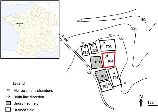
FIGURE 1. Experimental study site of La Jaillière. Adapted from Henine et al. (2022).

The climate in the study site is oceanic with an annual cumulative rainfall and a mean potential evapotranspiration, respectively, of 709 and 738 mm, and with a mean annual temperature of approximately 11°C. A subsurface drainage system composed of perforated polyvinyl chloride (PVC) pipes drains the plot, with an inter-drain spacing of 10 m at an average depth of 0.9 m. The drainage network was settled in the 80s during campaigns managed by INRAE (formerly CEMAGREF) to evaluate drainage modalities according to pedological and climatic conditions. The water-holding capacity was estimated to be 104 mm (Henine et al., 2022). The crop system is a two-year rotation of winter wheat and maize. winter wheat is cultivated from the second half of October to the second half of the next July, while maize is cultivated from late April/early May to September. Cover crops are used once every two years in the period included from the harvest of winter wheat to the sowing of maize. The surface runoff is deemed negligible on this site (Kuzmanovski et al., 2015; Henine et al., 2022) and thus it was not studied here.

Input Data

The meteorological data used as a reference for the historical period were provided by the SAFRAN database (Vidal et al., 2010), supplying a meteorological reanalysis of precipitation (P) and potential evapotranspiration (PE, based on the FAO-56 Penman–Monteith PE formulation (Córdova et al., 2015)) over France. Data are available from 1959 to 2019 at a daily time step and on a regular grid of 8 × 8 km.

In this study, climate projection data were provided by six GCMs coupled with nine regional circulation models (RCMs) in order to spatially disaggregate data from GCMs. Due to the computation time limitations in generating the climate projections (CPs), not all GCM–RCM couples are available for every RCP (Table 1, Lemaitre-Basset et al., 2022). In our study, we considered 12 CPs (Soubeyroux et al., 2021) from the Euro-Cordex project (Jacob et al., 2014) selected by Météo-France to ensure the representativeness of future conditions in France. Post-treatment through the ADAMONT method (Verfaillie et al., 2017) was carried out on the CPs, first to correct bias versus SAFRAN data using the quantile–quantile mapping method (Maurer et al., 2010; Navarro-Racines et al., 2020; Potter et al., 2020), and second to downscale the CPs to the same spatial resolution as SAFRAN. These CPs provide simulations following three RCPs: the very stringent pathway RCP2.6 (van Vuuren et al., 2007), the intermediate pathway RCP4.5 (Thomson et al., 2011) and the worst-case pathway RCP8.5 (Riahi et al., 2011). Projections are available at a daily time step from 1975 to 2100 and are split into two parts:

- “Historical” from 1975 to 2004: All climate models are forced by the observed greenhouse gases concentrations. According to the hydrological year concept, we considered data from August 1, 1975 to July 31, 2004;

- “Projected” from 2006 to 2100: The projections are led by the RCPs, defining the evolution of greenhouse gas concentrations. As the year 2005 is the transitional year between the two periods, we excluded it from the analyses. Thus, we considered data from August 1, 2006 to July 31, 2099.

TABLE 1

TABLE 1. Availability of climate projections. The numbers (2.6, 4.5 and 8.5) refer to the RCPs used by the GCM (rows)/RCM (columns) pairs. “-” indicates the absence of data. Adapted from Lemaitre-Basset et al. (2022).

The SIDRA-RU Model

The hydrological model used in this study was the SIDRA-RU model (Henine et al., 2022), a four-parameter lumped and semi-conceptual model, designed to simulate subsurface drainage discharges from artificially drained plots. The model uses the principle of rainfall–discharge conversion being fed by daily precipitation P(t) (without distinguishing liquid and solid parts) and PE(t) to predict drainage discharge Q(t) at the drainage network outlet. First, an evapotranspiration module converts PET(t) into an approximate value of actual evapotranspiration, called corrected evapotranspiration CET(t), from the available water level S(t) in a conceptual storage to satisfy the evapotranspiration (see Eq. 1):

$CET\left(t\right)=PET\left(t\right)\ast e^{-\frac{S_{RFU}-S\left(t\right)}{S\left(t\right)}}(1)$

With $S_{RFU}$ a threshold assigning the minimal water level to fully satisfy PET(t). Let us note that current crop is not used to simulate CET, only depending on the water availability of the storage. Second, the net infiltration $P_{net}\left(t\right)$ is calculated by subtracting CET(t) from P(t) in order to simulate the water table recharge term R(t) (mm) using the RU module (“Réserve Utile” in French designated the water holding capacity of a soil). R(t) is simulated from the meteorological input and the available water level S(t) in the reservoir (see Eq. 2) distinguishing three situations:

$\{\begin{array}{l}if S\left(t\right)<S_{inter}: S\left(t\right)= S\left(t-1\right)+ P_{net}\left(t\right)| R\left(t\right)=0;\\ if S\left(t\right)\in \left[S_{inter};S_{max}\right[:S\left(t\right)= \left(1- \alpha \right) P_{net}\left(t\right)+S\left(t-1\right) | R\left(t\right)= \alpha \ast P_{net}\left(t\right);\\ if S\left(t\right)\ge S_{max}: S\left(t\right)= S_{max}| R\left(t\right)= P_{net}\left(t\right).\end{array}(2)$

With:

• $\alpha$ (-), proportion of $P_{net}\left(t\right)$ experimentally set at $1/3$ (Henine et al., 2022);

• $S_{inter}$ (mm), intermediate threshold of the soil reservoir defining the water quantity needed to generate flow in the reservoir before saturation of the storage ($S_{RFU}$ = 0.4* $S_{inter}$, Jeantet et al. (2021));

• $S_{max}$ (mm), parameter representing the maximal capacity of the soil reservoir from which the net infiltration is fully converted into R(t).

Let us note that $S_{inter}$ and $S_{max}$ are the two main parameters of the RU module, used to simulate some hydrological indicators (see Hydrological Indicators of Subsurface Drainage Section). Third, the physically-based SIDRA module (“SImulation du DRAinage” for drainage simulation in French) converts R(t) into Q(t) (see Eqs 3, 4), following the Boussinesq equation (Boussinesq, 1904):

$\frac{dh\left(t\right)}{dt}=\frac{R\left(t\right)-\mathrm{K}\frac{\mathrm{h}{\left(t\right)}^2}{{\mathrm{L}}^2} }{A_2\mu } ; h\left(t+1\right)=h\left(t\right)+ \frac{dh\left(t\right)}{dt}(3)$

$\mathrm{Q}\left(t\right)=\mathrm{AK}\frac{\mathrm{h}{\left(t\right)}^2}{{\mathrm{L}}^2}+\left(1-\mathrm{A}\right)\mathrm{R}\left(\mathrm{t}\right)(4)$

With:

• L: space between drain and inter-drain (m);

• A₂: second water table shape factor (Lesaffre, 1989), $A_2\approx 0.89$ (-);

• A: third water table shape factor (Lesaffre, 1989), $A=0.869$ (-). Here, we assume that the shape of the water table between the drain and the mid-drain is an ellipse. Therefore, A is obtained by integrating ¼ of this reference ellipse.

The SIDRA module is mainly controlled by two parameters: the horizontal hydraulic conductivity K (m.d⁻¹), and drainage porosity µ (-). The four calibrated parameters are K, µ, $S_{inter}$ and $S_{max}$. In this study, their values were extracted from the analysis of Jeantet et al. (2021). Unlike most current subsurface drainage models, the SIDRA-RU model use strong assumptions, such neglecting current crop to simulate CET. This assumption is based on the fact that, despite being managed by the two-year crop rotation winter wheat/maize and the absence/presence of cover crops, the water balance of the studied site is not affected by current crop (Henine et al., 2022). A more detailed description of the SIDRA-RU model is provided by Henine et al. (2022) and Jeantet et al. (2021).

Hydrological Indicators of Subsurface Drainage

To describe the future reaction of subsurface drainage systems as precisely as possible so as to help farmers and decision-makers, 17 HIs gathered into six classes were defined (see Table 2). The drained water balance and the water content in the storage categories are mainly used to evaluate the arable nature of a soil. The categories of annual flood events and the sustainability of the current networks are analysed to assess whether the drainage network is still able to reduce flooding or whether it requires resizing. Finally, the temporality of the drainage season and the temporal flow dynamic categories are useful for assessing the effects of hydrological changes on water quality due to pollutant leaching. These classes and indicators are further detailed below:

1) Temporality of the drainage season. Considering a hydrological year defined from August 1 to next July 31, we considered two HIs: the beginning of the drainage season and its length. The beginning of the drainage season is set to day d using the cumulative discharge at d Cum_Q(d) since the last August 1 (see Eq. 5):

$\left\{\begin{array}{l}on the day d:\mathrm{Cu}{\mathrm{m}}_{\mathrm{Q}}\left(\text{d}\right)\ge Cu{m}_{Drainage}\\ \left[d+1:d+5\right] :\mathrm{Cu}{\mathrm{m}}_{\mathrm{Q}}\left(\text{d}\right)\ge Cu{m}_{Drainage} +Cu{m}_{reliable}\end{array}\right\}(5)$

$Cu{m}_{Drainage}$ and $Cu{m}_{reliable}$ correspond to thresholds of cumulative discharges from the previous August 1, considered as minimum water quantities required to assess that the drainage season started at day d (Henine et al., 2022). They were experimentally set to 1.4 and 2.7 mm, respectively. The duration of the drainage season is defined as the number of days between the start and the end of the drainage season. The end of the drainage season is set on the first day d when the difference between the annual drained water balance on July 31, i.e. the end of the hydrological year, and Cum_Q(d) is lower than $Cu{m}_{Drainage}$;

2) Water content in the soil profile: the number of days the storage is saturated ($\text{S}\left(\text{t}\right)=S_{max}$) and the number of days the storage is close to being empty ($\text{S}\left(\text{t}\right)\le 25\text{ mm}$). Below 25 mm, the remaining stock is assimilated to non-available water to crops or PE demand. These two HIs are, respectively, defined as the wet index and the drought index;

3) Drained water balance: annual drained water balance (ADWB) and summer drained water balance (SDWB), for each hydrological year. The latter is set from April to September, i.e. until the end of the winter runoff to the end of the period when the soil storage is empty in most cases;

4) Temporal flow dynamics: the annual flow hydrograph is split into four phases per hydrological year (Humbert et al., 2015; Strohmenger et al., 2020): dry period, recharge period, wet period and recession period. The duration of each phase was analysed;

5) Annual flood events: a discharge $Q_d$ on day d is considered as a flood event following Eq. 6:

$\left\{\begin{array}{l}on the day d :Q_d\ge T_{flood}\\ on the day d+1 :Q_{d+1}\ge Q_d+T_{flood}\end{array}\right\}(6)$

TABLE 2

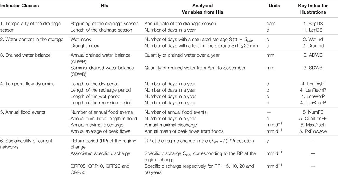
TABLE 2. Hydrological indicators (HIs) and corresponding variables analysed.

The threshold $T_{flood}$ is set to 1 mm d⁻¹ (Nedelec, 2005). A flood ends on day d following Eq. 7:

$\left\{\begin{array}{l}{Q}_d< T_{flood}\\ Q_d<0.8\ast Q_{flood\_max}\end{array}\right\}(7)$

with $Q_{flood\_max}$ the maximal discharge of the flood event (peak flow). The number of annual flood events, the annual cumulative duration in flood events, the annual maximal discharge and the annual mean of peak flows were considered;

6) Sustainability of the current networks: a regression analysis is carried out on the evolution of a specific discharge $Q_{spe}$ according to the associated return period (RP). The regime from the relation $Q_{spe}=f\left(RP\right)$ is characterized by two different linear regimes split by a breaking point close to 2 years, due to design criteria in order to intercept a rainfall of 15 mm d⁻¹ (Augeard et al., 2008; Henine et al., 2012). Above this value, the pipe is pressurized (Henine et al., 2010) and the specific discharge may be strongly reduced (Nedelec, 2005; Henine et al., 2012), according to the size of the networks and depending on the intensity of the event. If the RP of the breaking point decreases, the size of the networks might be considered as no longer suitable to fulfil efficiently their flood protection function. In this study, Hazen’s relation and the Gumbel distribution function (Gumbel, 1954) were used to establish the piecewise function of the regime and determine the breakpoint (see Eqs 8, 9) so as to assess its evolution under climate change:

$Q_{spe}=\{\begin{array}{l}{a}_1\ast u+ b_0 if u \le u_{RC};\\ a_2\ast u+a_1\ast u_{RC}+b_{0}if u >u_{RC};\end{array}(8)$

$u=ln\left[-ln\left(1-\frac{1}{RP}\right)\right](9)$

with:

➢ $u$: the change of variable in the Gumbel relation;

➢ $u_{RC}$: the change of variable corresponding to $R{P}_{RC}$, the RP at the regime change;

➢ $a_1$, $a_2$ and $b_0$: parameters from the non-linear regression.

The evolution of $Q_{spe}$ at RP = 5, 10, 20 and 50 years (QRP05, QRP10, QRP20 and QRP50) was also assessed.

Modelling Strategy

The modelling strategy is divided into three parts (Figure 2). First, we established reference hydrological indicators in the historical period (HI_REF) from 1975 to 2004 by simulating historical discharge using the SIDRA-RU model fed with the SAFRAN meteorological data. Second, the SIDRA-RU was fed with each historical CP to calculate all historical hydrological indicators (HI_{CP_HIST}) for the same historical period. Third, the SIDRA-RU was fed with the CPs in the future projected period, from 2006 to 2099. The future discharge series obtained were split into three continuous sub-periods, each one of approximately 30 years (Table 3) to represent the dispersion of climatic patterns (Soubeyroux et al., 2021). Then, we calculated future hydrological indicators (HI_{CP_FUTURE}) in the whole future period for HI classes 1–5 and in each future sub-period for HI class 6. Two sequences of analysis were performed: 1) the HI_REF and the HI_{CP_HIST} were compared to assess the bias induced by the use of climate projections in the SIDRA-RU model on the HIs; 2) the HI_{CP_FUTURE} were compared to the HI_{CP_HIST} to assess the impact of climate change on subsurface drainage hydrology.

FIGURE 2

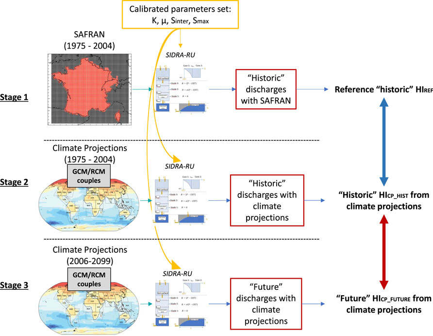
FIGURE 2. Stages of the modelling strategy. Adapted from Bourgin et al. (2010); IPCC, (2014); Jeantet et al. (2021).

TABLE 3

TABLE 3. Temporal split of the climate projections.

Evaluation of Bias From Projections in the SIDRA-RU Model Over the Historical Period

To assess the potential bias induced by the use of CPs in the SIDRA-RU model, the distribution functions of the HI_{CP_HIST} were compared with those from the HI_REF. We calculated the distribution functions from the HI values extracted on an annual basis and we then ranked them in ascending order. For each HI from classes 1 to 5 (Table 2), comparisons were made between the HI_{CP_HIST} from 12 different CPs (Table 1), i.e. from 12 series of HI_{CP_HIST} obtained for 30 hydrological years from 1975 to 2004. To avoid the comparison of each of these 12 series while preserving two samples of equivalent sizes, we averaged the 12 distribution functions of the HI_{CP_HIST} and compared the mean of the distribution function obtained to the corresponding HI_REF. The mean was calculated with a confidence interval at 95%, following a normal distribution (see Eq. 10, Saporta, (2006)):

$\left[\mu -t_{0.025,n-1}\ast \frac{ \sigma }{\sqrt{n}} ; \mu +t_{0.025,n-1}\ast \frac{ \sigma }{\sqrt{n}}\right](10)$

with:

➢ µ: the mean quantile from the distribution function from the CPs, per HI;

➢ $\sigma$: the associated standard deviation;

➢ $n$: the size of the sample, corresponding to the number of CPs tested (here, $n=12$);

➢ $t_{0.025}$: a coefficient used to establish a theoretical confidence interval at 95% according to $n$ (Barrett et al., 2015), assuming a normal distribution.

In practice, an initial graphic evaluation of quantile–quantile plots (Saporta, 2006) made it possible to compare the mean of the distribution functions of HI_{CP_HIST} with the distribution function of HI_REF. Second, we statistically tested the similarity between the HI_{CP_HIST} and the HI_REF by two non-parametric similarity tests: the Mann–Whitney–Wilcoxon test (Mann and Whitney, 1947; Hollander and Wolfe, 1973) and the Kolmogorov–Smirnov test (Birnbaum and Tingey, 1951; Conover, 1971). Third, two correlation tests were performed to assess the correlation between these two distribution functions: the Pearson test (Pearson and Galton, 1895) and the Spearman test (Spearman, 1904). The R package “stats” (R Core Team, 2021) was used for all these tests. The threshold for statistical significance was set at $p\le 0.05$.

For HI class 6 (see Table 2), the analyses consisted in a graphic comparison of specific discharges $Q_{spe}$ associated with RPs in the historical period (Table 1), namely between $Q_{spe}$ from the historical reference and those from CPs. Here, $Q_{spe}$ was associated with the annual maximal discharge $Q_{max}$, defined in HI class 5 (Table 2). $Q_{max}$ values from CPs were extracted from the mean of the distribution functions of $Q_{max}$ from the 12 CPs, calculated with a confidence interval at 95%. Then, piecewise functions (see Eq. 8) from both situations were fitted by a non-linear regression using smoothed $Q_{max}$ series and the R package “stats” to extract the parameters $a_1$, $a_2$ and $b_0$. Finally, RP values for the regime change were compared, along with the corresponding $Q_{max}$. Moreover, the QRP05, QRP10, QRP20 and QRP50 values from the historical reference were compared with those from CPs.

Evolution of the Hydrological Indicators in the Projected Period

For HI classes 1–5 (Table 2) and for each of the three RCPs, we calculated a 5-years rolling mean for the period 1975–2099 of each HI_{CP_HIST} and the associated HI_{CP_FUTURE} to assess the temporal trend of HIs in the future, with a confidence interval at 95%. Because of the CP data availability from 1975 to 2099, the rolling period was not centred on the first two years, i.e. 1975 and 1976, or the last two years, i.e. 2098 and 2099. As mentioned in Input data Section, the year 2005 was excluded from the analyses because it marks the transition from the projected past to the projected future. Therefore, the rolling period was not centred on 2003, 2004, 2006 and 2007 either. The significance of the trend of each HI_{CP_FUTURE} was assessed by performing a Mann–Kendall test (Mann, 1945; Hipel and McLeod, 1994) on both means and lower and upper limits of the confidence interval (R package “Kendall”, McLeod, (2011)). The threshold for statistical significance was set at $p\le 0.05$. In those cases, the trends were calculated as a percentage change from the HI_{CP_HIST} from the historical period 1975–2004 and the corresponding HI_{CP_FUTURE} from the future period PP3 (Table 3). The trends of HI_{CP_HIST} were calculated using the 12 CPs whereas the trends of HI_{CP_FUTURE} were calculated using the available CPs according to the corresponding RCP (Table 1).

For HI class 6, the analyses consisted in a graphic comparison between specific discharges $Q_{spe}$ associated with RPs from the historical period and those from the three future sub-periods (Table 1), all calculated from CPs. Similarly to the bias analysis for the historical period (Evaluation of Bias From Projections in the SIDRA-RU Model Over the Historical Period Section), the $Q_{spe}$ values from each future sub-period under each RCP (Table 3) were assimilated to the mean of the distribution functions of $Q_{max}$ from the available corresponding CPs (Table 1), supported by a confidence interval at 95%. Then, piecewise functions (see Eq. 8) were fitted by non-linear regression from the smoothed $Q_{max}$ of each case using the R package “stats”, and RP values for the regime change were compared, along with the corresponding $Q_{max}$. The deviations between the historical and future RPs at the regime changes RP_RC were calculated only if they were significant, i.e. if the confidence intervals from scatter plots were not superimposed close to the regime change, the same as for the corresponding discharges Q_RC. Moreover, the QRP05, QRP10, QRP20 and QRP50 values from the three future sub-periods were extracted from the previously fitted piecewise functions (see Eq. 8) and were compared with the values from the historical period.

Results

Evaluation of Potential Biases in HI Values From Climate Projections Over the Historical Reference

For the large majority of HIs, quantiles of HI_{CP_HIST} distributions were close to those of HI_REF following the 1:1 line, i.e. the line corresponding to the equation y = x (Figure 3 for HI classes 1–3 and Supplementary Appendix Figure SA1, for HI classes 4 and 5). Only a few extreme values (1–3 out of 30) from HI_{CP_HIST} showed stronger deviations compared to those from HI_REF in particular for the wet index (2.WetInd in Figure 3), the annual drained water balance (3.ADWB in Figure 3), showing the strongest deviations although rarely exceeding 10%, and the length of the wet period (4.LenWetP on Supplementary Appendix Figure SA1) that were deemed negligible.

FIGURE 3

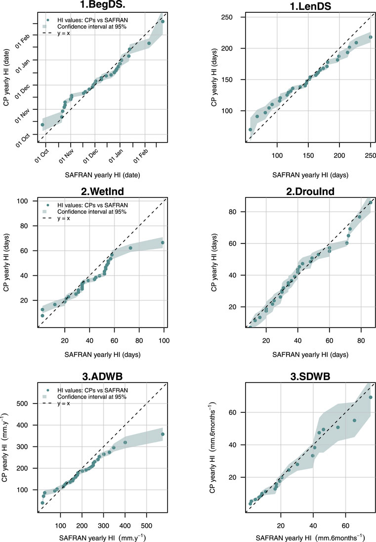
FIGURE 3. Distribution functions of HIs from CPs compared to those from SAFRAN in the historical period (1975–2004) for three classes of HIs: “Temporality of the drainage season”, “Water content in the storage” and “Drained water balance”. The distribution functions of HI_{CP_HIST} from CPs were calculated as the mean of distribution functions of HI_{CP_HIST} from the 12 CPs studied (Table 1). The abbreviated names of each HI referred to in the graphics are available in Table 2.

Results from the Mann–Whitney test and the Kolmogorov–Smirnov test showed no significant difference between the distribution functions of HI_{CP_HIST} and the distribution functions of HI_REF from classes 1 to 5, with all p values being higher than 0.05 (Table 4). In addition, the results from Spearman and Pearson correlation tests showed that for HI classes 1–5 the HI_REF and HI_{CP_HIST} trends were significantly correlated (p values ≤0.05), with correlation coefficients currently over 0.95. Overall, these results (graphical exploration and statistical testing) supported the hypothesis that for all the HIs from classes 1 to 5, the HI_{CP_HIST} and HI_REF distributions did not substantially differ, which allowed us to consider that no critical bias was exposed in the use of SIDRA-RU.

TABLE 4

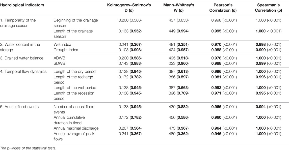
TABLE 4. Results of the significant tests and the correlation tests comparing the HI_{CP_HIST} and HI_REF distribution functions in the historical period (1975–2004).

The discrepancies between $Q_{max}$ associated with the RPs from the historical reference and those obtained from the CPs in the historical period were relatively small (≤2 mm d⁻¹) and deemed negligible (Figure 4). Let us note that $Q_{max}$ from the CPs appeared slightly underestimated compared to those from the historical reference, except for RPs shorter than 1.3 years. The two fitted piecewise functions, on $Q_{max}$ from the CPs and on $Q_{max}$ from the historical reference, were well fitted with respective small residual sum-of-squares of 0.79 and 1.98. The corresponding lines in Figure 4 show the regime change from CPs was 2 months late compared to the change from the historical reference, for an associated $Q_{max}$, respectively, equal to 12.3 mm d⁻¹ and 12.8 mm d⁻¹. The coordinates from both breaking points appeared close.

FIGURE 4

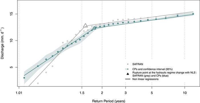
FIGURE 4. Comparison of the specific discharges $Q_{spe}$ (here the annual maximal discharge) associated with return periods RPs in the historical period 1975–2004 between those obtained from the CPs and those from the historical reference. The equation $Q_{spe}=f\left(RP\right)$ was fitted as a piecewise function (see Eq. 8) according to a non-linear regression, for both situations. The equation from the CPs was established from the mean of the distribution functions of the annual maximal discharge from the 12 CPs, supported by a confidence interval at 95%.

Table 5 gathers the discharges calculated from specific RPs (QRPs) from the historical reference and those from CPs. Both sets of QRPs were calculated with the corresponding fitted piecewise functions from the analyses in Figure 4. Results showed that QRPs from CPs and those from the historical reference were quite similar across the four RPs studied, except for RP = 5 years that showed the largest deviation of 0.4 mm d⁻¹, although remaining low and therefore negligible.

TABLE 5

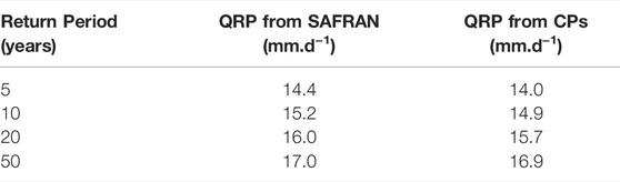
TABLE 5. Comparison between the discharges from a specific return period (QRP) from the historical reference SAFRAN and those from CPs. The latter were obtained from the equation $Q_{spe}=f\left(RP\right)$ established from the mean of the distribution functions of $Q_{max}$ from the 12 CPs.

Evolution of the HIs From CPs in the Future

Figure 5 shows the evolution of the rolling mean in HI classes 1–3 for both the historical and the future CPs under the three RCPs (see Supplementary Figure Appendix SB1 for the graphical results for HI classes 4–5). The results from the Mann–Kendall tests assessing the significance of trends are presented in Table 6. First, all of the HI_{CP_FUTURE} showed strong inter-annual variations but their trends remained relatively linear in most cases from 2006 to 2099. Second, the results showed that the number of changing HIs depended on the RCPs. The annual maximal discharge (5.MaxDisch on Supplementary Figure Appendix SB1 ) and the annual average of peak flow (5.PkFlowAve) were the only two HI_{CP_FUTURE} which changed significantly compared to the HI_{CP_HIST} under all the RCPs: They increased by 2 and 4%, respectively, under RCP2.6, by 9 and 12% under RCP4.5 and by 10 and 16% under RCP8.5. For the remaining HIs from classes 1 to 5, the more pessimistic the RCP, the higher the number of changed HIs.

FIGURE 5

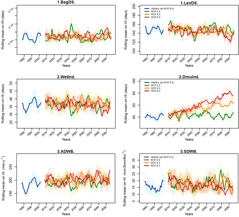
FIGURE 5. Temporal trend of the rolling means of HIs for the first three HI classes “Temporality of the drainage season”, “Water content in the storage” and “Drained water balance” in historical (HI_{CP_HIST}) and future CPs (HI_{CP_FUTURE}) per RCP compared to the rolling means from the historical period. HI names referring to the plots are available in Table 2. For each tick on the x-axis, the value represents the 5-years rolling period centred on this value.

TABLE 6

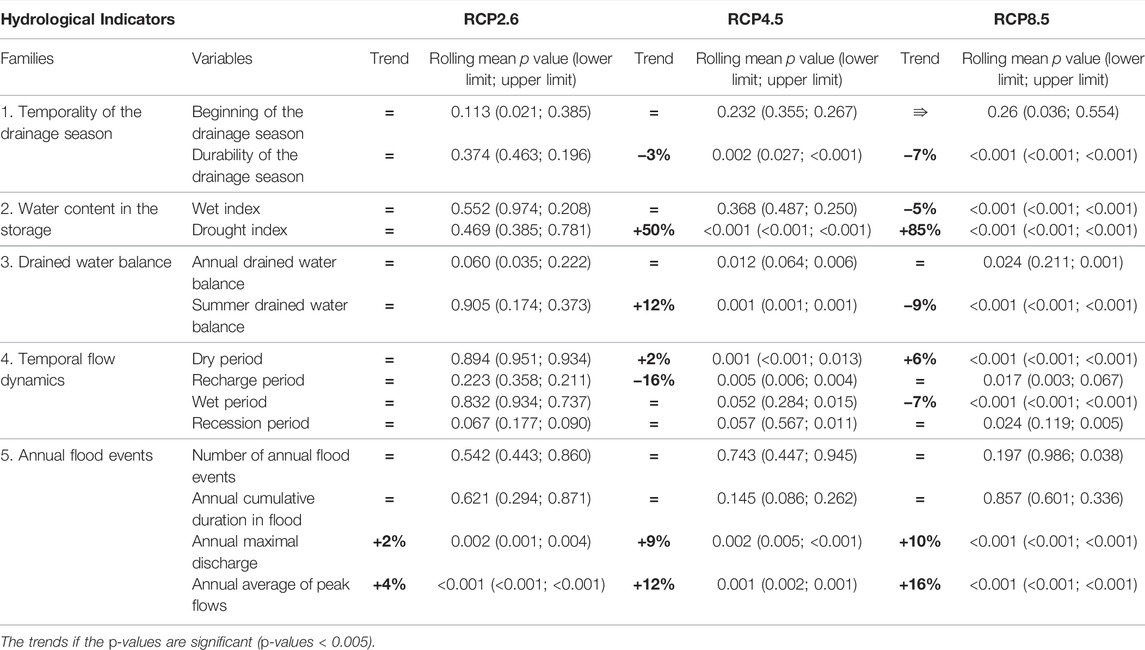
TABLE 6. Results of Mann–Kendall tests regarding the trends from the first five HI classes—“Temporality of the drainage season”, “Water content in the storage”, “Drained water balance”, “Temporal flow dynamics” and “Annual flood events” in the projected future per RCP. Per HI, the p value corresponding to the rolling mean was supported by the p values from the tests on the confidence interval (lower limit; upper limit). The trends were defined as the relative deviation between a mean historical value from 1975–2004 and a mean future value from 2071–2099. Only trends with significant p values were calculated.

Five HI_{CP_FUTURE} started to change from RCP4.5: the summer drained water balance (3.SDWB) increased by 12% and decreased by 9%, respectively, under RCP4.5 and RCP8.5; the drought index (2.DrouInd) increased by 50 and 85%, respectively, under RCP4.5 and RCP8.5; the length of the drainage season (1.LenDS) decreased by 3 and 7%, respectively, under RCP4.5 and RCP8.5; the length of the dry period increased by 2 and 6%, respectively, under RCP4.5 and RCP8.5. According to the Mann–Kendall test, the length of the recharge period (4.LenRechP) was the only HI_{CP_FUTURE} to change under RCP4.5, decreasing by 16%. Finally, two HI_{CP_FUTURE} changed significantly only under RCP8.5: the wet index (2.WetInd) and the length of the wet period (4.LenWetP) both decreased, respectively, by 5% and by 7%.

Some HI_{CP_FUTURE} showed no significant changes under any RCP: the beginning of the drainage season (1.BegDS), the annual drained water balance (3.ADWB), the length of the recession period (4.LenReceP), the annual number of flood events (5.NumFE) and the annual cumulative length in flood (5.CumLenFE). This was congruent with the graphic analysis showing that HI_{CP_FUTURE} had mean values close to the corresponding HI_{CP_HIST}.

An analysis performed on spring flood events, from April to June, showed that the number of spring flood events significantly changed from the historical period to PP3, depending on the RCP (Supplementary Table Appendix SB1). It increased by 43 and 10% under RCP2.6 and RCP4.5, respectively, and decreased by 5% under RCP8.5. The cumulative duration of spring floods started to change under RCP4.5, increasing by 23% and decreasing by 5% under RCP4.5 and RCP8.5, respectively. The average of spring peak flows increased by 12 and 3%, respectively, under RCP4.5 and RCP8.5. Finally, the spring maximal discharge increased only under RCP8.5 by 5%.

The comparison of $Q_{max}$ associated with RPs from CPs between the historical period and PP3 (Table 3), for the three RCPs, revealed that no significant evolution in the future was observed under RCP2.6, with the confidence intervals merging (Figure 6). However, $Q_{max}$ values from the future period were slightly higher than values from the historical period under RCP4.5 and RCP8.5 for PP2 and PP3, with non-superimposing intervals (Figure 6 and Supplementary Figure Appendix SB2). This was consistent with the previous result from HI class 5 showing that the more pessimistic the RCP, the higher the increase of $Q_{max}$. The same applies to the deviations, reaching 4 mm d⁻¹ from the same RP under RCP8.5. The lines in Figure 6 represent the fitted piecewise functions (see Eq. 8) on $Q_{max}$ series from the available CPs per RCP (Table 1).

FIGURE 6

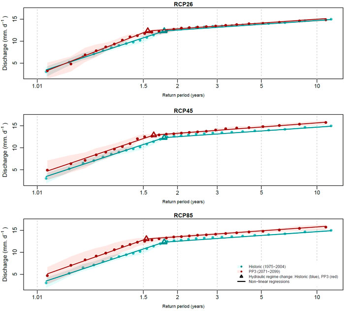
FIGURE 6. Comparison of the specific discharges $Q_{spe}$ (here $Q_{max}$) associated with return periods RPs between the projected future period 2071–2099 (red points) and the projected historical period 1975–2004 (blue points), for the three RCPs. Each scatter plot was calculated from the mean of the distribution functions of $Q_{max}$ from the available CPs according to the corresponding RCP (Table 1), supported by a confidence interval at 95%. The equation $Q_{spe}=f\left(RP\right)$ was fitted as a piecewise function (see Eq. 8) by non-linear regression, for all cases.

Under RCP4.5, those from the future period were higher than the ones from the historical period and the regime change in RC appeared earlier by about 2.7 and 1.8 months, with the corresponding discharge Q_RC increasing by 0.3 and 0.4 mm d⁻¹, respectively, in PP2 and PP3 (Table 7). Regarding RCP8.5, the regime change appeared earlier by 2.5 and 2.9 months, with the corresponding Q_RC values both increasing by 0.5 mm d⁻¹, respectively, in PP2 and PP3. The discharge at the break point from the historical period was reached 4 months earlier by the end of the 21st century, i.e. twice every 3 years instead of once every 2 years.

TABLE 7

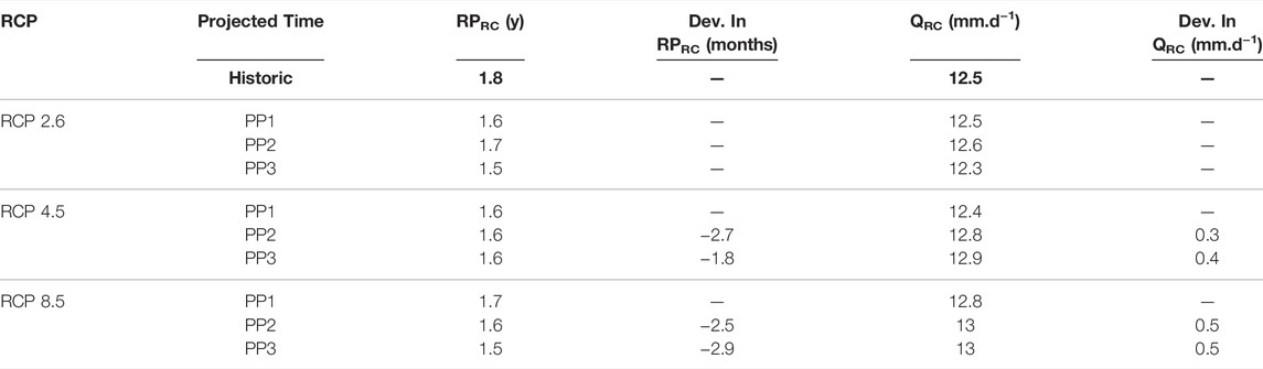
TABLE 7. Evolution of the return period in the regime change RP_RC and the corresponding discharges Q_RC in the projected future for the three RCPs. The deviations (Dev.) for RP_RC and Q_RC were only calculated when the deviations from the historical period to the future were significant, i.e. when the confidence intervals were not superimposed close to the regime change in the graphics.

Figure 7 shows the evolution of the QRP05, QRP10, QRP20 and QRP50 values per RCP and sub-period in the projected time. The associated errors were established using the confidence intervals in the mean distribution function of $Q_{max}$ from CPs. The results showed that no QRP in RCP2.6 varied from the historical period to the future, with the confidence intervals intersecting each other. In PP1, RCP8.5 induced no significant change due to intersecting confidence intervals, whereas RCP4.5 led to an increase in QRP20 and QRP50, respectively, by 0.3 and 0.5 mm d⁻¹. In PP2, neither RCP4.5 nor RCP8.5 induced significant changes in any QRP. In PP3, results showed that under RCP4.5 and RCP8.5, the four QRPs each increased by about 1 mm d⁻¹. There was no significant difference between RCP4.5 and RCP8.5 with regard to intersecting confidence intervals.

FIGURE 7

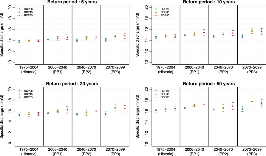
FIGURE 7. Evolution of the QRP05, QRP10, QRP20 and QRP50 values under projected climate. For all situations, i.e. the historical period and the three future sub-periods under the three RCPs, each QRP was calculated from the corresponding fitted piecewise function (see Eq. 8) from the available CPs according to the RCPs (Table 1), and supported by a confidence interval at 95% (bars in the graphics).

Discussion

Impact of the Use of Climate Projections in SIDRA-RU on Hydrological Indicators

In this study, the future of subsurface drainage was assessed feeding the subsurface drainage model SIDRA-RU with climatic projections, resulting in climatic chronicles for a historical period (1975–2004) and a projected period (2006–2100). For HI classes 1–5, we showed that HI_{CP_HIST} and HI_REF trends were not significantly different and were strongly correlated (95%) in most cases. Although the analysis of HI class 6 revealed a possible bias in Eq. 8, it remained negligible as the regime change appeared almost at the same time and with the same specific discharge. Moreover, the QRP05, QRP10, QRP20 and QRP50 values from CPs were similar to those obtained using the observed SAFRAN reanalysis. Consequently, we assumed that bias correction of the indicators was not required to interpret their response under climate change; they have been used for long-term perspectives.

However, some of the deviations observed in extreme values between the HI_{CP_HIST} and the HI_REF, especially for the annual drained water balance, can be questioned. First, we can assume that the deviations arise from the method used to calculate the distribution function of each HI_{CP_HIST}. The latter was extracted from the mean of the distribution functions of the concerned HI from the 12 CPs studied in the historical period under RCP8.5 (Table 1). Consequently, the associated standard deviation was reduced compared to the reference, thus affecting extreme values. Second, the deviations arise from the modelling chain (Figure 2). There are different sources of uncertainty from the estimation of the greenhouse gas emission scenarios to the calculation of HIs, and each stage has its own contribution to the total uncertainty (Vidal et al., 2016; Lemaitre-Basset et al., 2021). The determination of these contributions is a key point in climate change impact studies (Hattermann et al., 2017), which requires further analyses. Third, the deviations arise from the use of the SIDRA-RU model to simulate future discharges. One limitation of the study is that the specific impact of the SIDRA-RU model on the studied HIs was not analysed. One way to analyse it is to extract hydrological indicators from observation (HI_OBS) and to compare them to the HI_REF on the historical period. However, due to significant gaps in observed hydrological data to generate HI_OBS, we were unable to perform such a study. Another way joins the above-mentioned uncertainty analysis from climate components of the modelling chain, consisting of using several hydrological models to relatively establish the contribution of the used hydrological model to the total uncertainty. This will be done in a further study.

Evolution of Subsurface Drainage Under Climate Change

Our results showed that 2–10 out of the 17 HIs studied here were modified under climate change depending on the RCP considered. This change gradually increased as the RCP became more severe and the HIs that changed in a less severe RCP also changed in a more severe RCP: two under RCP2.6 (≈12% of HIs), six under RCP4.5 (≈35% of HIs), 10 under RCP8.5 (≈59% of HIs). This suggests that a very optimistic policy (RCP2.6) does not enable the prevention of all the changes but strongly reduces the number and the magnitude of changes. On the contrary, a policy that does not tackle climate change (RCP8.5, “Business as usual”) causes a larger number of changes in the present-day subsurface drainage in La Jaillière. First, changes appear in flood discharge. Second, the saturation in the storage is impacted, as is the hydraulic saturation of the drainage network. Finally, the temporal flow dynamics and the complete temporality of the drainage season are modified.

The HI showing the strongest change was the drought index, remaining stable under RCP2.6 but increasing significantly from 50% (+20 days) to 85% (+34 days), respectively, under RCPs 4.5 and 8.5 by 2100. This behaviour can be related to the evolution of the other HIs, such as the wet index and the length of the drainage season, both decreasing by approximately 5% under RCP8.5. Similarly, the temporal flow dynamics in the plot was modified, the dry period was longer while the wet period was shorter, by approximately 6% under RCP8.5. These decreases represented an annual 15–30-days longer period of drought. Finally, the summer drained water balance under RCP8.5 by 2100 was reduced by about 10%. All these changes show that drought events are stronger according to how severe the RCP is.

On the other hand, our results showed an intensification of flood events. Indeed, the annual maximal discharge and the annual mean of peak flows were the only HIs to significantly change under all RCPs, with the strongest changes under a pessimistic RCP. Under RCP2.6, this increase was weak, approximately 2–4%. However, it was greater than 10% under RCP8.5. The intensity of flood events influences the regime of hydraulic saturation in the drainage network. Under RCP4.5 and RCP8.5, the regime change appeared 2–3 months earlier, and the same discharge appeared 4 months earlier compared to the historical period. Consequently, under these news conditions, the sustainability and effectiveness of the drainage network could be partially compromised. Moreover, the faster saturation of the drainage network may generate an earlier runoff, which is harmful for crops if the drainage system is less effective in reducing peak flow impacts.

Furthermore, the flood-specific discharge, i.e. the QRP05, QRP10, QRP20 and QRP50, potentially increasing by 2100 by approximately 0.5–1 mm d⁻¹ under RCP4.5 and RCP8.5, respectively, may enhance this effect. Considering that the risk of nitrate leaching during a flood event is highly correlated with the value of the peak flood flow, the increase in the peak flood flow may increase nitrate leaching, especially in winter (Billy et al., 2011; Tournebize et al., 2017). Pesticides, for their part, are less affected by the increase of peak flow in winter, and mostly depend on the interaction between the beginning of the drainage season, which did not change, and the pesticide application (Branger et al., 2009; Delcour et al., 2015). This pertains to most pesticides except for the most mobiles ones, e.g. glyphosate or isoproturon (Le Cor et al., 2021). Moreover, despite RCP8.5 being the most harmful RCP for water quality in winter due to nitrate leaching, our results showed that the frequency of spring flood events increased according to how optimistic the RCP was, changing from three events every 5 years to four to five events every 5 years and being more damaging for pesticide leaching during the main periods of use. The risk is weaker as the scenario becomes pessimistic, most likely correlated with the aforementioned reduction in summer discharge. A pessimistic scenario has a positive effect on water quality in terms of pesticide leaching in spring.

Some HIs did not vary under climate change, such as the beginning of the drainage season. Despite observing stronger flood events, the annual number of flood events and the annual cumulative duration of floods did not change under any RCP, which reinforces the fact that each flood event is stronger under climate change without being longer. The transitory periods from the temporal flow dynamics, i.e. the recharge and recessions periods, did not change either. Although the statistical analyses showed that the recharge period increased under RCP4.5, the increase was approximately 16% (+2 days) which is marginal given the level of uncertainty involved in this analysis cascade. This is reinforced by the fact that the drought index increased while the beginning of the drainage season did not change by 2100, meaning that the soil profile is empty during a longer period but this does not influence its recharge.

Finally, the annual drained water balance does not change under any RCP. This result contradicts the findings from the cited literature that shows either an increase (Pease et al., 2017; Sojka et al., 2020) or a decrease (Dayyani et al., 2012; Mehan et al., 2019; Jiang et al., 2020; Golmohammadi et al., 2021) by the end of the 21st century. Yet, these studies are based on methodologies similar to the one used here: A hydrological model is fed with climate projections simulated from greenhouse gas emission scenarios, mostly RCP4.5 and RCP8.5, to generate future trends. Similarly, four out of these six studies used the DRAINMOD model, including studies with divergent results, excluding the hydrological model effect on the deviation. The deviation therefore more likely arises from the differences in site locations and local climatic or pedologic conditions. This reinforces the point supported in the Introduction about how difficult it is to generalize the impacts of climate change on subsurface drainage. The results of our study are thus limited to the La Jaillière site. To sum up, the results can be used to make general, qualitative projections for the future of subsurface drainage in French sites with similar pedoclimatic contexts, especially the silty sites. However, it is necessary to carry out more precise studies of other drained sites in France to more accurately quantify the impact of climate change on French subsurface drainage.

To summarize, our results show an increase in drought and flood events, which is congruent with the literature predicting an intensification of extreme events such as droughts over France (IPCC, 2014; Marx et al., 2018), and depending on the socio-environmental path our societies follow, some adaptive strategies will be urgently needed. However, the reader has to keep in mind that this study is based on significant assumptions. Among them, current crop is neglected assuming that it does not significantly influence the water balance (see The SIDRA-RU model Section). For example, if the purpose of a future study is to assess the impact of climate change on subsurface drainage from a more agronomic point of view, the SIDRA-RU model does not appear as the wisest choice. This fact limits the emerging interpretations from this study.

Relevant Hydrological Subsurface Drainage Indicators

The major contribution of this study is to introduce 17 HIs to characterize subsurface drainage hydrology. Some HIs already existing in the literature were kept such as the annual drained water balance (Dayyani et al., 2012; Pease et al., 2017; Awad et al., 2020; Wang et al., 2021). To improve the accuracy of the analysis of subsurface drainage, new HIs were set—the length and beginning of the drainage season (Henine et al., 2022); the temporal flow dynamics class distinguishing each annual flow type (Molenat et al., 2008; Humbert et al., 2015; Strohmenger et al., 2020); HIs regarding the water content in the soil storage; HIs dealing with flood events and the discharge specific to an RP (QRP)—which is an approximate version of the indicators currently used to study the impact of climate change on conventional hydrology (Neves et al., 2020; Henriksen et al., 2021). The whole set of HIs allows us to provide farmers and decision-makers with potentially useful tools and information (Kobierska et al., 2020) on crop management, on the risk of pesticide and nitrate leaching and on the sustainability of drainage networks designs.

Each HI informs on a different aspect of subsurface drainage. By assessing the future of 17 HIs (partially independent) instead of one-by-one, our study provides a more integrative understanding of the agrosystem response to climate change. Our study highlights three major possible changes, obviously depending on the scenario that is followed: 1) the increasing intensity of flood events enhances the exposure of crops; 2) this reinforcement also degrades agricultural water quality by favouring the leaching of pollutants; 3) drought events are longer in summer. Considered separately, each of these changes might lead decision-makers to opt for an adaptive strategy that could be inadequate for the other changes. Therefore, understanding the overall and combined impacts of these changes provides a general view of the effects of climate change on subsurface drainage and offers guidance towards the most suitable strategies to adapt to various changes.

Possible Adaptations of Subsurface Drainage to Climate Change

In the “Business as usual” RCP 8.5, the most important changes concern the increase in annual maximal discharge and the peak flows from flood events. Considering the possibly under-dimensioned network of La Jaillière, these changes may result in the faster saturation of pipes and lead to surface runoff potentially damaging current crops. Farmers need to be informed about the risks and potential adaptation options.

One solution to prevent damage to crops from floods is to resize the network by reducing the spacing between drains and/or increasing the pipe diameter. This would increase the rate of water infiltration into the soil, so that the pipes would be filled less quickly thereby reducing the risk of crop-damaging runoff (Broadhead and Skaggs, 1982; Mulqueen, 1998; Nijland et al., 2005). Moreover, this would also reduce the risk of pollutant leaching, which is experienced when high discharges occur shortly after the application period. However, this solution is very expensive and seems difficult to achieve. Drainage system installation on new drained sites may be designed according to these requirements but complementary studies are required to show their efficiency in context of climate change.

Setting retention ponds is another way to prevent damage to crops from flood events (Ferk et al., 2020), to soften the impacts of stronger rainfall events (IPCC, 2014). Set downstream of drained plots, these ponds may also help reduce the leaching of agrochemical inputs (Blankenberg et al., 2007; Tournebize et al., 2012; Tournebize et al., 2017; Vymazal and Březinová, 2015). To be efficient, e.g. cutting 50% of nitrate leaching, the ratio between the pond size and the area of the corresponding drained field must be greater than 2% (Tournebize et al., 2017). Finally, the retention ponds can be useful for saving the excess water in winter from rainfall or direct discharge from the surface drainage network, to be reused for the possible increasing irrigation needs in view of the expected reduction in summer drained water balance under RCP8.5 (Watanabe, 2016; Awad et al., 2020). This strategy was tested in a French context similar to La Jaillière and the ratio of water from winter storage to summer represented 14% of the annual irrigation supplies (Tournebize et al., 2015). However, even if the French government provides financial support to promote and preserve wetlands (Tuffnell and Bignon, 2019), the construction of ponds requires either the allocation of part of the field area, involving a net loss in crop productivity for farmers, or dedicating an equivalent surface connected to the hydraulic network from the drained plot. Both solutions might be troublesome in terms of land management, and therefore such a strategy is inherently challenging to implement in practice.

Instead of adapting the hydraulic dimension of subsurface drainage to climate change, changing agricultural practices can be useful to adapt to its effects. Indeed, the rising frequency of stronger events in a shorter period may increase the number of days of tillage by farmers and then compel them to adapt their agricultural calendar, e.g. to bring forward spring crop sowing. Another solution could be to use crop varieties that grow better in a warmer climate that lead to a decrease in water-holding capacity in summer, e.g. spring crops with a shorter development period, or that are more resilient to flood events (Teixeira et al., 2018) instead of the usual winter wheat and corn. Similarly, shifting the current cultural strategy to more resilient strategies such as crop diversification (Nazir and Das Lohano, 2022) might help to adapt agriculture to the increase in flood events. Changes in tillage practices may also play a role in the adaptation of practices to climate change (Dairon et al., 2017). Further studies are required to validate such proposals. Other less invasive strategies might also be adopted to prevent subsurface drainage from climate change effects, such as numerical tools to help farmers make decisions according to a reasoned use of agrochemicals, e.g. targeting specific times of pesticide supply depending on the season (Lewan et al., 2009; Kobierska et al., 2020).

Conclusion

The aim of this study was to assess the possible future of subsurface drainage under climate change using a large and comprehensive range of hydrological indicators. We first verified that we could use the projected historical hydrological indicators as reference in our subsequent analysis without including critical bias. We then showed that the more pessimistic the scenario of climate change, the more significant the changes in the indicators—a trend that is amplified with time until 2100. Under RCP8.5, the “Business as usual” scenario, the most harmful expected changes are that: 1) the increasing intensity of flood events enhances crop exposure; 2) this reinforcement also deteriorates agricultural water quality by favouring pollutant leaching; 3) drought events are longer in summer. Subsurface drainage will still be usable by 2100, but following the adopted environmental policy, some adaptation strategies are required to best deal with these changes and preserve the environment. However, although the La Jaillière pedology might be a relevant reference for the French drained areas, its climate is location-specific. Analysing the projection of the indicators presented here in other French drained sites subject to different climate conditions and defined by a greater variety of soil types is therefore necessary, thereby allowing for a broader assessment of the future of French subsurface drainage under climate change.

Data Availability Statement

The datasets presented in this article are not readily available because climatic data for this work were provided by Météo-France and are not publicly available since they are part of a commercial product. Météo-France can freely provide them on request for research and non-profit purposes. Requests to access the datasets should be directed to Météo-France, contactmail@meteo.fr.

Author Contributions

AeJ, GT, and JT conceptualized the work. AiJ provided the methodological guidelines on statistical tests. AeJ drafted the paper. GT, AiJ, PM, and JT all revised the paper and contributed to its analyses and discussions.

Funding

This research has been supported by the ANR under the “Investissements d’avenir” programme (Grant Nos. ANR-16-CONV-0003 and CLAND project).

Conflict of Interest

The authors declare that the research was conducted in the absence of any commercial or financial relationships that could be construed as a potential conflict of interest.

Publisher’s Note

All claims expressed in this article are solely those of the authors and do not necessarily represent those of their affiliated organizations, or those of the publisher, the editors and the reviewers. Any product that may be evaluated in this article, or claim that may be made by its manufacturer, is not guaranteed or endorsed by the publisher.

Acknowledgments

We express our gratitude to the Météo-France Meteorological Agency for providing the SAFRAN data and the climate projections from the Euro-Cordex project used in this work. Moreover, we thank the ARVALIS Plant Sciences Institute for providing data from the La Jaillière measurement site. Finally, we want to thank Lila Collet who processed the Euro-Cordex project data to make them usable for this study.

Supplementary Material

The Supplementary Material for this article can be found online at: https://www.frontiersin.org/articles/10.3389/fenvs.2022.899226/full#supplementary-material

References

Abd-Elaty, I., Sallam, G. A. H., Straface, S., and Scozzari, A. (2019). Effects of Climate Change on the Design of Subsurface Drainage Systems in Coastal Aquifers in Arid/Semi-Arid Regions: Case Study of the Nile Delta. Sci. Total Environ. 672, 283–295. doi:10.1016/j.scitotenv.2019.03.483

PubMed Abstract | CrossRef Full Text | Google Scholar

Arnell, N. W., and Gosling, S. N. (2016). The Impacts of Climate Change on River Flood Risk at the Global Scale. Clim. Change 134, 387–401. doi:10.1007/s10584-014-1084-5

CrossRef Full Text | Google Scholar

Arnell, N. W., and Reynard, N. S. (1996). The Effects of Climate Change Due to Global Warming on River Flows in Great Britain. J. Hydrology 183, 397–424. doi:10.1016/0022-1694(95)02950-8

CrossRef Full Text | Google Scholar

Augeard, B., Nedelec, Y., Birgand, F., Chaumont, C., and Ansart, P. (2008). “Effect of a Nonlinear Runoff Response on Flood Statistical Properties : the Case of a Tile-Drained Watershed,” in IAHS-AISH Publication. Presented at the Groundwater-Surface Water Interaction (Process Understanding, Conceptualization and Modelling) Proceedings of Symposium HS1002 at IUGG2007 Perugia, Italy, 124–133.

Google Scholar

Awad, A., Luo, W., and Zou, J. (2021). DRAINMOD Simulation of Paddy Field Drainage Strategies and Adaptation to Future Climate Change in Lower Reaches of the Yangtze River Basin *. Irrig. Drain. 70, 819–831. doi:10.1002/ird.2564

CrossRef Full Text | Google Scholar

Baize, D., and Jabiol, B. (2011). Guide pour la description des sols, Collection Savoir-Faire. Versailles, France: Editions Quae.

Google Scholar

Barrett, T. J., Hille, K. A., Sharpe, R. L., Harris, K. M., Machtans, H. M., and Chapman, P. M. (2015). Quantifying Natural Variability as a Method to Detect Environmental Change: Definitions Of The Normal Range For A Single Observation And The Mean Of M Observations. Environ. Toxicol. Chem. 34, 1185–1195. doi:10.1002/etc.2915

PubMed Abstract | CrossRef Full Text | Google Scholar

Billy, C., Birgand, F., Sebilo, M., Billen, G., Tournebize, J., and Kao, C. (2011). Nitrate Dynamics in Artificially Drained Nested Watersheds. Phys. Chem. Earth, Parts A/B/C 36, 506–514. doi:10.1016/j.pce.2008.09.007

CrossRef Full Text | Google Scholar

Birnbaum, Z. W., and Tingey, F. H. (1951). One-Sided Confidence Contours for Probability Distribution Functions. Ann. Math. Stat. 22, 592–596. doi:10.1214/aoms/1177729550

CrossRef Full Text | Google Scholar

Blankenberg, A.-G. B., Haarstad, K., and Braskerud, B. C. (2007). Pesticide Retention in an Experimental Wetland Treating Non-point Source Pollution from Agriculture Runoff. Water Sci. Technol. 55, 37–44. doi:10.2166/wst.2007.070

PubMed Abstract | CrossRef Full Text | Google Scholar

Bourgin, P. Y., Lobligeois, F., Peschard, J., Andréassian, V., Le Moine, N., Coron, L., et al. (2010). Description des caractéristiques morphologiques, climatiques et hydrologiques de 4436 bassins versants français. Guide d’utilisation de la base de données hydro-climatique (Rapport technique). Antony, France: IRSTEA.

Google Scholar

Boussinesq, J. (1904). Recherches théoriques sur l’écoulement des nappes d’eau infiltrées dans le sol et sur le débit des sources. J. de Mathématiques Pures Appliquées 10, 5–78.

Google Scholar

Branger, F., Tournebize, J., Carluer, N., Kao, C., Braud, I., and Vauclin, M. (2009). A Simplified Modelling Approach for Pesticide Transport in a Tile-Drained Field: The PESTDRAIN Model. Agric. Water Manag. 96, 415–428. doi:10.1016/j.agwat.2008.09.005

CrossRef Full Text | Google Scholar

Broadhead, R. G., and Skaggs, R. W. (1982). Drainage Strategies and Peak Flood Flows. St Joseph, MI: Presented at the Summer Meeting of the American Society of Agricultural Engineers, American Society of Agricultural Engineers ASAE

Google Scholar

Carvalho-Santos, C., Nunes, J. P., Monteiro, A. T., Hein, L., and Honrado, J. P. (2016). Assessing the Effects of Land Cover and Future Climate Conditions on the Provision of Hydrological Services in a Medium-Sized Watershed of Portugal. Hydrol. Process. 30, 720–738. doi:10.1002/hyp.10621

CrossRef Full Text | Google Scholar

Charlton, M. B., and Arnell, N. W. (2014). Assessing the Impacts of Climate Change on River Flows in England Using the UKCP09 Climate Change Projections. J. Hydrology 519, 1723–1738. doi:10.1016/j.jhydrol.2014.09.008

CrossRef Full Text | Google Scholar

Conover, W. J. (1971). Practical Nonparametric Statistics. New York: John Wiley & Sons.

Google Scholar

Córdova, M., Carrillo-Rojas, G., Crespo, P., Wilcox, B., and Célleri, R. (2015). Evaluation of the Penman-Monteith (FAO 56 PM) Method for Calculating Reference Evapotranspiration Using Limited Data. Mt. Res. Dev. 35, 230–239. doi:10.1659/mrd-journal-d-14-0024.1

CrossRef Full Text | Google Scholar

Dairon, R., Dutertre, A., Tournebize, J., Marks-Perreau, J., and Carluer, N. (2017). Long-term Impact of Reduced Tillage on Water and Pesticide Flow in a Drained Context. Environ. Sci. Pollut. Res. 24, 6866–6877. doi:10.1007/s11356-016-8123-x

CrossRef Full Text | Google Scholar

Deelstra, J. (2015). Climate Change and Subsurface Drainage Design: Results from a Small Field-Scale Catchment in South-Western Norway. Acta Agric. Scand. Sect. B - Soil and Plant Sci. 65, 58–65. doi:10.1080/09064710.2014.975836

CrossRef Full Text | Google Scholar

Delcour, I., Spanoghe, P., and Uyttendaele, M. (2015). Literature Review: Impact of Climate Change on Pesticide Use. Food Res. Int. 68, 7–15. doi:10.1016/j.foodres.2014.09.030

CrossRef Full Text | Google Scholar

Dayyani, S., Prasher, S., Madani, A., and Madramootoo, C. (2012). Impact of Climate Change on the Hydrology and Nitrogen Pollution in a Tile-Drained Agricultural Watershed in Eastern Canada. Trans. ASABE 55, 389–401. doi:10.13031/2013.41380

CrossRef Full Text | Google Scholar

Ferk, M., Ciglič, R., Komac, B., and Loczy, D. (2020). Management of Small Retention Ponds and Their Impact on Flood Hazard Prevention in the Slovenske Gorice Hills. Acta Geogr. Slov. 60, 107–125. doi:10.3986/ags.7675

CrossRef Full Text | Google Scholar

FOCUS (2012). FOCUS Surface Water Scenarios in the EU Evaluation Process under 91/414/EEC”. Report of the FOCUS Working Group on Surface Water Scenarios. EC Document Reference SANCO/4802/2001-rev.2. FOCUS. (Revised version SANCO/4802/2001-rev.2).

Google Scholar

Garner, G., Van Loon, A. F., Prudhomme, C., and Hannah, D. M. (2015). Hydroclimatology of Extreme River Flows. Freshw. Biol. 60, 2461–2476. doi:10.1111/fwb.12667

CrossRef Full Text | Google Scholar

Golmohammadi, G., Rudra, R. P., Parkin, G. W., Kulasekera, P. B., Macrae, M., and Goel, P. K. (2021). Assessment of Impacts of Climate Change on Tile Discharge and Nitrogen Yield Using the DRAINMOD Model. Hydrology 8, 1. doi:10.3390/hydrology8010001

CrossRef Full Text | Google Scholar

Grusson, Y., Wesström, I., and Joel, A. (2021). Impact of Climate Change on Swedish Agriculture: Growing Season Rain Deficit and Irrigation Need. Agric. Water Manag. 251, 106858. doi:10.1016/j.agwat.2021.106858

CrossRef Full Text | Google Scholar

Gumbel, E. J. (1954). Statistical Theory of Eextreme Values and Some Practical Applications: A Series of Lectures. Washington DC, United States: U.S. Government Printing Office.

Google Scholar

Hattermann, F. F., Krysanova, V., Gosling, S. N., Dankers, R., Daggupati, P., Donnelly, C., et al. (2017). Cross‐scale Intercomparison of Climate Change Impacts Simulated by Regional and Global Hydrological Models in Eleven Large River Basins. Clim. Change 141, 561–576. doi:10.1007/s10584-016-1829-4

CrossRef Full Text | Google Scholar

Henine, H., Chaumont, C., Tournebize, J., Augeard, B., Kao, C., and Nedelec, Y. (2012). Le rôle des réseaux de drainage agricole dans le ralentissement dynamique des crues : interprétation des données de l’observatoire « Orgeval ». Sci. Eaux Territ. Cahier spécial, 16–23. doi:10.3917/set.hs05.0004

CrossRef Full Text | Google Scholar

Henine, H., Jeantet, A., Chaumont, C., Chelil, S., Lauvernet, C., and Tournebize, J. (2022). Coupling of a Subsurface Drainage Model with a Soil Reservoir Model to Simulate Drainage Discharge and Drain Flow Start. Agric. Water Manag. 262, 107318. doi:10.1016/j.agwat.2021.107318

CrossRef Full Text | Google Scholar

Henine, H., Nédélec, Y., Augeard, B., Birgand, F., Chaumont, C., Ribstein, P., et al. (2010). Effect of Pipe Pressurization on the Discharge of a Tile Drainage System. Vadose Zone J. 9, 36–42. doi:10.2136/vzj2008.0152

CrossRef Full Text | Google Scholar

Henine, H., Nédélec, Y., and Ribstein, P. (2014). Coupled Modelling of the Effect of Overpressure on Water Discharge in a Tile Drainage System. J. Hydrology 511, 39–48. doi:10.1016/j.jhydrol.2013.12.016

CrossRef Full Text | Google Scholar

Henriksen, H. J., Jakobsen, A., Pasten-Zapata, E., Troldborg, L., and Sonnenborg, T. O. (2021). Assessing the Impacts of Climate Change on Hydrological Regimes and Fish EQR in Two Danish Catchments. J. Hydrology Regional Stud. 34, 100798. doi:10.1016/j.ejrh.2021.100798

CrossRef Full Text | Google Scholar

Hipel, K. W., and McLeod, A. I. (1994). “Nonparametric Tests for Trend Detection,” Time Series Modelling of Water Resources and Environmental Systems, Developments in Water Science (Elsevier), 853–938. doi:10.1016/S0167-5648(08)70688-9

CrossRef Full Text | Google Scholar

Hollander, M., and Wolfe, D. A. (1973). Nonparametric Statistical Methods. Ann Arbor, United States: Wiley.

Google Scholar

Humbert, G., Jaffrezic, A., Fovet, O., Gruau, G., and Durand, P. (2015). Dry‐season Length and Runoff Control Annual Variability in Stream DOC Dynamics in a Small, Shallow Groundwater‐dominated Agricultural Watershed. Water Resour. Res. 51, 7860–7877. doi:10.1002/2015wr017336

CrossRef Full Text | Google Scholar

ICID (2021). Agricultural Water Management for Sustainable Rural Development (Annual Report). New Dehli, India: ICID.

Google Scholar

IPCC, F. C. (2014). “Climate Change 2014: Impacts, Adaptation, and Vulnerability. Part A: Global and Sectoral Aspects,”. IPCC. ed, Climate Change 2014: Impacts, Adaptation, and Vulnerability in Contribution of Working Group II to the Fifth Assessment Report of the Intergovernmental Panel on Climate Change (Cambridge, United Kingdom and New York, NY: Cambridge University Press).

Google Scholar

IPCC, F. C. (2008). Technical Paper on Climate Change and Water. I, IPCC. ed. Cambridge, United Kingdom/New York, NY, USA.

Google Scholar

IUSS Working Group WRB (2015). World Reference Base for Soil Resources 2014, Update 2015 International Soil Classification System for Naming Soils and Creating Legends for Soil Maps (Technical Report No. 106). Rome: World Soil Resources ReportsFAO.

Google Scholar

Jacob, D., Petersen, J., Eggert, B., Alias, A., Christensen, O. B., Bouwer, L. M., et al. (2014). EURO-CORDEX: New High-Resolution Climate Change Projections for European Impact Research. Reg. Environ. Change 14, 563–578. doi:10.1007/s10113-013-0499-2

CrossRef Full Text | Google Scholar

Jamagne, M. (1968). Bases et techniques d’une cartographie des sols. Paris, France: Institut National de la Recherche Agronomique.

Google Scholar

Jeantet, A., Henine, H., Chaumont, C., Collet, L., Thirel, G., and Tournebize, J. (2021). Robustness of a Parsimonious Subsurface Drainage Model at the French National Scale. Hydrol. Earth Syst. Sci. 25, 5447–5471. doi:10.5194/hess-25-5447-2021

CrossRef Full Text | Google Scholar

Jiang, Q., Qi, Z., Xue, L., Bukovsky, M., Madramootoo, C. A., and Smith, W. (2020). Assessing Climate Change Impacts on Greenhouse Gas Emissions, N Losses in Drainage and Crop Production in a Subsurface Drained Field. Sci. Total Environ. 705, 135969. doi:10.1016/j.scitotenv.2019.135969

PubMed Abstract | CrossRef Full Text | Google Scholar

Kalantari, Z. (2011). Adaptation of Road Drainage Structures to Climate Change. Stockholm, Sweden: KTH Royal Institute of Technology.

Google Scholar

Khaliq, M. N., Ouarda, T. B. M. J., Gachon, P., Sushama, L., and St-Hilaire, A. (2009). Identification of Hydrological Trends in the Presence of Serial and Cross Correlations: A Review of Selected Methods and Their Application to Annual Flow Regimes of Canadian Rivers. J. Hydrology 368, 117–130. doi:10.1016/j.jhydrol.2009.01.035

CrossRef Full Text | Google Scholar

Kobierska, F., Koch, U., Kasteel, R., Stamm, C., and Prasuhn, V. (2020). Plant Protection Product Losses via Tile Drainage: A Conceptual Model and Mitigation Measures. Agrar. Schweiz 11, 115–123. doi:10.34776/afs11-115

CrossRef Full Text | Google Scholar

Kundzewicz, Z. W., Kanae, S., Seneviratne, S. I., Handmer, J., Nicholls, N., Peduzzi, P., et al. (2014). Flood Risk and Climate Change: Global and Regional Perspectives. Hydrological Sci. J. 59, 1–28. doi:10.1080/02626667.2013.857411

CrossRef Full Text | Google Scholar

Kuzmanovski, V., Trajanov, A., Leprince, F., Džeroski, S., and Debeljak, M. (2015). Modeling Water Outflow from Tile-Drained Agricultural Fields. Sci. Total Environ. 505, 390–401. doi:10.1016/j.scitotenv.2014.10.009

PubMed Abstract | CrossRef Full Text | Google Scholar

Lagacherie, P., and Favrot, J. C. (1987). Synthèse générale sur les études de secteurs de référence drainage. Montpellier, France: INRA.

Google Scholar

Lange, B., Germann, P. F., and Lüscher, P. (2011). Runoff-generating Processes in Hydromorphic Soils on a Plot Scale: Free Gravity-Driven versus Pressure-Controlled Flow. Hydrol. Process. 25, 873–885. doi:10.1002/hyp.7873

CrossRef Full Text | Google Scholar

Le Cor, F., Slaby, S., Dufour, V., Iuretig, A., Feidt, C., Dauchy, X., et al. (2021). Occurrence of Pesticides and Their Transformation Products in Headwater Streams: Contamination Status and Effect of Ponds on Contaminant Concentrations. Sci. Total Environ. 788, 147715. doi:10.1016/j.scitotenv.2021.147715

PubMed Abstract | CrossRef Full Text | Google Scholar

Lebrun, J. D., Ayrault, S., Drouet, A., Bordier, L., Fechner, L. C., Uher, E., et al. (2019). Ecodynamics and Bioavailability of Metal Contaminants in a Constructed Wetland within an Agricultural Drained Catchment. Ecol. Eng. 136, 108–117. doi:10.1016/j.ecoleng.2019.06.012

CrossRef Full Text | Google Scholar

Lemaitre-Basset, T., Collet, L., Thirel, G., Parajka, J., Evin, G., and Hingray, B. (2021). Climate Change Impact and Uncertainty Analysis on Hydrological Extremes in a French Mediterranean Catchment. Hydrological Sci. J. 66, 888–903. doi:10.1080/02626667.2021.1895437

CrossRef Full Text | Google Scholar

Lemaitre-Basset, T., Oudin, L., Thirel, G., and Collet, L. (2022). Unravelling the Contribution of Potential Evaporation Formulation to Uncertainty under Climate Change. Hydrology Earth Syst. Sci. 26, 2147–2159. doi:10.5194/hess-26-2147-2022

CrossRef Full Text | Google Scholar

Lesaffre, B. (1989). Fonctionnement hydrologique et hydraulique du drainage souterrain des sols temporairement engorgés : débits de pointe et modèle SIDRA : extension des principes théoriques de Boussinesq et Guyon. PhD thesis, 6. Paris.

Google Scholar

Lewan, E., Kreuger, J., and Jarvis, N. (2009). Implications of Precipitation Patterns and Antecedent Soil Water Content for Leaching of Pesticides from Arable Land. Agric. Water Manag. 96, 1633–1640. doi:10.1016/j.agwat.2009.06.006

CrossRef Full Text | Google Scholar

Mann, H. B. (1945). Nonparametric Tests Against Trend. Econometrica 13, 245–259. doi:10.2307/1907187

CrossRef Full Text | Google Scholar

Mann, H. B., and Whitney, D. R. (1947). On a Test of whether One of Two Random Variables Is Stochastically Larger Than the Other. Ann. Math. Stat. 18, 50–60. doi:10.1214/aoms/1177730491

CrossRef Full Text | Google Scholar

Marx, A., Kumar, R., Thober, S., Rakovec, O., Wanders, N., Zink, M., et al. (2018). Climate Change Alters Low Flows in Europe under Global Warming of 1.5, 2, and 3 °C. Hydrol. Earth Syst. Sci. 22, 1017–1032. doi:10.5194/hess-22-1017-2018

CrossRef Full Text | Google Scholar

Maurer, E. P., Hidalgo, H. G., Das, T., Dettinger, M. D., and Cayan, D. R. (2010). The Utility of Daily Large-Scale Climate Data in the Assessment of Climate Change Impacts on Daily Streamflow in California. Hydrol. Earth Syst. Sci. 14, 1125–1138. doi:10.5194/hess-14-1125-2010

CrossRef Full Text | Google Scholar

McLeod, A. I. (2011). Kendall Rank Correlation and Mann-Kendall Trend Test, R Package.

Google Scholar

Mechoso, C. R., and Arakawa, A. (2003). “General Circulation | Models,” in Encyclopedia of Atmospheric Sciences. Editor J. R. Holton (Oxford: Academic Press), 861–869. doi:10.1016/B0-12-227090-8/00157-3

CrossRef Full Text | Google Scholar

Mehan, S., Aggarwal, R., Gitau, M. W., Flanagan, D. C., Wallace, C. W., and Frankenberger, J. R. (2019). Assessment of Hydrology and Nutrient Losses in a Changing Climate in a Subsurface-Drained Watershed. Sci. Total Environ. 688, 1236–1251. doi:10.1016/j.scitotenv.2019.06.314

PubMed Abstract | CrossRef Full Text | Google Scholar

Molenat, J., Gascuel-Odoux, C., Ruiz, L., and Gruau, G. (2008). Role of Water Table Dynamics on Stream Nitrate Export and Concentration in Agricultural Headwater Catchment (France). J. Hydrology 348, 363–378. doi:10.1016/j.jhydrol.2007.10.005

CrossRef Full Text | Google Scholar

Moss, R., Babiker, W., Brinkman, S., Calvo, E., Carter, T., Edmonds, J., et al. (2008). Towards New Scenarios for the Analysis of Emissions: Climate Change, Impacts and Response Strategies. Geneva, Switzerland: Intergovernmental Panel on Climate Change Secretariat IPCC.

Google Scholar

Mukundan, R., Hoang, L., Gelda, R. K., Yeo, M.-H., and Owens, E. M. (2020). Climate Change Impact on Nutrient Loading in a Water Supply Watershed. J. Hydrology 586, 124868. doi:10.1016/j.jhydrol.2020.124868

CrossRef Full Text | Google Scholar

Mulqueen, J. (1998). Depth, Spacing and Length of Mole Drains with Applications to Afforestation. Ir. J. Agric. Food Res. 37, 39–49.

Google Scholar

Nam, W.-H., Hayes, M. J., Svoboda, M. D., Tadesse, T., and Wilhite, D. A. (2015). Drought Hazard Assessment in the Context of Climate Change for South Korea. Agric. Water Manag. 160, 106–117. doi:10.1016/j.agwat.2015.06.029

CrossRef Full Text | Google Scholar

Navarro-Racines, C., Tarapues, J., Thornton, P., Jarvis, A., and Ramirez-Villegas, J. (2020). High-resolution and Bias-Corrected CMIP5 Projections for Climate Change Impact Assessments. Sci. Data 7, 7. doi:10.1038/s41597-019-0343-8

PubMed Abstract | CrossRef Full Text | Google Scholar

Nazir, A., and Das Lohano, H. (2022). “Resilience through Crop Diversification in Pakistan,” in Climate Change and Community Resilience: Insights from South Asia. Editors A. K. Enamul Haque, P. Mukhopadhyay, M. Nepal, and M. R. Shammin (Singapore: Springer), 431–442. doi:10.1007/978-981-16-0680-9_28

CrossRef Full Text | Google Scholar

Nedelec, Y. (2005). Interactions en crue entre drainage souterrain et assainissement agricole (phdthesis). Paris, France: ENGREF AgroParisTech.

Google Scholar

Neves, G. L., Barbosa, M. A. G. A., Anjinho, P. d. S., Guimarães, T. T., das Virgens Filho, J. S., and Mauad, F. F. (2020). Evaluation of the Impacts of Climate Change on Streamflow through Hydrological Simulation and under Downscaling Scenarios: Case Study in a Watershed in Southeastern Brazil. Environ. Monit. Assess. 192, 707. doi:10.1007/s10661-020-08671-x

PubMed Abstract | CrossRef Full Text | Google Scholar

Nijland, H., Croon, F., and Ritzema, H. (2005). Subsurface Drainage Practices : Guidelines for the Implementation, Operation and Maintenance of Subsurface Pipe Drainage Systems. Wageningen, Netherlands: Alterra, ILRI Publication.

Google Scholar

Pearson, K., and Galton, F. (1895). VII. Note on Regression and Inheritance in the Case of Two Parents. Proc. R. Soc. Lond. 58, 240–242. doi:10.1098/rspl.1895.0041

CrossRef Full Text | Google Scholar

Pease, L. A., Fausey, N. R., Martin, J. F., and Brown, L. C. (2017). Projected Climate Change Effects on Subsurface Drainage and the Performance of Controlled Drainage in the Western Lake Erie Basin. J. Soil Water Conservation 72, 240–250. doi:10.2489/jswc.72.3.240

CrossRef Full Text | Google Scholar

Potter, N. J., Chiew, F. H. S., Charles, S. P., Fu, G., Zheng, H., and Zhang, L. (2020). Bias in Dynamically Downscaled Rainfall Characteristics for Hydroclimatic Projections. Hydrol. Earth Syst. Sci. 24, 2963–2979. doi:10.5194/hess-24-2963-2020

CrossRef Full Text | Google Scholar

Prudhomme, C., Giuntoli, I., Robinson, E. L., Clark, D. B., Arnell, N. W., Dankers, R., et al. (2014). Hydrological Droughts in the 21st Century, Hotspots and Uncertainties from a Global Multimodel Ensemble Experiment. Proc. Natl. Acad. Sci. U.S.A. 111, 3262–3267. doi:10.1073/pnas.1222473110

PubMed Abstract | CrossRef Full Text | Google Scholar

Prudhomme, C., Wilby, R. L., Crooks, S., Kay, A. L., and Reynard, N. S. (2010). Scenario-neutral Approach to Climate Change Impact Studies: Application to Flood Risk. J. Hydrology 390, 198–209. doi:10.1016/j.jhydrol.2010.06.043

CrossRef Full Text | Google Scholar

R Core Team (2021). R: A Language and Environment for Statistical Computing. Vienna, Austria: R Foundation for Statistical Computing.

Google Scholar

Randall, D., Zehnder, J., and Reviewer, . (2001). General Circulation Model Development: Past, Present, and Future. International Geophysics Series, Vol 70. Int. Geophys. SeriesApplied Mech. Rev. 7054, B94. doi:10.1115/1.1399682

CrossRef Full Text | Google Scholar

Riahi, K., Rao, S., Krey, V., Cho, C., Chirkov, V., Fischer, G., et al. (2011). RCP 8.5—A Scenario of Comparatively High Greenhouse Gas Emissions. Clim. Change 109, 33–57. doi:10.1007/s10584-011-0149-y

CrossRef Full Text | Google Scholar

Saporta, G. (2006). Probabilités, Analyse des données et statistique. Paris, France: Technip.

Google Scholar

Shrestha, S., Bhatta, B., Shrestha, M., and Shrestha, P. K. (2018). Integrated Assessment of the Climate and Landuse Change Impact on Hydrology and Water Quality in the Songkhram River Basin, Thailand. Sci. Total Environ. 643, 1610–1622. doi:10.1016/j.scitotenv.2018.06.306

PubMed Abstract | CrossRef Full Text | Google Scholar

Sojka, M., Kozłowski, M., Kęsicka, B., Wróżyński, R., Stasik, R., Napierała, M., et al. (2020). The Effect of Climate Change on Controlled Drainage Effectiveness in the Context of Groundwater Dynamics, Surface, and Drainage Outflows. Central-western Pol. case study 10, 625. doi:10.3390/agronomy10050625

CrossRef Full Text | Google Scholar

Soubeyroux, J.-M., Bernus, S., Corre, L., Drouin, A., Dubuisson, B., Etchevers, P., et al. (2021). Les nouvelles projections climatiques de référence DRIAS 2020 pour la métropole. Toulouse, France: DRIAS.

Google Scholar

Spearman, C. (1904). The Proof and Measurement of Association between Two Things. Am. J. Psychol. 15, 72–101. doi:10.2307/1412159

CrossRef Full Text | Google Scholar

Strohmenger, L., Fovet, O., Akkal‐Corfini, N., Dupas, R., Durand, P., Faucheux, M., et al. (2020). Multitemporal Relationships between the Hydroclimate and Exports of Carbon, Nitrogen, and Phosphorus in a Small Agricultural Watershed. Water Resour. Res. 56, e2019WR026323. doi:10.1029/2019wr026323

CrossRef Full Text | Google Scholar

Teixeira, E. I., de Ruiter, J., Ausseil, A.-G., Daigneault, A., Johnstone, P., Holmes, A., et al. (2018). Adapting Crop Rotations to Climate Change in Regional Impact Modelling Assessments. Sci. Total Environ. 616, 785–795. doi:10.1016/j.scitotenv.2017.10.247

PubMed Abstract | CrossRef Full Text | Google Scholar

Thompson, J. A., Bell, J. C., and Butler, C. A. (1997). Quantitative Soil-Landscape Modeling for Estimating the Areal Extent of Hydromorphic Soils. Soil Sci. Soc. Am. J. 61, 971–980. doi:10.2136/sssaj1997.03615995006100030037x

CrossRef Full Text | Google Scholar

Thomson, A. M., Calvin, K. V., Smith, S. J., Kyle, G. P., Volke, A., Patel, P., et al. (2011). RCP4.5: a Pathway for Stabilization of Radiative Forcing by 2100. Clim. Change 109, 77–94. doi:10.1007/s10584-011-0151-4

CrossRef Full Text | Google Scholar

Tournebize, J., Chaumont, C., Fesneau, C., Guenne, A., Vincent, B., Garnier, J., et al. (2015). Long-term Nitrate Removal in a Buffering Pond-Reservoir System Receiving Water from an Agricultural Drained Catchment. Ecol. Eng. 80, 32–45. doi:10.1016/j.ecoleng.2014.11.051

CrossRef Full Text | Google Scholar

Tournebize, J., Chaumont, C., and Mander, Ü. (2017). Implications for Constructed Wetlands to Mitigate Nitrate and Pesticide Pollution in Agricultural Drained Watersheds. Ecol. Eng. 103, 415–425. doi:10.1016/j.ecoleng.2016.02.014

CrossRef Full Text | Google Scholar

Tournebize, J., Gramaglia, C., Birmant, F., Bouarfa, S., Chaumont, C., and Vincent, B. (2012). Co-Design of Constructed Wetlands to Mitigate Pesticide Pollution in a Drained Catch-Basin: A Solution to Improve Groundwater Quality. Irrig. Drain. 61, 75–86. doi:10.1002/ird.1655

CrossRef Full Text | Google Scholar

Tuffnell, F., and Bignon, J. (2019). Terres d’eau, terres d’avenir : “Faire de nos zones humides des territoires pionniers de la transition écologique” (Final report). Paris: French National Assembly & French Senat.

Google Scholar

Tuohy, P., O’ Loughlin, J., Peyton, D., and Fenton, O. (2018). The Performance and Behavior of Land Drainage Systems and Their Impact on Field Scale Hydrology in an Increasingly Volatile Climate. Agric. Water Manag. 210, 96–107. doi:10.1016/j.agwat.2018.07.033

CrossRef Full Text | Google Scholar

van Vuuren, D. P., den Elzen, M. G. J., Lucas, P. L., Eickhout, B., Strengers, B. J., van Ruijven, B., et al. (2007). Stabilizing Greenhouse Gas Concentrations at Low Levels: an Assessment of Reduction Strategies and Costs. Clim. Change 81, 119–159. doi:10.1007/s10584-006-9172-9

CrossRef Full Text | Google Scholar

Verfaillie, D., Déqué, M., Morin, S., and Lafaysse, M. (2017). The Method ADAMONT v1.0 for Statistical Adjustment of Climate Projections Applicable to Energy Balance Land Surface Models. Geosci. Model Dev. 10, 4257–4283. doi:10.5194/gmd-10-4257-2017

CrossRef Full Text | Google Scholar

Vidal, J.-P., Hingray, B., Magand, C., Sauquet, E., and Ducharne, A. (2016). Hierarchy of Climate and Hydrological Uncertainties in Transient Low-Flow Projections. Hydrol. Earth Syst. Sci. 20, 3651–3672. doi:10.5194/hess-20-3651-2016

CrossRef Full Text | Google Scholar

Vidal, J.-P., Martin, E., Franchistéguy, L., Baillon, M., and Soubeyroux, J.-M. (2010). A 50-year High-Resolution Atmospheric Reanalysis over France with the Safran System. Int. J. Climatol. 30, 1627–1644. doi:10.1002/joc.2003

CrossRef Full Text | Google Scholar

Vymazal, J., and Březinová, T. (2015). The Use of Constructed Wetlands for Removal of Pesticides from Agricultural Runoff and Drainage: A Review. Environ. Int. 75, 11–20. doi:10.1016/j.envint.2014.10.026

PubMed Abstract | CrossRef Full Text | Google Scholar

Wang, Z., Zhang, T. Q., Tan, C. S., Xue, L., Bukovsky, M., and Qi, Z. M. (2021). Modeling Impacts of Climate Change on Crop Yield and Phosphorus Loss in a Subsurface Drained Field of Lake Erie Region, Canada. Agric. Syst. 190, 103110. doi:10.1016/j.agsy.2021.103110

CrossRef Full Text | Google Scholar

Watanabe, T. (2016). How Do Irrigation and Drainage Play an Important Role in Climate Change Adaptation? Irrig. Drain. 65, 189–196. doi:10.1002/ird.1980

CrossRef Full Text | Google Scholar

Xu, X., Wang, Y.-C., Kalcic, M., Muenich, R. L., Yang, Y. C. E., and Scavia, D. (2019). Evaluating the Impact of Climate Change on Fluvial Flood Risk in a Mixed-Use Watershed. Environ. Model. Softw. 122, 104031. doi:10.1016/j.envsoft.2017.07.013

CrossRef Full Text | Google Scholar

Yin, J., Yu, D., Yin, Z., Liu, M., and He, Q. (2016). Evaluating the Impact and Risk of Pluvial Flash Flood on Intra-urban Road Network: A Case Study in the City Center of Shanghai, China. J. Hydrology 537, 138–145. doi:10.1016/j.jhydrol.2016.03.037

CrossRef Full Text | Google Scholar

Zhang, Y., Wang, Y., Chen, Y., Liang, F., and Liu, H. (2019). Assessment of Future Flash Flood Inundations in Coastal Regions under Climate Change Scenarios-A Case Study of Hadahe River Basin in Northeastern China. Sci. Total Environ. 693, 133550. doi:10.1016/j.scitotenv.2019.07.356

PubMed Abstract | CrossRef Full Text | Google Scholar