A case analysis of turbulence characteristics and ozone perturbations over eastern China

Our knowledge of the vertical variabilities in turbulence and ozone perturbation in the free atmosphere is severely limited because of the scarcity of high-resolution observation data. Based on the Thorpe method, a new set of sounding data in Shanghai, China, was used herein to analyze the distributions of turbulence and ozone perturbation. The region in which turbulence activity is relatively frequent spans from 5-15 km in the middle and upper troposphere. Due to the combined action of large wind shear and thermal convection, the low-troposphere stratification conditions are conducive to the generation of large-scale turbulence. Turbulence has a certain effect on atmospheric ozone concentration exchanges; in most regions located near turbulence, ozone partial pressure perturbations occur. In the troposphere, the ozone profile is most influenced by atmospheric static instability, while in the stratosphere, both wind shear and thermal convection play important roles in the emergence of ozone perturbations.

Introduction

Turbulence is a disturbance phenomenon that occurs in the vertical direction and plays a crucial role in global dynamic meteorology. The generation of turbulence can affect the momentum and energy budgets as well as the exchange and transfer of gas in the free atmosphere (Lobken 1992; Fritts et al., 2012). Turbulence is also well-known harmful to aviation, as it is the main cause of aircraft jolting and has caused many injuries in recent years (Sharman et al., 2012). In addition, turbulence can heat the atmosphere through molecular dissipation and cool it through heat con-duction (Zhao et al., 2019). The kinetic energy dissipation rate associated with turbulence reflects the rate of the heat budget and is an important parameter indicating the turbulence intensity. Many factors affect turbulence, such as solar radiation, latent heat release and atmospheric chemistry. The breaking of gravity waves generates turbulence under unstable atmospheric conditions (Miyazaki et al., 2010; Xu et al., 2017). The large wind shears that occur at the tropopause and their interactions with turbulence have also been studied in the past (Sunilkumar et al., 2015).

As turbulence is a small-scale perturbation process, it is important to observe this phenomenon accurately. Various observation techniques have been developed during the last few years for estimating turbulence parameters, such as in situ detection methods with probes mounted on rockets and aircraft (Cho et al., 2003; Dehghan, Hocking, and Srinivasan 2014) and remote sensing technologies that involve the use of satellites and radars (Hocking 1988; Lobken 1992; Nastrom and Eaton 1997; Singh et al., 2008). However, rockets and aircraft provide data only on specific routes, and the associated costs are high (Cohn 1995). Radar detection can provide continuous observations but are confined to the location of the utilized radar and can cover only a small part of the atmosphere (Singh et al., 2008). When compared with radar and rocket detection methods, radiosonde data can cover most areas and make continuous observations, allowing turbulence parameters to be better calculated. Thorpe first proposed a method for estimating the turbulence mixing layer in the ocean, providing a good reference for the field of meteorology. Clayson and Kantha (2008) proved the feasibility of the Thorpe analysis method in the atmosphere using a large amount of radiosonde data to detect local turbulence and estimate the energy dissipation rate and eddy diffusivity (Clayson and Kantha 2008). Kantha and Hocking (2011) combined the turbulent kinetic energy dissipation rate (ε) calculated from stratosphere-tropospheric (ST) radar with that derived from radiosonde rata and proved that the above two results have good consistency (Kantha and Hocking 2011). Wilson et al. (2010, 2013) pointed out the effects of instrument noise and air moisture on the Thorpe method results and improved it correspondingly (Wilson et al., 2010, 2013). At present, the Thorpe meth-od has been widely used to extract turbulent layers from sorted potential temperature profiles.

Ozone has a crucial impact on the thermal components and structure of the global atmosphere (Xia, Huang, and Hu 2018; Chang et al., 2020). Ozone variations in the atmosphere are controlled by thermal, dynamic and chemical processes. These factors act individually or mutually to induce ozone feedbacks, which often manifest as the denaturation of the atmospheric vertical structure and affect the climate and ecological environment (Xia et al., 2018; Wang, Wang, and Wang 2020). Ozone not only determines the existence of the stratosphere but also modulates the amount of solar radiation that reaches the ground and affects the radiation budget of the Earth-atmosphere system (Ramaswamy et al., 2001). Tropospheric ozone has strong radiative forcing and greenhouse climate effects (Maleska, Smith, and Virgin 2020; Zhang et al., 2022), and high near-ground ozone contents seriously harm human health. The stability of ozone in the atmosphere has thus been an area of great concern. Since 1985, when the Antarctic ozone hole was discovered for the first time, globally relevant scientific workers have paid great attention to changes in the ozone content in the atmosphere. Xie et al. (2014) pointed out that El Niño Southern Oscillation (ENSO) has a strong influence in the ozone. The El Niño events can lead to a decrease of ozone in the lower-middle stratosphere. Higher total ozone column (TOC) is also found over most parts of China during those events (Xie et al., 2014; Zhang et al., 2015). Chang et al. (2020) pointed out the response of ozone to gravity waves and showed that when gravity waves break, high stratospheric ozone contents in the stratosphere are injected into the troposphere (Ramaswamy et al., 2001)(Ramaswamy et al., 2001)(Ramaswamy et al., 2001). Ozone perturbations can also obviously influence the high cloud fraction through extensive experimentation. Zhang et al. (2019) also analyzed the zonally asymmetric trends of TOC in the northern middle latitudes in winter (Jiankai et al., 2019). The effective detection of the ozone vertical profile can provide vital information regarding the control mechanism of the ozone layer state and for the study of ozone climate effects. At present, telemetry has been used for many years to invert ozone vertical profiles (Jackman et al., 1989; Chan et al., 2000; Pierazzo et al., 2010; Yang et al., 2017), but today, due to relatively large ozone variabilities and poor detection data, high uncertainties exist in ozone perturbation research, and available ozone sonde data are very scarce.

In this paper, we use a set of radiosonde data to analyze the turbulence and ozone perturbation conditions over east China by the Thorpe method, thus filling in the research gap in this research. The main contents of this paper are organized as follows. Section 2 describes the utilized radiosonde datasets. Section 3 describes the principle of the Thorpe method and the calculations of the turbulence parameters. Section 4 analyzes the spatial distributions of the turbulence parameters. Section 5 analyzes the relationship between turbulence and ozone perturbations. Section 6 presents a summary and conclusions.

Data

Our team totally obtained 6 sets of data points in the Baoshan area of Shanghai and 5 sets of unabridged atmospheric profiles recorded from October 15 to 21 October 2021. The specific data information is provided in Table 1. Based on a newly available ozone-detection instrument and Beidou positioning technology, the atmospheric temperature, pressure, ozone, wind speed and direction were measured. The radial and zonal winds are calculated from the wind speed and direction data. Compared with the previously utilized detection instrument, the accuracy of this novel system has been improved. The mean vertical resolution is 6 m. In this study, cubic spline interpolation is used to fit the data profiles to facilitate simple calculations.

TABLE 1

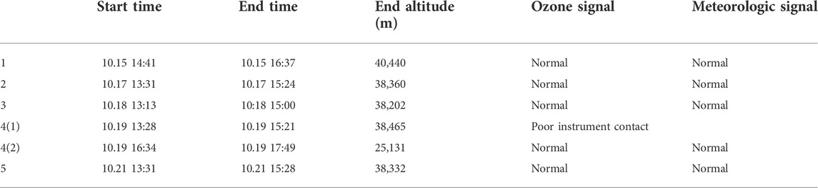
TABLE 1. Information of sounding data collected over Shanghai from October 15 to 21 October 2021.

The normal signal points that the profiles have no missing ozone, pressure, temperature, relative humidity, and wind data between successive data. Table 1 shows that the data collected from 13:23 on October 19 were lost due to wrong signal caused by poor instrument contact. In addition, no data were available on October 16 or 20 due to rain. All of the rest of the collection periods exhibit good effects, and the ozone and meteorologic signals are normal. The maximum flight altitude is 40,440 m, and the minimum flight altitude is 25,131 m.

Methods

Calculation of the turbulence and ozone parameters

The potential temperatures calculated from the original pressure, temperature and humidity (PTU) data always monotonically increased under statically stable atmospheric conditions, but local regions exhibited overturns due to various scales of turbulence. Thorpe (1977) devised a straightforward means to estimate the scale of these inversions in a stratified fluid; this method consists of reordering the detected potential temperature profile into a monotonic profile without overturns (Thorpe 1977). The difference between the values generated before and after this sorting is the Thorpe displacement value. Supposing that a sample observed at an altitude $Z_n$ needs to be moved to the altitude of $Z_m$ after sorting, the resulting value is the so-called the Thorpe displacement:

${\mathit{D}}_{\mathit{n}}=\left|{\mathit{z}}_{\mathit{m}}-{\mathit{z}}_{\mathit{n}}\right|$

The Thorpe scale ($L_T$) is calculated by obtaining the root mean square value of the displacement. $L_T$ shows the local overturning scale in the atmosphere column (Crawford, 1986; Riley and Erik, 2008) and is related to the Ozmidov scale ($L_0$), which describes turbulence in a stably stratified fluid and can be expressed as follows (He et al., 2020b):

${\mathit{L}}_0={\left(\mathit{\epsilon }/{\mathit{N}}^{\mathbf{3}}\right)}^{\mathbf{1}/\mathbf{2}}$

where ε is the turbulent dynamic energy dissipation rate and N is the background Brunt-Vaisala frequency, as estimated from the sorted monotonic potential temperature to eliminate the distribution of turbulence. The relationship between $L_0$ and $L_T$ can be expressed as ${\mathit{L}}_0=\mathit{c}{\mathit{L}}_{\mathit{T}}$ (Gavrilov et al., 2005), and ε can be calculated from $L_T$ as follows:

$\mathit{\epsilon }={\mathit{C}}_{\mathit{k}}{\mathit{L}}_{\mathit{T}}^{\mathbf{2}}{\mathit{N}}^{\mathbf{3}}$

where ${\mathit{C}}_{\mathit{k}}={\mathit{c}}^{\mathbf{2}}$ and c is an empirical constant. Clayson chose ${\mathit{C}}_{\mathit{k}}$ = 0.3 based on his own measurements and judgment and achieved good results. In this paper, ${\mathit{C}}_{\mathit{k}}$ = 0.3 is also used to calculate ε based on the previous studies. (Clayson and Kantha 2008; He et al., 2020a; Qin et al., 2022).

Atmospheric ozone variations are controlled by dynamic, radiative and chemical processes. In this study, the vertical ozone partial pressure gradient is used to represent ozone perturbations. The ozone partial pressure was first interpolated to a vertical height profile of 6 m, and the vertical decline rate was calculated. When ozone perturbation occurs, the local change rate of ozone partial pressure in the vertical di-rection changes dramatically. To express the rate of this change, the absolute value of the change rate of the ozone gradient was calculated; the larger the absolute value of this term was, the faster the change in ozone was, and the stronger the ozone perturbation was.

Noise removal

The principle of the Thorpe method involves finding the inversion regions in which the potential temperature decreases with altitude. However, in the real atmosphere, these regions can be caused not only by real turbulence; other factors such as the exit of noise can also induce elemental overturning and is unavoidable. Wilson et al., 2011. Pointed out that when using low-resolution detection data (5–9 m), only 7.9% of the potential temperature inversion results were selected as real turbulence, and the rest of the results were deemed to be noise and removed (Wilson et al., 2011). Therefore, it is necessary to remove the noise caused by false potential temperature inversions when calculating the turbulent parameters, and this task has an important influence on the Thorpe method. According to the study of Gavrilov et al. (Crawford, 1986; Gavrilov et al., 2005), the following steps can be used to calculate the temperature, pressure and ozone noises. First, the sample data are divided into segments by length (in this paper, we selected 180 m as a segment), and then a linear fit is performed on each segment. The residual is then calculated by obtaining the first-order difference between the sample data and the fitted data, and the noise variance is calculated as half of the residual variance. Finally, the standard deviation of noise can be expressed as the root mean square of the noise variance. For an initial potential temperature profile, the magnitude of the false inversion caused by noise is dependent on the noise level, vertical resolution, and atmospheric stratification state (Wilson et al., 2011). To study the level of instrument-induced noise on the potential temperature values, the bulk trend noise ratio (TNR) is introduced herein (Wilson et al., 2010); For a given profile, the utilized formula of bulk TNR can be expressed as follows:

$\overline{\xi }=\frac{{\mathbf{\theta }}_{\mathbf{n}}-{\mathbf{\theta }}_1}{\left(\mathbf{n}-1\right){\mathbf{\sigma }}_{\mathbf{\theta }}}$

where n is the number of samples in the local region and ${\text{σ}}_{\text{θ}}$ is the noise standard deviation of the potential temperature. The term ${\text{σ}}_{\text{θ}}$ can be calculated using the error transfer formula ${\text{σ}}_{\text{θ}}=\text{θ}\sqrt{{\left(\frac{{\sigma }_t}{T}\right)}^2+{\left(\frac{2{\sigma }_P}{7P}\right)}^2}$, where ${\text{σ}}_{\text{T}}$ and ${\sigma }_P$ are the standard deviation of the temperature and pressure noise. $\overline{\text{ξ}}$ shows that the size of the bulk TNR is influenced by the resolution and noise standard deviation. The larger the noise standard deviation in a particular region is, the smaller ζ value is. A response threshold must be set to screen regions in which the instrumental noise is high (in this paper, we used 0.8 as the threshold). The bulk TNR of troposphere and stratosphere are calculated respectively. For regions in which the TNR is less than 0.8, the potential temperature will be smoothed and sampled with two window to reduce the data resolution and improve the resulting TNR values. When observing the regions in which the ozone perturbation is strong, the ozone data are also smoothed and sampled to calculate the gradient of ozone and, thus, reduce the influence of noise.

In addition, Wilson et al. (2010) proposed a method for selecting the turbulence-induced overturns among all overturns in a dataset. This method involves performing statistical tests on the results. The ${\text{W}}_{\text{θ}}\left(\text{n}\right)={\text{θ}}_{\text{max}}-{\text{θ}}_{\text{min}}$ signal is calculated herein from the potential temperature flip, where n is the number of samples in the flipping area. $W_{95}\left(n\right)$ is calculated through a Monte Carlo simulation, which represents the 95 percentiles of the n independent, identically distributed variables. Comparing the $W_{\theta }\left(n\right)$ signals with $W_{95}\left(n\right)$, when the inverted signal satisfies $W_{\theta }\left(n\right)$ < ${\sigma }_{\theta }{W}_{95}\left(n\right)$, the signal is considered to be caused by noise and is thus removed (Wilson et al., 2010; He et al., 2021).

Results

Atmospheric basic elements contain considerable background information, which can serve as an important means when analysing turbulence. In this paper, 5 datasets collected in Baoshan, Shanghai, from October 15 to 21, 2021, are used to study the local atmospheric turbulence and ozone perturbation conditions. The basic elements of these 5 datasets are shown in Figure 1.

FIGURE 1

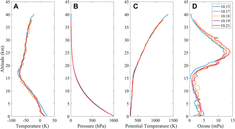
FIGURE 1. Atmospheric background elements recorded from October 15 to 21, 2021: (A) temperature; (B) pressure; (C) potential temperature; and (D) ozone partial pressure.

Figure 1 shows the temperature, air pressure, potential temperature and ozone partial pressure data recorded from October 15 to 21 October 2021. Figure 1A shows the temperature distribution. The tropopause height is determined by the cold point method. (Wang et al., 2019). The average minimum temperature of the five data sets is 16.8 km; this height is thus regarded as the boundary between the troposphere and stratosphere in this paper. Figure 1B shows the distribution of pressure, the five groups of data have good consistency. Figure 1C shows the vertical profile of the potential temperature, which increased monotonously with altitude overall; this phenomenon is the basis of the Thorpe method. However, some small perturbations can be observed in the overall monotonic trends when zooming to the viewport in the profiles, and these perturbations are thought to be caused by turbulence and instrumental noise. Figure 1D shows the ozone partial pressures recorded in the 5 datasets; these values are generally small in the troposphere, and the low-value ranges can be observed at heights of approximately 14-15 km. The average value and average height of the minimum ozone partial pressures are 10.9 mPa and 14.55 km, respectively; this height is below the tropopause height. The maximum ozone layer is recorded at approximately 25 km, and the maximum ozone partial pressure is 13.18 mPa. These results are the same as those observed by Wang et al. (Wang, 2004). It can also be seen from Figure 1D that the same as the profile of potential temperature, some small ozone perturbations can be observed in the vertical direction.

To determine the real turbulence and ozone perturbations in the atmosphere rather than noise, the standard deviations of the temperature, pressure, potential temperature and ozone noise values recorded on October 15 are shown in Figure 2. The red lines denote the moving averages of the raw data and are included only for convenient visualization. Due to the good consistency of the five datasets, only 1 day’s noise distribution is shown here.

FIGURE 2

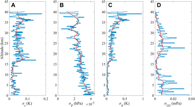
FIGURE 2. Noise standard deviations of (A) temperature, (B) pressure, (C) potential temperature and (D) ozone partial pressure recorded on 15 October 2021.

As seen from Figure 2A, the ${\sigma }_T$ values are generally lower than 0.1 K, and the relatively large values are approximately in the stratosphere, which may have been caused by the limitations on the detection height of the temperature sensor itself (He et al., 2020a). Figure 2B shows the vertical profile of ${\sigma }_P$, the values of which are below 0.004 hPa and decrease with altitude. The distribution of ${\sigma }_{\theta }$ shown in Figure 2C is calculated from the P and ${\sigma }_T$ values and is generally small in the troposphere and increased at approximately 15 km due to the relatively high ${\sigma }_T$ values at this height. Above the altitude of 30 km, another rise in ${\sigma }_{\theta }$ can be observed; according to the error transfer formula, this rise is thought to be caused by the relatively low pressure. Figure 2C shows that because of the relatively high ${\sigma }_{\theta }$, the turbulences above 30 km are not to be considered in this analysis because of the strong mixing of real turbulence and noise at that altitude. Figure 2D shows the vertical profile of ${\sigma }_{ozone}$, which is similar to the distribution of the ozone partial pressure. Relatively large values are observed at approximately 5 km and 25 km, the Ozone data above 30 km is not available, because the pump efficiency is not enough.

Figure 3 shows the distributions of the Brunt-Vaisala frequency, wind shear, and Richardson number on 15 October 2021, reflecting the background stability conditions of the atmosphere; the red lines in the figure represent the moving average of the raw data and are the same as the above Figure 2, which are included for visualization purposes. $N^2$ can be used to characterize the motion states of air particles in the atmosphere. According to Wilson’s study, N is strongly influenced by the presence of water vapor, so we divide this value into the wet Brunt-Vaisala frequency ($N_m$) and the dry Brunt-Vaisala frequency ($N_d$) based on the relative threshold method (Zhang et al., 2010; Wilson et al., 2013). When $N^2<0$, the atmosphere is influenced by convection and is in a static unstable state. Wind shear describes the shear instability in a stratified atmosphere and can be calculated as follows:

$\mathit{Shear}=\sqrt{{\left(\frac{\mathbf{\partial }\overline{\mathbf{u}}}{\mathbf{\partial }\mathbf{z}}\right)}^{\mathbf{2}}+{\left(\frac{\mathbf{\partial }\overline{\mathbf{v}}}{\mathbf{\partial }\mathbf{z}}\right)}^{\mathbf{2}}}$

where ∆z = 6 m, u and v are zonal and meridional winds respectively. Corresponding to the vertical resolution of the data. Large wind shear is a crucial source of shear instability. When the wind shear is large, conditions are favorable for the shear force to exert work, and this process an important factor affecting turbulence (Zhang et al., 2019; He et al., 2020a). The Richardson number can be calculated as follows:

$\mathit{Ri}=\frac{\overline{{\mathbf{N}}^{\mathbf{2}}}}{{\left(\mathbf{\partial }\overline{\mathbf{u}}/\mathbf{\partial }\mathbf{z}\right)}^2+{\left(\mathbf{\partial }\overline{\mathbf{v}}/\mathbf{\partial }\mathbf{z}\right)}^{\mathbf{2}}}$

FIGURE 3

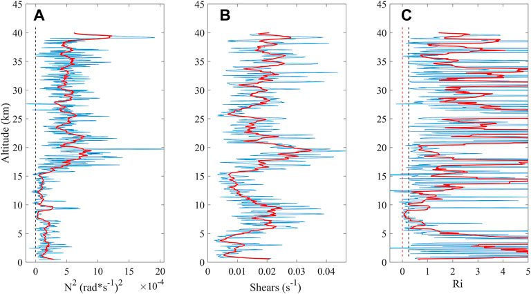
FIGURE 3. Vertical profiles of (A) $N^2$, (B) wind shear, and the (C) Richardson number on 15 October 2021; the red lines denote the moving averages of the raw data.

Ri is an important parameter used to measure the instability of the atmosphere, and the critical values of Ri are 0 and 0.25; these values denote the boundaries of dynamic and static instabilities, respectively (Fritts and Joan Alexander, 2003).

Figure 3A shows the $N^2$ distribution; the black dotted line denotes the critical value of 0. The figure shows that $N^2$ is generally small in the troposphere and is below $3\times {10}^{-4}$ ${\left(rad\ast s^{-1}\right)}^2$; the minimum-value region occurs in the upper troposphere, where the air particles are strongly influenced by convection and are in a state of static instability. In the stratosphere, as the stability increases rapidly, $N^2$ is generally large; negative $N^2$ values are observed at only a few heights. As shown in Figure 3B, the wind shear at altitudes of 10-15 km is generally large; with increasing height, another maximum is found at approximately 17 km due to the existence of the jet stream near the tropopause, both of which bring considerable shear instability. It should be noted that at an altitude of approximately 3 km, a maximum wind shear value is observed, which is beneficial to the generation of turbulence. Figure 3C shows the vertical profile of the Richardson number. The red dotted line represents the boundary of static instability, and the black dotted line denotes the boundary of dynamic instability. Matched with the wind shear and Brunt-Vaisala frequency distributions, Figure 3C shows that a negative Ri value existed at approximately 3 km due to the relatively high wind shear and low $N^2$ value. At altitudes of approximately 5-10 km, in the layer of maximum wind shear, Ri was generally between 0 and 0.25, suggesting the presence of strong dynamic instability at these heights. Corresponding to the lowest $N^2$ values, a region with considerable static instability is observed in the upper troposphere at approximately 10-15 km. In the stratosphere, Ri is generally high, and the atmosphere is stable; these conditions are not conducive to the generation of turbulence.

The inversion of the potential temperature is used herein to calculate the turbulence parameter, and the results are shown in Figure 4. The Thorpe scale ($L_T$) reflects the degree of potential temperature reversal and is used in this work to measure the strength of turbulence. The thickness of the turbulence layer reflects the vertical scale of the turbulence. Since the highest standard noise deviation of the potential temperature above 30 km, the turbulence at this altitude is regarded as an inversion caused by instrument noise and is thus ignored. As the Thorpe analysis cannot distinguish between convective-induced turbulence and shear-induced turbulence, the turbulence estimated using the Thorpe method can be overestimated near the surface during the daytime. Because of this, only “free atmosphere” turbulences above 2 km are considered.

FIGURE 4

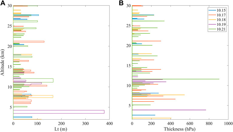
FIGURE 4. Distributions of the (A) Thorpe scale and (B) thickness of the turbulence layer from October 15 to 21, 2021.

Figure 4A, which exhibits the $L_T$ distribution, shows that turbulence occurred more frequently in the troposphere than in the stratosphere. The stability of the stratospheric atmosphere is strong, mainly manifested in high $N^2$ values that is not beneficial to the generation of turbulence. The highest tropospheric turbulence frequency is identified at heights of 10-15 km. Corresponding to Figure 3, the smallest $N^2$ value occurs at this height, and Ri value is less than 0. Because of the shear instability caused by the large wind shear, there is also an area in which turbulence occurs frequently at 5-10-km heights. In addition, a small $N^2$ value is identified in the low troposphere, where the wind shear is large. Under these conditions, thermal convection and shear force work together to create an environment that is conducive to the generation of large-scale turbulence. As shown in the figure, the largest turbulence occurs at 3.7 km on October 19, whose $L_T$ is 378.3 m; the thicknesses corresponding to these values are also maintained at high levels, at 768 m. The distribution of the turbulent layer thickness shown in Figure 4B is similar to that of $L_T$ shown in Figure 4A, and the thickest turbulence is identified in the upper troposphere, reaching 906 m. The turbulence zones with relatively large $L_T$ values are also generally has relatively thick.

To better see the relevant characteristics at different heights, the turbulence is divided into four groups according to altitude: low-troposphere turbulence at 2-5 km, middle-troposphere turbulence at 5-10 km, upper-troposphere turbulence at 10-16.8 km and lower stratosphere turbulence at 16.8-30 km. The turbulence number density, maximum $L_T$ value and other characteristics are calculated for these four groups and are listed in Table 2. The turbulence number density refers to the average amount of turbulence measured per kilometer of altitude.

TABLE 2

TABLE 2. Turbulence number density, maximum Thorpe scale and other characteristics of the 4 turbulence groups.

Table 2 shows that the distributions of turbulence at different altitudes are consistent with the findings obtained from the previous analysis. The turbulences in the low-troposphere region are generally large, with the max $L_T$ value reaching 378 m and the max thickness value reaching 768 m. The mean $L_T$ and thickness values are also much larger for this group than for the others. The turbulence number density measured in the middle troposphere is 3.2; The maximum $L_T$ value reaches 165 m, and the maximum turbulence thickness reaches 546 m. Turbulence occurs most frequently in the upper troposphere; here, the average amount of turbulence per kilometer reaches 3.5, which is also beneficial to the emergence of relatively large-scale turbulence due to the presence of the lowest $N^2$ value in this layer. The maximum turbulence thickness is 906 m, and the maximum $L_T$ value reaches 166 m. A certain number of turbulences are also generated in the lower stratosphere, which was affected by the large wind shear near the tropopause. However, the scale of these turbulences is generally small; the maximum $L_T$ value is only 128 m, and the maximum thickness is 336 m, both of which are far less than those measured in the other layers.

The effects of turbulence are known to involve many aspects of the atmosphere, which plays an important role in existing analysis methods such as numerical and theoretical atmospheric circulation, energetics, dynamics, and atmospheric composition models (Gavrilov et al., 2005). The turbulent kinetic energy (TKE) dissipation rate ε and turbulent diffusion coefficient K are important turbulence parameters used to describe the atmospheric state. The turbulent kinetic energy dissipation rate is always calculated to understand the spatiotemporal variations in turbulent mixing in the free atmosphere (Clayson and Kantha 2008), and the turbulent diffusion coefficient is usually used to measure the transport capacity of air particles (Fukao et al., 1994; Zhang et al., 2012); both of these metrics describe the efficiency of turbulent mixing in the free atmosphere. The turbulent kinetic energy dissipation rate and turbulence diffusion coefficient are also key factors in modeling the vertical distributions of rare gases in the upper troposphere and lower stratosphere regions as well as in understanding stratosphere-troposphere exchange processes over the tropics. The ε term can be calculated using formula (3) from the relationship between $L_0$ and $L_T$, as mentioned in section 3.

Assuming that the turbulence is isotropic, K can be calculated from ε and $N^2$ using following the formula:

$\mathbf{K}=\mathbf{\gamma \epsilon }{\mathbf{N}}^{-\mathbf{2}}$

where γ is the mixing efficiency and varies from 0.2 to 1 (Fukao et al., 1994). In this study, the γ value is set to 0.25 in accordance with Fukao et al. (1994). The ε and K values are positive when turbulence occurred because the $N^2$ value calculated by the sorted potential temperature data is always positive and is zero when no turbulence is occurring. Both the ε and K values can provide crucial references for studying chemical and dynamic processes in the atmosphere. Therefore, it is necessary to understand these two parameters intuitively; the basic information characterizing these two parameters is shown in Figure 5.

FIGURE 5

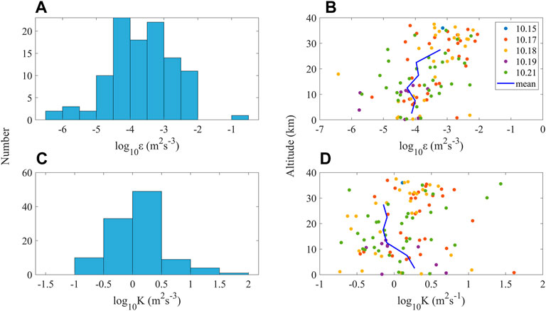
FIGURE 5. (A) Frequency distribution of the turbulent kinetic energy dissipation rate, (B) vertical distribution of the turbulent kinetic energy dissipation rate, (C) frequency distribution of the turbulent diffusion coefficient, and (D) vertical distribution of the turbulent diffusion coefficient. The blue lines in panels (C) and (D) denote the average values of ε and K in the vertical direction.

Figures 5A,C shows the frequency distribution histograms of all turbulent kinetic energy dissipation rates ε and turbulent diffusion coefficients K, while the vertical distributions of ε and K from October 15 to 21, 2021, are shown in Figures 5B,D. The values measured above 30 km and bellow 2 km are not considered herein because of the large noise present at these altitudes. The blue curves in Figures 5B,D represent the average values of ε and K in the vertical direction per 5 km; these values are used to observe the distributions more intuitively. Due to the considerable spatial variabilities in ε and K, a logarithmic mean is applied to these series to avoid distortion of the arithmetic averages caused by the magnitude differences. As shown in Figure 5A, the logarithmic mean value of ε varied from ${10}^{-7}$ to ${10}^{-2}$ $m^2{s}^{-3}$ and is mainly concentrated between ${10}^{-5}$ and ${10}^{-2}$ $m^2{s}^{-3}$, accounting for 89.8% of the total values. The maximum $lo{g}_{10}\epsilon$ is -2.29 $m^2{s}^{-3}$ observed at an altitude of 13.71 km on 21 October 2021. The ε term is more influenced by the Brunt-Vaisala frequency that by other factors due to the high power of this frequency in the calculation formula. Therefore, Figure 5B shows that although a relatively large $L_T$ value existed in the troposphere, the ε value is relatively small at that altitude due to the low $N^2$ value. Similarly, ε is generally large in the stratosphere. As shown in Figure 5C, the logarithmic mean value of K varies from ${10}^{-1.5}$ to ${10}^2$ $m^2{s}^{-1}$, and most of the K values are concentrated in the regions from ${10}^{-0.5}$ to ${10}^{0.5}$ $m^2{s}^{-1}$, accounting for 80% of the total values. The maximum $lo{g}_{10}K$ value is 1.06 $m^2{s}^{-1}$, identified at an altitude of 21.12 km on 17 October 2021.

In the free atmosphere, wind shear, heat convection, associated shear instabilities and convective instability, and gravity wave breaking drive turbulence at different scales ranging from several millimeters to kilometers; these processes thus play a potentially important role in the exchange of rare gases such as ozone and greenhouse gases between the troposphere and stratosphere. In this study, we obtained the newest available ozone partial pressure data recorded from October 10 to 21, 2021, and identified some disturbances in the vertical profile from these data. Combining the ozone partial pressure and turbulence information, the distributions of these two factors are shown in Figure 6, thus allowing us to observe the relationship between the exchange of ozone in the atmosphere and turbulence.

FIGURE 6

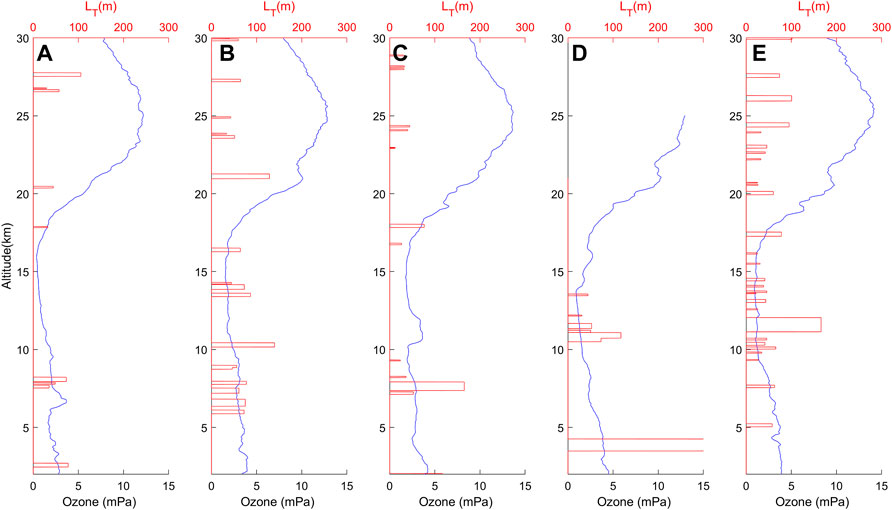
FIGURE 6. Distributions of the ozone partial pressure and Thorpe scale: panels (A)–(E) represent the data collected from October 15 to 21, 2021.

Figures 6A–E shows the distributions of the ozone partial pressure and turbulence from October 15 to 21, 2021. Some disturbances can be identified on the profiles near regions of turbulence. In Figure 6A, a slight increasing trend can be observed in the monotonically decreasing oxygen partial pressure profile near the turbulence at 8 km on October 15. Violent disturbances can also be identified near 26.5 km on the same day. As shown in Figure 6B, at altitudes of 5-10 km, where turbulences occur frequently on October 17, the partial pressure of oxygen is greatly disturbed. In the vicinity of the turbulence observed at approximately 21 km, violent ozone disturbances also occur. On the vertical profile obtained on October 18, an increase in ozone could be observed among the decreasing trend at approximately 8 km. Similar to Figures 6A–C), at heights of approximately 4 km in Figure 6D and of approximately 10-15 km in Figure 6E, the ozone vertical profiles exhibit some disturbances, and these disturbances are located near areas of turbulence. As seen from the figure, in most regions located near turbulence, ozone partial pressure perturbations occurred, thus proving that the generation of turbulence has a certain effect on the exchange of ozone concentration in the atmosphere. However, not all disturbances are caused by turbulence, and in many regions where turbulence does not occur, plenty of disturbances can still be observed.

To display the ozone distribution near a typical turbulence region more intuitively and observe the degree of perturbation, the ozone partial pressure gradient ((${\text{δ}}_{\text{ozone}}=\frac{\text{Ozone}\left(\text{k}\right)-\text{Ozone}\left(\text{k}-1\right)}{\text{z}\left(\text{k}\right)-\text{z}\left(\text{k}-1\right)}$) is calculated, as shown in Figure 7, where ∆z is 300 m. When the ozone partial pressure increases with altitude, ${\delta }_{ozone}$ is positive, and vice versa. If an ozone perturbation occurs, the distribution of the ozone gradient suddenly varies in the vertical direction. Figures 7A–E mainly show 5 ${\delta }_{ozone}$ values calculated above and below 750 m near the 5 regions of largest turbulence from October 15 to 21 October 2021.

FIGURE 7

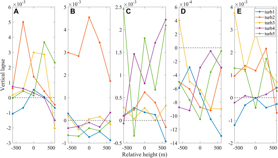
FIGURE 7. Distributions of the ozone gradient above and below 750 m near the 5 regions of largest turbulence: panels (A–E) represent the data collected from October 15 to 21, 2021.

Figure 7A shows that on the day of 15 October 2021, ${\delta }_{ozone}$ suddenly changed with increasing altitude near the 5 layers of greatest turbulent, indicating the generation of ozone perturbations. As shown in Figure 7A, the ${\delta }_{ozone}$ near the first, second, third and fifth turbulence regions would have been suddenly increasing with the altitude. The ozone profiles monotonically increased below the fourth turbulence regions and decreased suddenly due to the occurrence of turbulence. From Figure 7B, we can see that the distribution curve bumped up near the second and fourth turbulence regions; near the first and third turbulence region, the curve decreases rapidly and returns from positive to negative. No obvious disturbance is identified in the vicinity of the fifth turbulence region, and the same phenomenon is observed on other days, such as in the vicinity of the third turbulence region on October 18. All these results indicate that not all turbulence causes changes in the ozone vertical decline rate. The distributions of ${\delta }_{ozone}$ shown in Figures 7C–E are similar to those displayed in the first two figure panels. Most turbulence causes the ${\delta }_{ozone}$ distribution curve to generate a sudden turn. It can also be seen that near the fourth and fifth turbulence on October 18, multiple disturbances occur with the increase of altitude, which indicates that there are also other factors influencing the ozone perturbation.

Figure 6 shows that most disturbances were not generated near regions of turbulence. Pan et al. (2010) pointed out that the development and breaking of gravity waves can produce ozone exchanges (Pan et al., 2010), and gravity waves can also affect stratospheric ozone through chemical reactions associated with polar stratospheric cloud particles (Carslaw et al., 1998; Spang et al., 2018). Therefore, to determine the atmospheric conditions suitable for ozone disturbance generation, the change rates of the ozone gradient ${\text{δ}}_{\text{ozone}}^2=\frac{{\text{δ}}_{\text{ozone}}\left(\text{k}\right)-{\text{δ}}_{\text{ozone}}\left(\text{k}-1\right)}{\text{z}\left(\text{k}\right)-\text{z}\left(\text{k}-1\right)}$ in the vertical direction were calculated herein, as shown with the $N^2$ and shear conditions in Figure 8 and Figure 9. The declining rate of ozone represents the vertical-direction gradient; the faster the gradient changes, the stronger the ozone disturbance was, and the greater the absolute value of ${\delta }_{ozone}^2$ was.

FIGURE 8

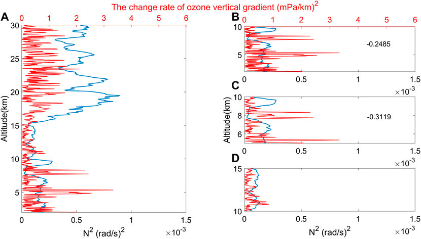
FIGURE 8. Distributions of $N^2$ (blue line) and the change rates of the ozone gradient (red line) at different altitudes on 15 October 2021: (A) 2–30 km, (B) 2–10 km, (C) 5–10 km and (D) 10–15 km.

FIGURE 9

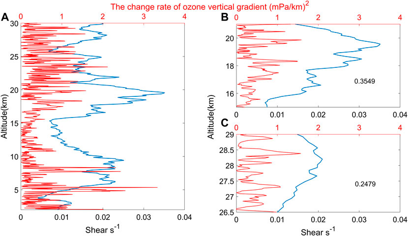
FIGURE 9. Distributions of the wind shear (blue line) and ozone gradient change rate gradient (red line) at different altitudes on 15 October 2021: (A) 2–30 km, (B) 15–21 km, and (C) 26.5–29 km.

The $N^2$ and ozone perturbation distributions identified at different altitudes are shown in Figure 8. Figure 8A shows the vertical profile of $N^2$ and the change rate of the ozone gradient from the 2 to 30 km on 15 October 2021; the smaller $N^2$ value is, the greater the static instability of the atmosphere is. In the low and middle troposphere, where $N^2$ is high, the change rate of the ozone gradient is relatively small; the specific relationship between these factors is shown in Figure 8B. As shown in Figures 8B, 2 obvious ozone perturbations are identified at altitudes of approximately 5 km and 8 km. The $N^2$ values at these altitudes are both at low levels. The corresponding region is selected, as shown in Figure 8C. The cubic spline method is used to fit the two factor profiles and calculate the correlation coefficients. At altitudes ranging from the 2 to 10 km, the correlation coefficient between $N^2$ and the change rate of the ozone gradient is -0.2785, while at 5-10 km, this value is -0.3119. Figure 8D shows the relationship between $N^2$ and ozone perturbations in the upper troposphere. It should be noted that at altitudes of 10-15 km, the $N^2$ values are generally small, but the disturbances are not strong. By combining the $N^2$ values obtained in the three regions mentioned above, we preliminarily concluded that ozone disturbances are more likely to occur when the static instability of the atmosphere changes suddenly with altitude. In the stratosphere, with increasing ozone concentrations, the change rates are generally large, but a series of disturbances, such as those identified at altitudes of 20.5, 23.4 and 29.2 km, are also found. All of these disturbances are located in regions where the $N^2$ values are relatively small compared to the surrounding regions. The conclusion is the same as that obtained above. However, at altitudes of 18.3, 19.8 and 28.37 km, large ozone disturbances are observed corresponding to small $N^2$ values. As shown in Figure 9, which displays the wind shear and ozone perturbation distributions at different altitudes, the 3 sets of disturbances all occur at altitudes where the wind shear was high. This finding indicates that shear instability is another important factor promoting the development of ozone disturbances in the stratosphere. We know that large wind shears are an important source of waves (Fritts et al., 2006; Pramitha et al., 2015) and are crucial for Kelvin-Helmholtz billows (Lane et al., 2012). The stratosphere-troposphere exchange (STE) caused by the breaking of gravity waves can also influence the distribution of ozone.

Figure 9A shows the wind shear and ozone perturbation distributions from the 2 to 30 km. In the troposphere, the change rates of the ozone gradient are not at high levels near the wind shear maxima. Therefore, shear instability is not the main factor affecting the observed tropospheric ozone disturbances but mainly plays a role in the stratosphere. As shown in Figure 9B, at 15-21 km, a positive correlation is found be-tween the wind shear and ozone disturbance, with a correlation coefficient of 0.3549. In Figure 9C, a large ozone perturbation can be seen at a height of approximately 28.3 km, where the shear instability is relatively strong. Combining this finding with Figure 8 and Figure 9, this ozone perturbation is found to have been influenced mostly by static instability in the troposphere and by both static instability and shear instability in the stratosphere.

The change rate of the ozone vertical gradient from October 17 to 21, 2021, is calculated and is shown in Figure 10 to verify the above conclusions. Figures 10A–D show the ozone perturbation distribution, and the $N^2$ values shown in Figures 10E–H reflect the wind shear and ozone perturbation conditions.

FIGURE 10

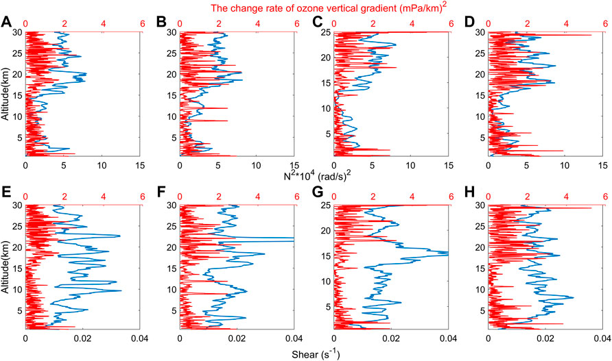
FIGURE 10. Panels (A)–(D) show the distributions of the $N^2$ values (blue line) and ozone gradient change rates (red line) from October 17 to 21, 2021; panels (E)–(H) show the distributions of the wind shear (blue line) and ozone gradient change rates (red line) from October 17 to 21, 2021.

Figures 10A–D shows that in the troposphere, the $N^2$ value is relatively small compared to the surrounding regions at the altitudes corresponding to large ozone perturbations, such as the low-troposphere layer from October 17 to 19, the 11 and 12.5 km heights on October 17, the 2.5 and 9 km heights on October 18, the 1.5 km height on October 19 and the 10 km height on October 21. In the stratosphere, static instability and shear instability work alone or mutually to influence the emergence of ozone perturbations. In Figures 10A–E, on 17 October 2021, at altitudes ranging from 25 to 26 km, a large ozone perturbation can be observed; correspondingly, the $N^2$ values all suddenly decrease. At heights of approximately 26 and 29.5 km, the large observed wind shears are conducive to the emergence of large perturbations. The same conclusions can be obtained on other days. In the stratosphere, from October 18 to 21, 2021, most ozone disturbances occurred at altitudes at which the $N^2$ value is relatively small or the wind shear is relatively large, such as at 19 and 25 km in Figures 10B–F, 18 and 21 km in Figures 10C–G, and 20 km in Figures 10D–H. Some disturbances not corresponding to the positions of the relatively-low $N^2$ values or relatively-high wind shear can also be seen in Figure 10. Wei et al. (2016) and Chang et al. (2021) have confirmed that the eddy ozone flux is also crucial for the ozone distribution (Weiet al., 2016; Chang et al., 2021). The search for other factors affecting ozone perturbations will thus be a major part of subsequent research.

Conclusion and discussion

Sounding data collected from October 17 to 21, 2021, over east China were used in this study to analyze the connection between turbulence and ozone perturbations. The specific analyzed parameters included the Thorpe scale, turbulent kinetic energy dissipation rate, turbulent diffusion coefficient, ozone vertical gradient and ozone vertical gradient change rate. After analyzing the distribution characteristics of these parameters and the atmospheric environment, we obtained some main conclusions, as described below.

The regions in which turbulence activity is relatively frequent throughout the study period included the 5–10 km and 10–15 km height ranges corresponding to the middle and upper troposphere. The turbulence number densities at these heights were 3.2 and 3.5, respectively. The strong turbulent layer observed in the middle troposphere is mainly caused by dynamic instability in which the wind shear is relatively large and the Ri value is mainly between 0 and 0.25. At 10-15 km, the $N^2$ value is at a low level, and Ri is less than zero at some heights. The atmospheric static instability is strong at this altitude, facilitating the generation of turbulence. In the low-troposphere layer, thermal convection and shear instability work together, which is beneficial for the emergence of large-scale turbulence. The largest $L_T$ value obtained at this altitude is 394 m; this value is much higher than those obtained for other layers. In addition, the turbulence observed near the tropopause and lower stratosphere could thus be attributed to the enhanced dynamic instability and breaking of Kelvin-Helmholtz waves (Browning et al., 1973). The turbulent kinetic energy dissipation rate and diffusion coefficient are calculated as $N^2$ and $L_T$, and the former is more sensitive to the stratification stability of the atmosphere than the latter. These values are generally small in the troposphere and large in the stratosphere. However, because of the existence of relatively strong turbulence in the low and middle troposphere, both ε and K exhibit high levels at these altitudes.

Turbulence plays an important role in the vertical mixing of air in the atmosphere (Sunilkumar et al., 2015), which in turn governs the vertical distribution of trace gases and the exchange of air particulates (Ko and Chun 2022). As an important trace gas, ozone plays an important role in global climate change. Therefore, it is particularly important to understand the distribution of ozone disturbances and their influencing factors (Zhang et al., 2018; He et al., 2020b; Liu and Hu 2021). In this study, the five largest-scale turbulences recorded throughout the study period were selected from the daily data, and the vertical ozone partial pressure decline rate changed dramatically around most of these events. The change rate of the ozone vertical gradient is severely influenced by atmospheric instability. In the troposphere, ozone perturbations occur most frequently in regions where atmospheric static instability is relatively strong; in the stratosphere, shear instability is also an important factor promoting the development of ozone disturbances. Thermal convection and large wind shears work alone or mutually to induce the emergence of ozone perturbations.

In this study, we used only a group of individual cases to analyze the primary influencing factors associated with ozone disturbances, such as turbulence, the Brunt-Vaisala frequency and wind shear. However, it can be seen from the results de-scribed above that not all ozone disturbances are related to these factors. Exploring the other factors that influence the vertical distribution of ozone is a topic we plan to study in the future.

Data availability statement

The original contributions presented in the study are included in the article/supplementary materials, further inquiries can be directed to the corresponding author.

Author contributions

ZQ and YH designed the experiments; ZQ, XZ and YF performed the experiments; ZQ and XY analysed the data; ZQ wrote the paper. All authors have read and agreed to the published version of the manuscript.

Funding

This research was funded by the National Natural Science Foundation of China (Grant no. 41875045) and by the Hunan Outstanding Youth Fund Project (Grant no. 2021JJ10048).

Acknowledgments

This study was supported by the National Natural Science Foundation of China (Grant no. 41875045), the Hunan Outstanding Youth Fund Project (Grant no. 2021JJ10048) and the “Western Light’’ Cross-Team Key Laboratory Cooperative Research Project of the Chinese Academy of Sciences.

Conflict of interest

The authors declare that the research was conducted in the absence of any commercial or financial relationships that could be construed as a potential conflict of interest.

Publisher’s note

All claims expressed in this article are solely those of the authors and do not necessarily represent those of their affiliated organizations, or those of the publisher, the editors and the reviewers. Any product that may be evaluated in this article, or claim that may be made by its manufacturer, is not guaranteed or endorsed by the publisher.

References

Browning, K. A., Bryant, G. W., Starr, J. R., and Axfordti, D. N. (1973). Air motion within kelvin-helmholtz billows determined from simultaneous Doppler radar and aircraft measurements.

Google Scholar

Carslaw, K., Wirth, M., Tsias, A., Luo, B., Dörnbrack, A., Leutbecher, M., et al. (1998). Increased stratospheric ozone depletion due to mountain-induced atmospheric waves. Nature 391, 675–678. doi:10.1038/35589

CrossRef Full Text | Google Scholar

Chan, L. Y., Chan, C. Y., Liu, H. Y., Christopher, S., Oltmans, S. J., and Harris, J. M. (2000). A case study on the biomass burning in southeast asia and enhancement of tropospheric ozone over Hong Kong. Geophys. Res. Lett. 27 (10), 1479–1482. doi:10.1029/1999GL010855

CrossRef Full Text | Google Scholar

Chang, S., Shi, C., Guo, D., and Xu, J. (2021). Attribution of the principal components of the summertime ozone valley in the upper troposphere and lower stratosphere. Front. Earth Sci. (Lausanne). 8. doi:10.3389/feart.2020.605703

CrossRef Full Text | Google Scholar

Chang, S., Zheng, S., Zhu, Y., Shi, W., and Luo, Z. (2020). Response of ozone to a gravity wave process in the UTLS region over the Tibetan plateau. Front. Earth Sci. (Lausanne). 8. doi:10.3389/feart.2020.00289

CrossRef Full Text | Google Scholar

Cho, J. Y. N., Reginald, E. N., Anderson, B. E., Barrick, J. D. W., and Lee Thornhill, K. (2003). Characterizations of tropospheric turbulence and stability layers from aircraft observations. J. Geophys. Res. 108 (20), 8784. doi:10.1029/2002JD002820

CrossRef Full Text | Google Scholar

Clayson, C. A., and Kantha, L. (2008). On turbulence and mixing in the free atmosphere inferred from high-resolution soundings. J. Atmos. Ocean. Technol. 25 (6), 833–852. doi:10.1175/2007JTECHA992.1

CrossRef Full Text | Google Scholar

Cohn, S. A. (1995). Radar measurements of turbulent eddy dissipation rate in the troposphere: a comparison of techniques. J. Atmos. Ocean. Technol. 12, 85–95. doi:10.1175/1520-0426(1995)012<0085:rmoted>2.0.co;2

CrossRef Full Text | Google Scholar

Crawford, W. R. (1986). A comparison of length scales and decay times of turbulence in stably stratified flows. J. Phys. Oceanogr. 1611, 1847–1854. doi:10.1175/1520-0485(1986)016<1847:acolsa>2.0.co;2

CrossRef Full Text | Google Scholar

Dehghan, A., Hocking, W. K., and Srinivasan, R. (2014). Comparisons between multiple in-situ aircraft turbulence measurements and radar in the troposphere. J. Atmos. Solar-Terrestrial Phys. 118, 64–77. doi:10.1016/j.jastp.2013.10.009

CrossRef Full Text | Google Scholar

Fritts, D. C., and Joan Alexander, M. (2003). Gravity wave dynamics and effects in the middle atmosphere. Rev. Geophys. 41 (1). doi:10.1029/2001RG000106

CrossRef Full Text | Google Scholar

Fritts, D. C., Vadas, S. L., Wan, K., and Werne, J. A. (2006). Mean and variable forcing of the middle atmosphere by gravity waves. J. Atmos. Solar-Terrestrial Phys. 68 (3–5), 247–265. doi:10.1016/j.jastp.2005.04.010

CrossRef Full Text | Google Scholar

Fritts, D. C., Wan, K., Franke, P. M., and Tom, L. (2012). Computation of clear-air radar backscatter from numerical simulations of turbulence: 3. Off-zenith measurements and biases throughout the lifecycle of a kelvin-helmholtz instability. J. Geophys. Res. 117 (17). doi:10.1029/2011JD017179

CrossRef Full Text | Google Scholar

Fukao, S., Yamanaka, M. D., Ao, N., Hocking, W. K., Sato, T., Yamamoto, M., et al. (1994). Seasonal variability of vertical eddy diffusivity in the middle atmosphere 1. Three-year observations by the middle and upper atmosphere radar. J. Geophys. Res. Atmos. 99, 18973–18987. doi:10.1029/94JD00911

CrossRef Full Text | Google Scholar

Gavrilov, N. M., Luce, H., Crochet, M., Dalaudier, F., and Fukao, S. (2005). Turbulence parameter Estimations from high-resolution Balloon temperature measurements of the MUTSI-2000 Campaign. Ann. Geophys, 23, 2401–2413. doi:10.5194/angeo-23-2401-2005

CrossRef Full Text | Google Scholar

He, Y., Zheng, S., and He, M. (2020a). The first observation of turbulence in northwestern China by a near-space high-resolution Balloon sensor. Sensors Switz. 20 (3), 677. doi:10.3390/s20030677

PubMed Abstract | CrossRef Full Text | Google Scholar

He, Y., Zheng, S., Zhou, L., He, M., and Zhou, S. (2020b). Statistical analysis of turbulence characteristics over the tropical western pacific based on radiosonde data. Atmosphere 11 (4), 386. doi:10.3390/ATMOS11040386

CrossRef Full Text | Google Scholar

He, Y., Zhu, X., Zheng, S., Zhang, J., Zhou, L., and He, M. (2021). Statistical characteristics of inertial gravity waves over a tropical station in the western pacific based on high-resolution GPS radiosonde soundings. JGR. Atmos. 126 (11). doi:10.1029/2021JD034719

CrossRef Full Text | Google Scholar

Hocking, W. K. (1988). Two years of continuous measurements of turbulence parameters in the upper mesosphere and lower thermosphere made with A 2-mhz radar. J. Geophys. Res. Atmos. 93, 2475–2491. doi:10.1029/JD093iD03p02475

CrossRef Full Text | Google Scholar

Jackman, C. H., Anne, R. D., Guthrie, P. D., and Stolarski, R. S. (1989). The sensitivity of total ozone and ozone perturbation scenarios in a two-dimensional model due to dynamical inputs. J. Geophys. Res. Atmos. 94. doi:10.1029/JD094iD07p09873

CrossRef Full Text | Google Scholar

Jiankai, Z., Tian, W., Xie, F., Sang, W., Guo, D., Chipperfield, M., et al. (2019). Zonally asymmetric trends of winter total column ozone in the northern middle latitudes. Clim. Dyn. 52 (7–8), 4483–4500. doi:10.1007/s00382-018-4393-y

CrossRef Full Text | Google Scholar

Kantha, L., and Hocking, W. (2011). Dissipation rates of turbulence kinetic energy in the free atmosphere: MST radar and radiosondes. J. Atmos. Solar-Terrestrial Phys. 73 (9), 1043–1051. doi:10.1016/j.jastp.2010.11.024

CrossRef Full Text | Google Scholar

Ko, H. C., and Chun, H. Y. (2022). Potential sources of atmospheric turbulence estimated using the Thorpe method and operational radiosonde data in the United States. Atmos. Res. 265, 105891. doi:10.1016/j.atmosres.2021.105891

CrossRef Full Text | Google Scholar

Lane, T. P., Sharman, R. D., Trier, S. B., Fovell, R. G., and Williams, J. K. (2012). Recent advances in the understanding of near-cloud turbulence. Bull. Am. Meteorol. Soc. 93 (4), 499–515. doi:10.1175/BAMS-D-11-00062.1

CrossRef Full Text | Google Scholar

Liu, M., and Hu, D. (2021). Different relationships between arctic oscillation and ozone in the stratosphere over the arctic in january and february. Atmosphere 12 (2), 129. doi:10.3390/atmos12020129

CrossRef Full Text | Google Scholar

Lobken, F. J. (1992). On the extraction of turbulent parameters from atmospheric density fluctuations. J. Geophys. Res. Atmos. 97, 20385–20395. doi:10.1029/92JD01916

CrossRef Full Text | Google Scholar

Maleska, S., Smith, K. L., and Virgin, J. (2020). Impacts of stratospheric ozone extremes on arctic high cloud. J. Clim. 33 (20), 8869–8884. doi:10.1175/JCLI-D-19-0867.1

CrossRef Full Text | Google Scholar

Miyazaki, K., Watanabe, S., Kawatani, Y., Tomikawa, Y., Takahashi, M., and Sato, K. (2010). Transport and mixing in the extratropical tropopause region in a high-vertical-resolution GCM. Part I: Potential vorticity and heat budget analysis. J. Atmos. Sci. 67 (5), 1293–1314. doi:10.1175/2009JAS3221.1

CrossRef Full Text | Google Scholar

Nastrom, G. D., and Eaton, F. D. (1997). Turbulence eddy dissipation rates from radar observations at 5-20 Km at white sands missile range, New Mexico. J. Geophys. Res. 102 (16), 19495–19505. doi:10.1029/97jd01262

CrossRef Full Text | Google Scholar

Pan, L. L., Bowman, K. P., Elliot, A., Wofsy, S. C., Zhang, F., James, F. B., et al. (2010). The stratosphere-troposphere analyses of regional transport 2008 experiment. Bull. Am. Meteorol. Soc. 91 (3), 327–342. doi:10.1175/2009BAMS2865.1

CrossRef Full Text | Google Scholar

Pierazzo, E., Garcia, R. R., Kinnison, D. E., Marsh, D. R., Lee-Taylor, J., and Crutzen, P. J. (2010). Ozone perturbation from medium-size asteroid impacts in the ocean. Earth Planet. Sci. Lett. 299 (3–4), 263–272. doi:10.1016/j.epsl.2010.08.036

CrossRef Full Text | Google Scholar

Pramitha, M., Venkat Ratnam, M., Taori, A., Krishna Murthy, B. V., Pallamraju, D., and VijayaRao, S. B. (2015). Evidence for tropospheric wind shear excitation of high-phase-speed gravity waves reaching the mesosphere using the ray-tracing technique. Atmos. Chem. Phys. 15 (5), 2709–2721. doi:10.5194/acp-15-2709-2015

CrossRef Full Text | Google Scholar

Qin, Z., Zheng, S., Yang, H., and Feng, Y. (2022). Case analysis of turbulence from high-resolution sounding data in northwest China. Front. Environ. Sci. 10. doi:10.3389/fenvs.2022.839685

CrossRef Full Text | Google Scholar

Ramaswamy, V., Chanin, M. L., Angell, J., Barnett, J., Gaffen, D., Gelman, M., et al. (2001). Stratospheric temperature trends: Observations and model simulations. Rev. Geophys. 39 (1), 71–122. doi:10.1029/1999RG000065

CrossRef Full Text | Google Scholar

Riley, J. J., and Erik, L. (2008). Stratified turbulence: A possible interpretation of some geophysical turbulence measurements. J. Atmos. Sci. 65 (7), 2416–2424. doi:10.1175/2007JAS2455.1

CrossRef Full Text | Google Scholar

Sharman, R. D., Trier, S. B., Lane, T. P., and Doyle, J. D. (2012). Sources and dynamics of turbulence in the upper troposphere and lower stratosphere: A review. Geophys. Res. Lett. 39 (12). doi:10.1029/2012GL051996

CrossRef Full Text | Google Scholar

Singh, N., JoshiChun, R. R. H., Pant, G. B., Damle, S. H., and Vashishtha, R. D. (2008). Seasonal, annual and inter-annual features of turbulence parameters over the tropical station pune (18 • 32 N, 73 • 51 E) observed with UHF wind profiler. Ann. Geophys. 26. doi:10.5194/angeo-26-3677-2008

CrossRef Full Text | Google Scholar

Spang, R., Hoffmann, L., Müller, R., Jens, U. G., Tritscher, I., Höpfner, M., et al. (2018). A climatology of polar stratospheric cloud composition between 2002 and 2012 based on MIPAS/envisat observations. Atmos. Chem. Phys. 18 (7), 5089–5113. doi:10.5194/acp-18-5089-2018

CrossRef Full Text | Google Scholar

Sunilkumar, S. V., Muhsin, M., Parameswaran, K., Venkat Ratnam, M., Ramkumar, G., Rajeev, K., et al. (2015). Characteristics of turbulence in the troposphere and lower stratosphere over the Indian peninsula. J. Atmos. Solar-Terrestrial Phys. 133, 36–53. doi:10.1016/j.jastp.2015.07.015

CrossRef Full Text | Google Scholar

Thorpe, S. A. (1977). Turbulence and mixing in a Scottish loch. Philos. Trans. Roy. Soc. Lond. 286A, 125–181.

Google Scholar

Wang, W. (2004). Heterogeneous structure of vertical distribution of atmospheric ozone (in Chinese). J. Yunnan Univ. 26 (2), 144–149.

Google Scholar

Wang, W., Matthes, K., Tian, W., Park, W., Shangguan, M., and Ding, A. (2019). Solar impacts on decadal variability of tropopause temperature and lower stratospheric (LS) water vapour: A mechanism through ocean–atmosphere coupling. Clim. Dyn. 52 (9–10), 5585–5604. doi:10.1007/s00382-018-4464-0

CrossRef Full Text | Google Scholar

Wang, Y., Wang, H., and Wang, W. (2020). A stratospheric intrusion-influenced ozone pollution episode associated with an intense horizontal-trough event. Atmosphere 11 (2), 164. doi:10.3390/atmos11020164

CrossRef Full Text | Google Scholar

Wei, D., Tian, W. S., and Chen, Z. Y. (2016). Upward transport of air mass during a generation of orographic waves in the UTLS over the Tibetan plateau. doi:10.6038/cjg20160303

CrossRef Full Text | Google Scholar

Wilson, R., Hubert, L., Dalaudier, F., and Lefrère, J. (2010). Turbulence patch identification in potential density or temperature profiles. J. Atmos. Ocean. Technol. 27 (6), 977–993. doi:10.1175/2010JTECHA1357.1

CrossRef Full Text | Google Scholar

Wilson, R., Dalaudier, F., and Luce, H. (2011). Can one detect small-scale turbulence from standard meteorological radiosondes? Atmos. Meas. Tech. 4 (5), 795–804. doi:10.5194/amt-4-795-2011

CrossRef Full Text | Google Scholar

Wilson, R., Luce, H., Hashiguchi, H., Shiotani, M., and Dalaudier, F. (2013). On the effect of moisture on the detection of tropospheric turbulence from in situ measurements. Atmos. Meas. Tech. 6 (3), 697–702. doi:10.5194/amt-6-697-2013

CrossRef Full Text | Google Scholar

Xia, Y., Huang, Y., and Hu, Y. (2018). On the climate impacts of upper tropospheric and lower stratospheric ozone. J. Geophys. Res. Atmos. 123 (2), 730–739. doi:10.1002/2017JD027398

CrossRef Full Text | Google Scholar

Xie, F., Li, J., Tian, W., Zhang, J., and Shu, J. (2014). The impacts of two types of El Niño on global ozone variations in the last three decades. Adv. Atmos. Sci. 31 (5), 1113–1126. doi:10.1007/s00376-013-3166-0

CrossRef Full Text | Google Scholar

Xu, X., Wang, Y., Xue, M., and Zhu, K. (2017). Impacts of horizontal propagation of orographic gravity waves on the wave drag in the stratosphere and lower mesosphere. J. Geophys. Res. Atmos. 122 (2111), 11,301–11,312. doi:10.1002/2017JD027528

CrossRef Full Text | Google Scholar

Yang, Y., Li, J., Wu, L., Yu, K., Du, Y., Sun, C., et al. (2017). Decadal Indian ocean dipolar variability and its relationship with the tropical pacific. Adv. Atmos. Sci. 34, 1282–1289. doi:10.1007/s00376-017-7009-2

CrossRef Full Text | Google Scholar

Zhang, J., Chen, H., Li, Z., Fan, X., Liang, P., Yu, Y., et al. (2010). Analysis of cloud layer structure in shouxian, China using RS92 radiosonde aided by 95 GHz cloud radar. J. Geophys. Res. 115 (23), D00K30. doi:10.1029/2010JD014030

CrossRef Full Text | Google Scholar

Zhang, J., Tian, W., Pyle, J. A., James, K., Abraham, N. L., Chipperfield, M. P., et al. (2022). Responses of arctic sea ice to stratospheric ozone depletion. Sci. Bull. 67, 1182–1190. doi:10.1016/j.scib.2022.03.015

CrossRef Full Text | Google Scholar

Zhang, J., Tian, W., Xie, F., Chipperfield, M. P., Feng, W., Son, S. W., et al. (2018). Stratospheric ozone loss over the eurasian continent induced by the polar vortex shift. Nat. Commun. 9 (1), 206. doi:10.1038/s41467-017-02565-2

PubMed Abstract | CrossRef Full Text | Google Scholar

Zhang, J., Tian, W., Xie, F., et al. (2019). Zonally asymmetric trends of winter total column ozone in the northern middle latitudes. Clim. Dyn. 52, 4483–4500. doi:10.1007/s00382-018-4393-y

CrossRef Full Text | Google Scholar

Zhang, J., Tian, W., Xie, F., Li, Y., Wang, F., Huang, J., et al. (2015). Influence of the El Niño southern oscillation on the total ozone column and clear-sky ultraviolet radiation over China. Atmos. Environ. 120, 205–216. doi:10.1016/j.atmosenv.2015.08.080

CrossRef Full Text | Google Scholar

Zhang, J., Zhang, S. D., Huang, C. M., Huang, K. M., Gong, Y., Gan, Q., et al. (2019). Latitudinal and topographical variabilities of free atmospheric turbulence from high-resolution radiosonde data sets. J. Geophys. Res. Atmos. 124 (8), 4283–4298. doi:10.1029/2018JD029982

CrossRef Full Text | Google Scholar

Zhang, S. D., Fan, Y., Huang, C. M., and Huang, K. M. (2012). High vertical resolution analyses of gravity waves and turbulence at a midlatitude station. J. Geophys. Res. 117 (2). doi:10.1029/2011JD016587

CrossRef Full Text | Google Scholar

Zhao, X. R., Sheng, Z., Li, J. W., Yu, H., and Wei, K. J. (2019). Determination of the ‘wave turbopause’ using a numerical differentiation method. J. Geophys. Res. Atmos. 124 (20), 10592–10607. doi:10.1029/2019JD030754

CrossRef Full Text | Google Scholar