Glyphosate and AMPA have low mobility through different soil profiles of the prosecco wine production area: A monitoring study in north-eastern Italy

Contamination of the environment by glyphosate (GLP) and its metabolite aminomethylphosphonic acid (AMPA) is still of major concern worldwide due to specific interactions among these molecules and soil and water. Two monitoring sites were established in the Prosecco wine production area (Conegliano and Valdobbiadene) in northeastern Italy, which has been included in UNESCO’s World Heritage List since 2019. The study aims to increase the knowledge about GLP dynamics in this area where it has been intensively used by farmers and the potential risk for groundwater pollution is still debated. Each site was equipped with two soil-water monitoring stations consisting of multisensor soil probes and suction cups at three soil depths (10, 30, and 70 cm). Soil and water were sampled for 10 and 6 months, respectively, and analyzed for GLP and AMPA concentrations, for a total of 242 samples to describe their vertical movement and dissipation dynamics. Soil properties, in particular, the different forms of Fe and Al oxide contents, and Freundlich adsorption coefficients were quantified along the soil profile. First attempts showed that glyphosate dissipation time was 36 ± 8 days in Conegliano and Valdobbiadene soils and fully completed in both after 6 months. In contrast, AMPA dissipation dynamic —first described by an original equation—was longer than that of GLP and fully dissipated after almost 300 days. GLP showed a strong binding affinity with clay and Fe and Al chelated to soil organic matter, which likely acted as cation bridges and in turn led to low GLP mobility. GLP and AMPA were mostly detected after heavy rainfall events at 70 cm depth, likely bypassing the porous matrix of the intermediate layers.

Introduction

Glyphosate (GLP) is one of the most-used broad-spectrum, systemic, and postemergence herbicides worldwide, with sales estimates of about 825,804 tons in 2014—of which 90% was used by the agricultural sector (Antier et al., 2020)—and expected 6.5% annual sales growth between 2016 and 2024 (Ahuja and Raeat, 2017). In agricultural lands, GLP-based agrochemicals are sprayed mainly before planting the crop or postharvest during the intercropping period to control weeds’ growth. Glyphosate may also be used in preharvest on cereal, oilseed, and pulse crops to aid harvesting and protect grain quality. Crops treated annually with GLP are annual (e.g., cereals and oilseeds) and perennial crops, like orchards and vineyards (Antier et al., 2020).

GLP is usually considered to have reduced mobility in soil due to its high affinity with clay minerals, soil oxides, and hydroxides (Vereecken, 2005). As a polyprotic acid, its charge depends on soil pH resulting in complex sorption equilibrium dynamics. GLP commonly occurs as an anion, and for this reason it can only be sorbed onto variable-charge sites (e.g., Al and Fe oxides and 1:1 layer silicate clays in acidic soils). Moreover, its molecular structure makes interaction with soil organic matter (SOM) controversial compared to most nonpolar pesticides due to 1) dominating repulsive forces between negatively charged molecules—GLP and SOM components and 2) blocking effect of SOM on other sorption sites that can lead to low GLP adsorption (Ololade et al., 2014). Conversely, the SOM propensity to promote poorly ordered Al and Fe might increase the soil sorption capacity of GLP (Okada et al., 2016), although this has been little studied so far and deserves attention, especially because it is strongly influenced by site-specific conditions. Furthermore, the presence of phosphate in the soil might worsen the sorption capacity of the molecule by competing with bonding sites on Al-OH and Fe-OH surfaces (Borggaard and Gimsing, 2008). At the same time, GLP could be sorbed on phosphates through a metal cation bond (Al³⁺ and Fe³⁺, or Ca²⁺and Mg²⁺) as suggested by some authors (Morillo et al., 1997; Nowack and Stone, 2006). Glyphosate adsorption in the soil is usually described by a nonlinear Freundlich sorption isotherm, where the sorption coefficient (K_f) values can range from 0.6 to 700 (Vereecken, 2005; EFSA, 2015), depending on soil-specific characteristics. The main metabolite of GLP, aminomethylphosphonic acid (AMPA), is also characterized by high adsorption, depending on soil pH, Al and Fe oxide contents, and available phosphorus and carbonate content.

The low mobility of GLP and AMPA should exclude the potential risk of leaching to groundwater (Borggaard and Gimsing, 2008). However, large discrepancies exist in the literature about their transfer toward water. Indeed, GLP and AMPA are frequently detected not only in surface waters, e.g., transported in runoff or by erosion processes, but also in groundwater, increasing concerns about GLP use in agriculture as in urban areas or railways and raising questions on the driving factors that lead to contamination of the surface and belowground aquatic environment (Blake and Pallett, 2018). Furthermore, the high GLP and AMPA solubility in water (11.6 and 1466.5 g l⁻¹, respectively) (Pesticide Property DataBase by IUPAC, Lewis and Tzilivakis, 2017) increases the risk of being transported in the aqueous phase. Studies investigating GLP mobility reported that leaching may occur (Kjær et al., 2003; Stone and Wilson, 2006) under specific conditions, e.g., through macropore- or crack-mediated preferential flow pathways. The leachability of GLP could also be aggravated in soils that are phosphate-saturated or after phosphate addition to soil (De Jonge et al., 2001). Moreover, some studies emphasized that GLP could be released by root exudation when target plants start to decompose, bypassing the rootzone (Neumann et al., 2006; Laitinen et al., 2007; Viti et al., 2019).

The persistence of GLP in the soil environment is mainly influenced by the microbiota (Sprankle et al., 1975), as well as by different soil conditions—such as water content, temperature, and particle size distribution (Bento et al., 2016). It follows that site-specific conditions can strongly affect GLP persistence, the dissipation half-life in soils (DT₅₀) being of the order of 1.5–50 days (Bento et al., 2016; Okada et al., 2019) up to 8 months (Laitinen et al., 2006). The persistence, in addition to mobility and leaching, is particularly important for areas where GLP is broadly used, as recently reported by Gairhe et al. (2021). Its use in vineyards is one of the major concerns in the Prosecco wine production area in northeastern Italy, which has been included (since July 2019) in UNESCO’s World Heritage List. Here, GLP has been used for decades and its application is still debated, mainly by the local population and authorities due to sporadic GLP findings in groundwaters (De Polo et al., 2019). Therefore, in 2019, the Prosecco Conegliano–Valdobbiadene DOCG consortium decided to ban the use of GLP by encouraging alternative vineyard management, such as the use of mechanical mowing (Consorzio di Tutela DOCG Conegliano Valdobbiadene, 2019). However, scarce information is available on GLP and AMPA behavior in these soils. It is therefore imperative to understand how these molecules move, bind, and degrade in the Prosecco area to improve their utilization for weed control.

The aims of this study were therefore 1) to understand the site-specific GLP adsorption, dissipation, and propensity to leaching in two different agricultural soils and 2) to identify the driving factors leading to specific soil–water-contaminant interactions in the wine-growing terroir of the Prosecco wine production.

Materials and methods

Experimental site description and field setup

The study was conducted in two experimental sites located in Conegliano and Valdobbiadene municipalities (NE Italy, Figure 1), 35 km apart, which are included in a vast foothill and hilly agricultural area of extensive vineyard cultivations. The study area is part of the wine-growing terroir of the DOCG Prosecco wine, which includes 15 municipalities (about 18,000 ha). The experimental sites, already included in a wider network of monitored sites within a project on drinking groundwater quality monitoring and protection (Perri et al., 2012; Zovi et al., 2017), were selected due to their location near catchment wells used for drinking water purposes. It should be noted that no GLP-based herbicides were used in the two experimental sites at least 3 years prior to our study.

FIGURE 1

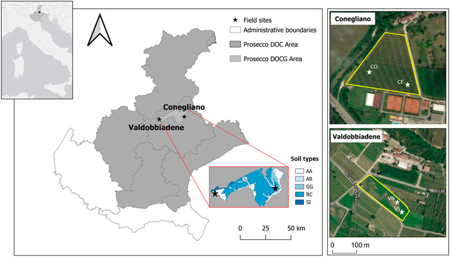
FIGURE 1. Location of the experimental area in the Veneto region and of the two monitored sites (black stars) within the Prosecco DOCG area, Conegliano and Valdobbiadene (satellite images on the right). Soil types within the DOCG area—and the corresponding geomorphological origin—are also reported (AA: ancient, gravelly, calcareous high plain; AR: recent high plains and terraces, gravelly and calcareous; GG: Pleistocene moraine amphitheaters consisting of long, arcuate hills; RC: pre-Alpine hilly reliefs placed at the foot of massifs; SI: long and articulated pre-Alpine mountain ridges, consisting of hard and marly limestone) (ARPAV, 2008). The white stars indicate the two monitoring stations identified in each site with the corresponding names.

The Conegliano site (45° 53.999′N, 12° 17.732′E) (Figure 1, 66 m a.s.l.) falls within a flat grassed vineyard, 1.8 ha in size, close to the Monticano river. The climate is subhumid, with a mean annual temperature of 14.2°C, ranging between a mean minimum of 1.2°C and a mean maximum of 29.5°C in January and July, respectively, and annual rainfall of 1200 mm distributed uniformly throughout the year (1994–2019 data time series; ARPAV, 2020). According to the regional soil map (scale 1:50,000), the soil of the area is homogeneous (Figure 1) and geomorphologically originated from recent gravelly and calcareous high plains and terraces (ARPAV, 2008). The soil is classified as a Fluvic Cambisol (WRB, 2014; ARPAV, 2019) with a silty loam texture, pH of 8.4, 1.01% of organic carbon, and cation exchange capacity (CEC) of 15.7 meq 100 g⁻¹ as average values through the soil profile (Table 1). The Conegliano site has two aquifer levels, the shallow one, consisting mainly of gravel in a silty or sandy matrix, fluctuates during the year between 1.5 and 6.3 m depth depending on the season, while the deep one develops below 10 m depth. The Valdobbiadene site (45° 53.148′N 11° 58.658′E) (Figure 1, 176 m a.s.l.) is a 0.7 ha flat meadow surrounded by vineyards, about 1 km north of the Piave river. The site has a similar climate to the Conegliano one, with a mean annual temperature of 13.2°C, registering a mean minimum temperature of 0.5°C in January and a mean maximum of 28.7°C in July, and annual rainfall of 1470 mm with November being the wettest month—195 mm (1994–2019 data time series; ARPAV, 2020). The soil of the Valdobbiadene area is homogeneous (Figure 1), gravelly, and calcareous. The soil of this area originates from ancient high plain soils consisting of locally terraced fluvioglacial deposits and secondarily alluvial plains of pre-Alpine streams (ARPAV, 2008). It is a thin Haplic Regosol (WRB, 2014; ARPAV, 2019), sandy loam, which quickly turns into a gravel layer roughly below 50 cm depth, delimiting the top boundary of the ancient Piave riverbed. The soil has a pH of 8.4, 0.86% of organic carbon, and CEC of 10.6 meq 100 g⁻¹ as average values through the soil profile (Table 1). The groundwater level fluctuates yearly between 4 and 8 m depth and is strongly affected by the Piave river water levels.

TABLE 1

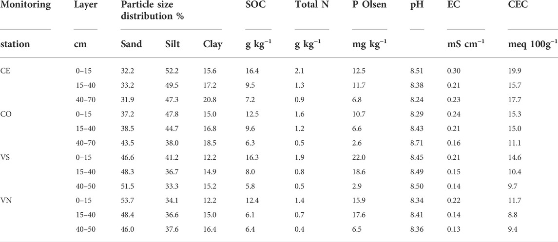
TABLE 1. Soil chemical properties at the four monitoring stations as a function of depth. SOC refers to soil organic carbon (g kg⁻¹), Total N is total nitrogen (g kg⁻¹), P Olsen is available phosphorus (mg kg⁻¹), EC is electrical conductivity (mS cm⁻¹), and CEC is cation exchange capacity (meq 100 g⁻¹).

Two soil-water monitoring stations of 25 m² size each were set up on each site during September 2018, hereafter referred to as CE and CO for Conegliano (inter-row grass vineyard) and VS and VN for Valdobbiadene (grassland) (Figure 1). Each experimental site was equipped with a weather station that recorded air temperature, relative humidity, solar irradiance, wind speed, and rainfall every 5 min (HD35EDLM.E, DeltaOhm, Padova, Italy). Multisensor probes—soil temperature (T, °C) and soil water content (SWC, m³ m⁻³) (HD3910.1, DeltaOhm, Padova, Italy)—and suction cups (SPE20 pore water sampler, METER Group AG München) were installed at 10, 30, and 70 cm depth in the four monitoring stations. The multisensor probes were set to collect data at hourly intervals. Prior to field installation, the soil moisture sensors, operating with frequency domain reflectometry technology, were calibrated in the laboratory to an accuracy of ±3%. The pore water samplers had a porous polyethylene-nylon cup whose interaction with GLP (i.e., adsorption), tested in the laboratory before field installation (Supplementary Figure 1S), was not significant. Due to the presence of the gravel bed below 50 cm depth in Valdobbiadene and the consequent poor functioning of the suction cups, two pan lysimeters were installed at 70 cm depth to collect the leachate.

Characterization of soil profiles

A hydraulic sampler was used to collect undisturbed soil cores in two random positions in each monitoring station down to 70 cm at Conegliano and 50 cm at Valdobbiadene before the experiment. A tractor-mounted double-cylinder core sampler (5 cm diameter) was used for sampling, to reduce soil compaction by slowly drilling soil layers with parallel cutting edges (Dal Ferro et al., 2020). Each soil core was measured to confirm it matched the full length of the hole (Grossman and Reinsch, 2002). After that, soil columns in each monitoring station were separated into distinct layers (0–15, 15–40 cm, and 40–70 in CE and CO; 0–15, 15–40 cm, and 40–50 cm in VS and VN), bulked, and later analyzed for their chemical and physical properties (Table 1). Soil texture was determined using a particle size analyzer (Mastersizer 2000, Malvern Panalytical Ltd., Spectris Company) according to Bittelli et al. (2019), soil organic carbon (SOC) and total nitrogen (Total N) content were determined by the flash combustion method with a CNS-analyzer (vario MACRO cube, Elementar Analysensysteme GmbH), pH and electrical conductivity (EC) were measured by an electrode in soil suspensions with a soil-to-water ratio of 1:2.5 (w/v), the cation exchange capacity (CEC) was measured using the BaCl₂-triethanolamine method, and the assimilable phosphate (P Olsen) was determined using the Olsen method.

Determination of Al and Fe oxides in soil

Mineralogical iron (Fe) and aluminum (Al) oxides were measured along the soil profiles at 0–15, 15–40, and 40–70 cm for Conegliano and 0–15, 15–40, and 40–50 cm for Valdobbiadene. Two methods were applied to determine 1) poorly ordered Al and Fe oxides (oxalate-extractable, hereafter labeled as Al_Ox and Fe_Ox, respectively ) and 2) soil organic matter-chelated Al and Fe (sodium pyrophosphate-extractable, hereafter labeled as Al_Som and Fe_Som , respectively).

Poorly ordered Al and Fe oxides, also called “amorphous”, were determined using the ammonium oxalate in darkness extraction method as reported by McKeague et al. (1971). The soils were air-dried and sieved at 0.1 mm. Due to the high calcium carbonate content, soil samples were pretreated with a solution of ammonium acetate (pH 5.5) prior to the extraction. For the extraction procedure, 0.5 g of pretreated air-dried soil was weighed in a polypropylene tube and spiked with 30 ml of an ammonium oxalate-oxalic acid solution at pH 3. The samples were shaken for 3 h in darkness and centrifuged. The solution was then separated from the soil and collected in a polyethylene tube. Soil organic matter-chelated metals were extracted using a solution of sodium pyrophosphate at pH 10. In this case, the alkaline environment is preferred since the extraction of crystalline and amorphous forms is slight (Bascomb, 1968). A volume of 40 ml solution was added to 0.4 g of air-dried, 0.1 mm sieved soil, and the samples were shaken for 16 h at 20°C. The samples were then centrifuged and filtered using mixed cellulose ester (MCE) membrane filters with a pore diameter of 0.45 µm. All of the solutions were analyzed by ICP-OES for the Al and Fe content, expressed as mg kg⁻¹.

Adsorption isotherms of glyphosate

A batch adsorption experiment was performed following the OECD guideline using the batch equilibrium method (OECD, 2000). The chemical standard of glyphosate acid (98.6% purity) was purchased from Dr. Ehrenstorfer (LGC Labor GmbH, Augsburg, Germany). Five different concentrations of GLP in the range of 0.1–25 μg g⁻¹ of dry soil were tested, with three replicates each. The adsorption study was performed for three different soil layers covering the whole soil profile (0–15, 15–40, and 40–70 cm for CE and CO and 0–15, 15–40, and 40–50 cm for VS and VN), with the exclusion of the gravel layer. Uncontaminated soils obtained from the initial sampling—lack of glyphosate in the soil was checked in the laboratory—were air-dried, sieved at 2 mm, and stored at room temperature before the experiment. First, 39 ml of 0.01 M CaCl₂ was added to 1 g of dry weight soil in 50-ml polypropylene tubes and shaken at 200 rpm for 24 h at 20°C. The soil slurry was then spiked with 1 ml of the corresponding GLP solution, with three replicates for each concentration. After shaking for 24 h, the tubes were centrifuged at 3,000 rpm for 20 min, and an aliquot of supernatant (∼1 ml) was taken and stored in a refrigerator at +4°C before the UHPLC-MS analysis. The amount of GLP adsorbed on the soil was calculated as the difference between the amount initially present in the solution and the amount remaining at the end of the experiment.

Adsorption data were fitted to the Freundlich adsorption isotherm model by nonlinear optimization:

$C_s=K_f{C}_w^{\left(\frac{1}{n}\right)}[1]$

where C_s (μg g⁻¹) is the amount of GLP adsorbed into the soil, C_w (μg ml⁻¹) is the concentration of GLP in the aqueous phase, K_f [μg^1–1/n (ml)^1/n g⁻¹] is the Freundlich adsorption coefficient, and 1/n is the regression constant or measure of nonlinearity. To compute the unknown empirical coefficient, the least square method was applied. Moreover, to compare K_f among sites and depths, the depth-averaged 1/n coefficient was calculated and used as a fixed value to fit experimental data using the Freundlich equation as already proposed in other studies (Kodešová et al., 2011; Sidoli et al., 2016). The closer 1/n is to 1, the more linear is the adsorption curve.

Glyphosate application in the field

Glyphosate was distributed on the four 25 m² vegetated monitoring stations during autumn 2018, on November 14 in VS and VN and on November 21 in CO and CE. A solution of Chikara Duo (BELCHIM Crop Protection, Milan, Italy), containing 28.8% of glyphosate acid and 0.67% of flazasulfuron, was sprayed on grassy soil at a pressure of 2.5 atm using a multiple nozzle system at an average rate of 1.88 kg a. i. ha⁻¹ (water volume = 380 L ha⁻¹), which represents the ordinary dose applied in Europe (EFSA, 2017).

Soil water sample collection and analytical quantification of glyphosate and AMPA in water

Soil water samples were collected with suction cups and pan lysimeters the day after GLP distribution and at every rainfall event for 6 months (November 2018–May 2019). Pore-water samples, extracted by applying negative pressure (−0.55 bar) overnight with a portable vacuum pump (Vacuporter, Vacuum Case, UMS GmbH München), were collected in 1000 ml high-density polyethylene bottles (Nalgene™, Thermo Scientific, Waltham, Massachusetts, United States), transported to the laboratory where they were stored for a maximum of one week in a refrigerator (+4°C) (Noori et al., 2018; Carles et al., 2019), and then analyzed by UHPLC-MS for GLP and AMPA concentrations using the procedure reported by Carretta et al. (2019) (limit of detection—LOD—and limit of quantification—LOQ—were 0.2 and 0.5 μg l⁻¹, respectively, for glyphosate and 0.05 and 0.1 μg l⁻¹, respectively, for AMPA). Before the GLP field treatment, the soil water in all monitoring stations was sampled at each depth to measure any possible GLP and AMPA background concentration. All water samples showed values under the LOD for both analytes.

Soil sample collection and quantification of glyphosate and AMPA concentrations in soil

Soil samples were collected within 12 h from GLP application, then after one month, and afterward at increasing time intervals, until September 2019 for a total of ten months. The average sampling frequency was one per month. Sampling was performed on two randomly selected points within each treated plot at four different depths: in both sites at 0–5, 5–20, 20–40 cm, plus 40–70 cm in CE and CO and 40–50 cm in VS and VN. The two subsamples were then bulked at each depth to obtain a sample of about 0.4 kg. Once collected in plastic bags and placed in a refrigerated box, the soils were carried within an hour to the laboratory where they were air-dried (20°C) and sieved within one day. The samples were then stored in the dark before analysis (Carretta et al., 2021a). This approach limited the loss of GLP concentration due to degradation processes that might occur in wet soils. After that, 2 g of 2 mm sieved soils were taken to analyze GLP and AMPA concentrations (three pseudoreplicates each). The extraction procedure was performed by adding 10 ml of KOH 0.6 M to each sample, shaking for 1 hour (280 rpm), and then centrifuging (6,000 rpm for 10 min, 6 °C). An aliquot of supernatant (4 ml) was then filtered using a cellulose filter (pore diameter 0.2 µm) and purified using an Oasis^® HLB Plus light cartridge (pore diameter 30 µm) (Waters Corporation, Milford, MA, United States) to extract aminic components that could interfere with the analytes during the analysis. In addition, pH was regulated to 9 by adding 85 µl of HCl 6M to1 ml of the sample. The derivatization process was performed on 200 µl as reported by Carretta et al. (2019) using the derivatization kit AccQ•Tag™ (Waters Corporation, Milford, MA, United States). The sample was then analyzed by UHPLC-MS. Recoveries were 94 and 88% for GLP and AMPA, respectively. The LOD and LOQ for GLP were 15 and 50 μg kg⁻¹, respectively, and 6 and 20 μg kg⁻¹ for AMPA, respectively. As for water samples, soils were also analyzed before GLP application resulting in GLP and AMPA background concentrations < LOD.

Glyphosate dissipation and AMPA formation dynamics

Residual soil glyphosate concentrations over time were used to fit a single first-order (SFO) exponential decay equation through a least square fitting procedure as follows:

$C_t=C_0{e}^{\left(-kt\right)}[2]$

where C_t (µg kg⁻¹) is the residual concentration of GLP at time t (day), C₀ (µg kg⁻¹) is the initial concentration of GLP in the first sampling, and k is the first-order rate coefficient (day⁻¹).

The formation–dissipation AMPA dynamics was described using the following modified equation based on that proposed by Otto et al. (1997):

$A_t=\left\{\left[C_M-\left(C_0·e^{-kt}\right)\right]·0.66\right\}·\left(e^{-\alpha t}\right)[3]$

where $A_t$ is the concentration of AMPA at time t, $C_M$ is the concentration of the parent molecule that is transformable into the metabolite (µg kg⁻¹) at the time of distribution (t₀), $C_0$ is the observed initial concentration of the parent molecule (µg kg⁻¹) at the first sampling time, $k$ is the first-order rate coefficient for the degradation of GLP (d⁻¹), and $\alpha$ is the coefficient that regulates AMPA dissipation (d⁻¹). The stoichiometric factor 0.66, which is the ratio of the molecular weights of GLP and AMPA, was used to convert the mass of the parent into a metabolite. The time of maximum occurrence of AMPA in soil (t_max, days) was calculated using Eq. 4 reported by Otto et al. (1997).

${\mathit{t}}_{\mathit{max}}=-\frac{1}{k}·\left[\ln \left(\frac{1}{k+\alpha }\right)-\ln \left(\frac{1}{k}\right)\right][4]$

To estimate the dissipation time (DT₅₀), soils from the two monitoring stations within each site (Conegliano and Valdobbiadene) were used as replicates.

Relationship between soil properties and sorption parameters and data analysis

To study the possible relationship between GLP sorption coefficient and soil properties, a correlation matrix was performed to obtain Pearson correlation coefficients between parameters (N = 13). Moreover, a backward stepwise multiple linear regression analysis (Y = β + β₁X₁ + β₂X₂ + ... + β_kX_k) was performed to identify the soils’ physical and chemical properties (clay, SOC, CEC, Fe_Ox + Al_Ox, and Fe_Som + Al_Som), which most affected GLP adsorption. Statistical analyses were performed using R software (R Core Team, 2020).

Groundwater leachability index: The attenuation factor

The attenuation factor (AF), as proposed by Rao et al. (1985), is an index used to estimate the fraction of a molecule that could reach the groundwater table. The AF was calculated as follows:

$AF=\exp \left(\frac{-\ln \left(2\right)\cdot D\cdot RF\cdot \vartheta fc}{q\cdot DT50}\right)[5]$

where D is the minimum groundwater depth (m) set as the maximum monitored soil depth (70 cm), RF is the retardation factor, $\vartheta fc$ is the volumetric water content at field capacity (%), q is the groundwater net recharge rate (m year⁻¹), and DT₅₀ is the dissipation time (year) calculated as follows:

$D{T}_{50}=\frac{\ln \left(2\right)}{k}[6]$

where k is the rate dissipation constant calculated applying Eq. 2.

The simplified RF, which does not account for GLP volatilization (due to its low vapor pressure), is defined in Eq. 7:

$RF=1+\frac{BD\cdot SOC\cdot K_{OC}}{\vartheta fc}[7]$

where BD (soil bulk density) is expressed as kg m⁻³; K_oc as m³ kg⁻¹, which is calculated as the ratio between K_f and SOC; and the SOC as a percentage value.

The net recharge rate (q) during the 12-month period of November 2018–October 2019 was calculated as follows:

$\mathrm{q}=\mathrm{P}-\text{ET}[8]$

where P is the rainfall (m year⁻¹) and ET is the reference evapotranspiration (m year⁻¹) calculated using the Penman–Monteith equation. The runoff was not quantified and set to zero. During the experiment, irrigation was not performed. AF ranges between 0 and 1, where AF between 0 and 10^–2 classifies areas at low risk of groundwater leaching (e.g., strongly adsorbed chemicals), AF between 10^–2 and 10^–1 classifies areas at moderate risk, and AF between 10^–1 and 1 classifies areas at high risk (e.g., non-adsorbed chemicals) (de Paz and Rubio, 2006; Ibrahim and Ali, 2020).

Results

Weather conditions and soil monitoring

From November 2018 until September 2019, Conegliano and Valdobbiadene showed a cumulative rainfall of 1008 and 1331 mm, respectively, with the lowest monthly rainfall observed in December 2018 and the highest in April 2019, in both sites (Table 2). Two intense rainfall events were recorded in both sites (Figure 2) on February 1–3, 2019 (97.6 and 131.8 mm in Conegliano and Valdobbiadene, respectively) and April 4, 2019 (45 and 81.8 mm, respectively). Generally, soil temperature dynamics was very similar among the monitoring stations at the different depths (Figure 2A), showing the minimum and maximum temperatures at 10 cm depth recorded at the beginning of January and the end of April. At 30 and 70 cm depths, the temperature dynamics was gradually smoothed but almost identical between monitoring stations within each site, registering slightly higher fluctuations in Conegliano. The soil water content dynamics is shown in Figure 2B. CE and CO were both particularly reactive to additional precipitation inputs, registering frequent peaks at each occurrence, most pronounced at shallower depths. VN and VS showed higher peaks following intense rainfall events, which sharply decreased the following day. Values of soil moisture were generally lower in VS compared to VN. As observed for the temperature dynamics, smoother responses were observed at 70 cm depth in all monitoring stations regardless of site.

TABLE 2

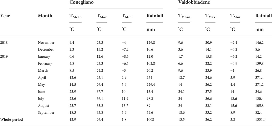
TABLE 2. Monthly weather data of the two sites during the experiment. T_Mean is mean air temperature (°C), T_Max is maximum air temperature (°C), T_Min is minimum air temperature (°C), and rainfall is the monthly cumulated precipitation (mm).

FIGURE 2

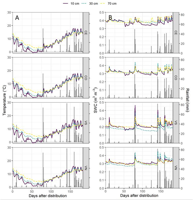
FIGURE 2. Soil temperature (°C) (A) and the soil water content (SWC, m³ m⁻³) (B) dynamics for the four monitoring stations at the three monitoring depths (10 cm, solid purple line; 30 cm, dotted green line; and 70 cm, dotted yellow line) with rainfall events (mm).

Glyphosate and AMPA concentrations in water

A total of 146 water samples were collected during the 6-month field experiment at the different depths in the four monitoring stations. In both experimental sites, discontinuous GLP and AMPA findings were observed in soil water as highlighted by the high variability between monitoring stations and depths in Figure 3. GLP in Conegliano was hardly detectable compared to Valdobbiadene. In Conegliano, GLP and AMPA concentrations were > LOQ for only seven and three out of 32 and 36 water samples (21.9% and 8.3%, in CE and CO, respectively), compared to 14 and 12 times out of 38 and 37 in Valdobbiadene (36.8% and 32.4%, in VS and VN, respectively).

FIGURE 3

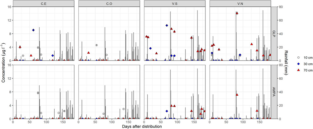
FIGURE 3. Glyphosate and AMPA detection in soil pore water samples in different monitoring stations and depths. Bars identify daily rainfall events. Data < LOQ are reported in the graphs equal to zero.

In the CE station (Figure 3), GLP was detected first at 70 cm depth (4.26 μg l⁻¹), 21 days after application, remaining below LOQ at 10 and 30 cm during the same period. At 30 days, GLP was detected only in the top layer (1.5 μg l⁻¹), followed by a maximum peak of 9.2 μg l⁻¹ 61 days at 30 cm depth. Afterward, GLP decreased to 1.5 μg l⁻¹ (119 days after contamination) at 30 cm depth and was no longer detected along the soil profile. Similar to CE, GLP in CO was detected first at 70 cm depth after some rain events (2.3 μg l⁻¹, 30 days after the distribution), then it was detected only in the surface layer until 54 (4.6 μg l⁻¹) and 84 (1.7 μg l⁻¹) days after herbicide spraying (Figure 3) and never at 30 cm. It should be noted that in both CE and CO, AMPA was found only at 15 cm from day 75.

Different GLP and AMPA dynamics were observed in Valdobbiadene, being mostly found at 70 cm depth since the beginning of the monitoring activities (Figure 3). In both VS and VN, GLP was found following the first rain events. In VN, GLP was found at 10 cm (1.8 μg l⁻¹), 30 cm (2.1 μg l⁻¹), and 70 cm depth (4.4 μg l⁻¹) 7 days after spraying, which increased up to 4.8 μg l⁻¹ at day 12. On the same day, GLP was 7.2 and 7.0 μg l⁻¹ at 70 cm depth in VS and was never detected at 10 cm. After a 3-day heavy rainfall event (February 1–3, 131.8 mm in total), GLP was found in VS and VN at 70 cm (Figure 3) at very high concentrations (9.4 and 14.1 μg l⁻¹, respectively), followed by a gradual reduction until 2.7 and 1.5 μg l⁻¹ at day 161. In VS, GLP in the intermediate layer increased up to 10.3 μg l⁻¹ 68 days after the distribution, followed by a reduction to 1.5 μg l⁻¹ (day 91) and its subsequent disappearance (<LOQ). Notably, AMPA was often found in VS since day 68 (30 cm) compared to VN where it was hardly detected but always in conjunction with GLP.

Values used for the calculation of AF are reported in Table 3. The risk of herbicide mobility to the groundwater was estimated according to the AF index; values were always zero regardless of the experimental sites, suggesting a low susceptibility to water contamination.

TABLE 3

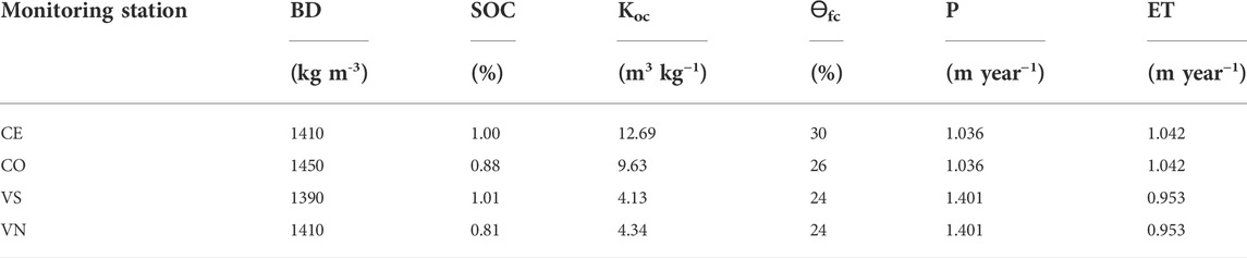
TABLE 3. Values and parameters are used to calculate AF. BD is bulk density, SOC is soil organic carbon, K_oc is the repartition coefficient between water and organic carbon, Ɵ_fc is the water content at field capacity, P is annual precipitation, and ET is annual evapotranspiration calculated from data recorded by the weather station from October 2018 to September 2019.

Concentration of glyphosate and AMPA formation in soil

Glyphosate and AMPA in soil were always detected in the surface layer (0–5 cm), while from 5 to 70 cm, they were found occasionally and randomly (Table 4). It follows that Eqs 2, 3 were only applied for the topsoil layer in both sites. Maximum GLP values were found one day after the application, with topsoil concentrations that ranged between 1018.9 μg kg⁻¹ in VN and 1279.6 μg kg⁻¹ in CO. After that, GLP concentrations sharply reduced until complete dissipation in all plots between day 133 and 182, while in VN it was still detected at 182 days. GLP residue in topsoil was well fitted by first-order exponential decay (Eq. 2), with R² > 0.94. In particular, the rate constants k varied between 0.016 and 0.025 days⁻¹ in Valdobbiadene and Conegliano, respectively. The lower k estimated in Valdobbiadene highlighted slower dissipation dynamics than in Conegliano (Figure 4 left, and Table 5), which had a constant rate 36% higher than that of the former. The formation–dissipation AMPA kinetics (Figure 4 right) was slightly different between Conegliano and Valdobbiadene. In the first case, the formation of AMPA was faster than its dissipation until day 30 in both CE and CO, when a peak in soil concentration reached 425.2 and 661.1 μg kg⁻¹, respectively. After day 30, the formation was slower and AMPA in soils decreased. In Valdobbiadene, maximum soil AMPA concentrations (Table 4) were observed at day 133 for both VS (311.6 μg kg⁻¹) and VN (420.4 μg kg⁻¹). The fitting model described the observed AMPA dynamics in Conegliano better (R² = 0.85) than in Valdobbiadene (R² = 0.80). The alpha (α) value and maximum occurrence time (t_max) in Conegliano were 0.017 and 21.2 days, respectively (Table 5), while a slower (α = 0.008 days⁻¹) and delayed (t_max = 28.8 ± 0.2 days, on average) AMPA dissipation was found in Valdobbiadene. Related to the deeper soil layers, GLP was found only six out of 68 times, e.g., at 5–20 cm in CE and CO the day after the distribution (Table 4). After 91 days it was found at 40–70 cm in CE and at 40–50 cm in VN. At the same depth in the latter, AMPA was also detected (64.6 μg kg⁻¹). At day 133, GLP was found at 40–50 cm only in VS, while more than 300 days after the herbicide distribution, GLP and AMPA were not detected. Related to the deeper soil layers, GLP was found only six out of 68 times, e.g., at 5–20 cm in CE and CO the day after the distribution (Table 4). After 91 days it was found at 40–70 cm in CE and 40–50 cm in VN. At the same depth in the latter, AMPA was also detected (64.6 μg kg⁻¹). At day 133, GLP was found at 40–50 cm only in VS, while more than 300 days after the herbicide distribution, GLP and AMPA were not detected.

TABLE 4

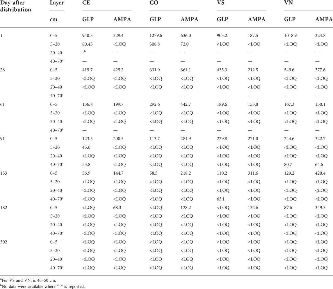
TABLE 4. GLP and AMPA (µg kg⁻¹) detection in soil layers at different times and depths after the distribution.

FIGURE 4

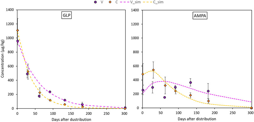
FIGURE 4. Dissipation dynamics of GLP in the topsoil layer (0–5 cm) for the the two sites fitted with the SFO equation (on the left, Eq. 2) and formation/dissipation dynamics of AMPA in the topsoil layer for the two sites fitted in Eq. 3 (on the right). Dots refer to experimental concentrations (orange for Conegliano and purple for Valdobbiadene) and lines refer to fitted dynamics.

TABLE 5

TABLE 5. Rate constants (k and α), coefficient of determination (R²), and root mean square error (RMSE) as indicators of the goodness of fit of glyphosate and AMPA with dissipation times (DT₅₀ in days) in the topsoil layer (0–5 cm) of the four monitoring stations. C_M (µg kg⁻¹) is the concentration of the parent molecule that is transformed to AMPA at the initial time and t_max (days) is the time at maximum AMPA occurrence.

Adsorption of glyphosate

Regarding the analysis of GLP adsorption, a good accuracy of the Freundlich equation (Table 6) was found at all depths and in the different experimental sites (R² always ≥0.95). The estimated 1/n was always <1 indicating that nonlinear adsorption occurred. The averaged 1/n was fixed at 0.76 ± 0.03 to calculate the averaged adsorption coefficient (K_f-mean). In general, K_f-mean varied between sites and depths showing a weaker GLP adsorption in Valdobbiadene than in Conegliano soils, the average being K_f-mean = 35.6 ± 3.4 and 140.7 ± 25.2, respectively. According to soil depth, the lowest K_f-mean was always observed in the topsoil layer (on average, 25.4 ± 3.2 and 112.9 ± 34.2 in Valdobbiadene and Conegliano, respectively), which gradually increased with depth until average values of 42.8 ± 1.8 and 174.7 ± 68.0 below 40 cm were obtained. Within Conegliano, the adsorption was broadly variable between monitoring stations, with K_f-mean ranging between 147.0 and 242.7 in CE and between 78.7 and 106.7 in CO. Lower variability was observed in Valdobbiadene, K_f-mean being in the 28.7–44.6 range in VS and 22.2–41.0 in VN.

TABLE 6

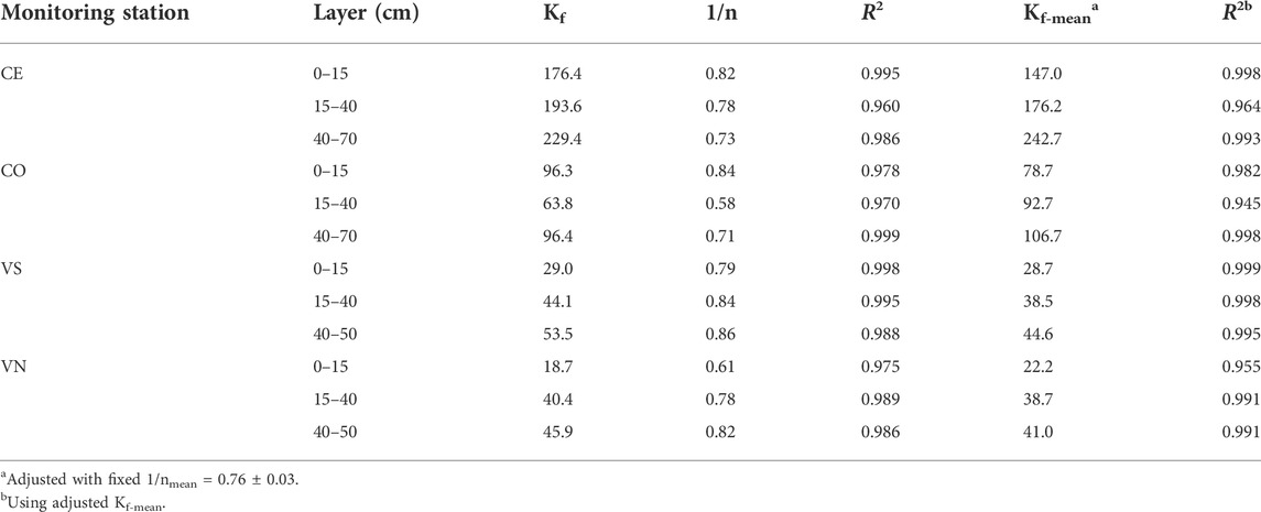
TABLE 6. Freundlich equation parameters for GLP (K_f, n, and K_f-mean) and coefficients of determination (R²) for different monitoring stations and soil layers. K_f and K_f-mean are reported in μg^1–1/n (ml)^1/n g⁻¹.

Al and Fe contents in the soil

Poorly ordered Fe and Al oxides (Fe_Ox and Al_Ox, respectively, mg kg⁻¹) generally decreased with depth in Conegliano (Table 7). Lower values were observed in the topsoil layer than deeper ones for Al_Ox in both VS and VN and for Fe_Ox in VS Conegliano had Fe_Ox always below 2000 mg kg⁻¹, with the lowest values being found in CO along the whole soil profile (761.9 ± 201.8 mg kg⁻¹). In contrast, Valdobbiadene had a relatively higher Fe_Ox content, being 2538.3 ± 310.0 mg kg⁻¹ in VS and 2648.1 ± 86.6 mg kg⁻¹ in VN. Differently, Al_Ox was always found at lower concentrations than Fe_Ox and with similar concentrations between experimental sites. The Al_Ox concentration was on average 279.7 ± 13.4 and 293.6 ± 15.6 mg kg⁻¹ in Conegliano and Valdobbiadene, respectively, and ranged between a minimum of 217.7 mg kg⁻¹ at the 40–70-cm layer in CO and a maximum of 354.6 mg kg⁻¹ at the 15–40-cm layer in VS Iron and aluminum chelated to soil organic matters (Fe_Som and Al_Som) were at similar average concentrations between the two sites, although different compositions were found with a variation of depth. Both SOM-chelated metals in the Conegliano site increased with depth (+26% and +65% on average in the deepest layer compared to the shallower one for Fe_Som and Al_Som, respectively), while in Valdobbiadene, they decreased at deeper soil depths (−47% and −20% for Fe_Som and Al_Som, respectively). In Conegliano, CE had the highest amount of Fe_Som and Al_Som (on average 606.37 ± 44.32 and 648.03 ± 91.99 mg kg⁻¹, respectively). Furthermore, in Conegliano at 40–70 cm, Al_Som was predominant with respect to Fe_Som (+26% as average between the two stations). An inverse trend was found in Valdobbiadene. Here, both monitoring stations had similar Fe_Som contents in the 0–15-cm layer (359 ± 16.80 mg kg⁻¹), decreasing to 224.1 in VS and 148.7 mg kg⁻¹ in VN at 40–70 cm depth. Furthermore, Al_Som had about half the concentration of that of Fe_Som. The ratio between Fe_Som and Al_Som and the SOC content is also reported in Table 7.

TABLE 7

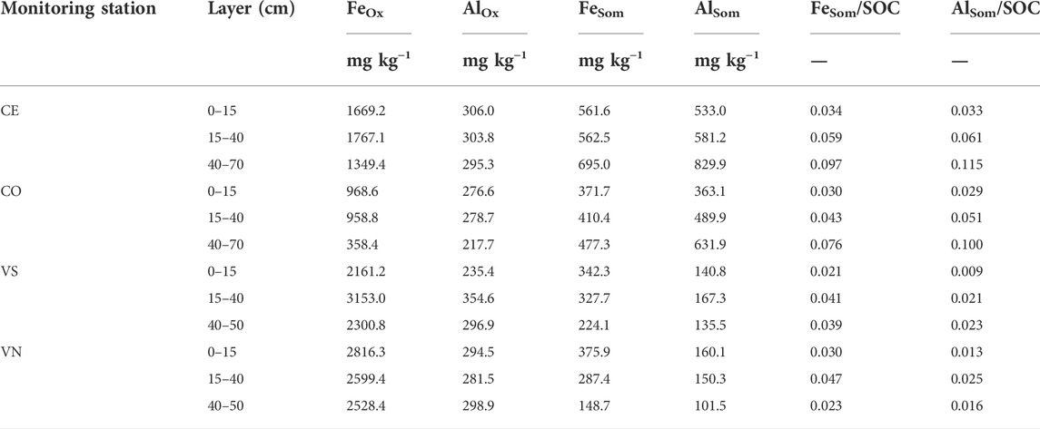
TABLE 7. Oxalate-extractable (Fe_Ox and Al_Ox) and SOM-chelated (Fe_Som and Al_Som) Al and Fe contents (mg kg⁻¹) in the four monitoring stations and soil depths. The ratio between Fe_Som and Al_Som and the SOC content (mg kg⁻¹) is also reported.

Discussion

During the 10-month monitoring experiment following herbicide distribution, GLP and AMPA were regularly detected in the topsoil 0–5 cm layer, while they were hardly found in the deeper layers or in pore water samples. However, some rapid transport of GLP to the deepest layers occurred, being first detected at 70 cm depth in water samples, e.g., just after 21 days in CE and 7 days in both VS and VN. GLP was first detected more superficially at 10 and 30 cm depths only after 7 (VN) and 30 days (CE). These results suggest the likely occurrence of GLP bypass flow in the intermediate layers as also reported by others (Vereecken, 2005; Stone and Wilson, 2006; Borggaard and Gimsing, 2008) and in turn a limited equilibration between predominantly vertical transport movement—probably only a small fraction of the total pore space was involved—and lateral mixing with the surrounding matrix (Jarvis et al., 2016) that reduced filter and buffer functions of soil. This was not the case for CO (Figure 3 and Table 4), emphasizing that local-specific conditions governing solute movement can occur. It should be noted that the high-frequency GLP and AMPA were found in the deepest layer, in both VS and VN, up to water concentrations of 14.1 and 9.4 and μg l⁻¹, respectively. This was likely emphasized using pan lysimeters that collected the percolation water even from the noncapillary macropores from the overlying layers. Here, GLP could have been sorbed onto soil particles (Piccolo et al., 1994; De Jonge et al., 2000), enhancing the concentration of the molecule in the suspension. It should be highlighted that the use of suction cups to intercept GLP concentration in pore water does not allow for the collection of colloid-transported molecules (Lapworth et al., 2005). Furthermore, experimental results of soil moisture in the deeper profiles (Figure 2B) highlighted differences in water and solute movement dynamics (Jarvis, 2007; Mencaroni et al., 2021) between the sites. Specifically, the soil moisture in CE and CO at 30 and 70 cm depth did not respond to rainfall events earlier than the shallower layer (Figure 3). In contrast, this dynamics was observed in VS and VN, which might support the occurrence of solute bypass (Graham and Lin, 2011). Estimates of GLP mobility according to the AF index seem to corroborate the previous results. Despite the AF index suggesting a low risk of groundwater contamination (AF always zero at each station), experimental findings demonstrated that some fast GLP vertical movement occurred. In fact, AF does not include the particular soil structure heterogeneity that might lead to site-specific solute bypass. Moreover, it does not account for single heavy rainfall events, which could have had an effect on moving the herbicide through the soil matrix down to 70 cm depth (Carretta et al., 2021b). Finally, the finding of GLP and AMPA below 30 cm can be due to herbicide interception by the aboveground vegetation, its following translocation into belowground tissues, and its likely release by dead roots below the topsoil (Laitinen et al., 2007).

The monitored experimental sites were characterized by grassland (Valdobbiadene) and grassed vineyard (Conegliano), which could have favored some movement of GLP (Alaoui, 2015) and in turn AMPA due to, e.g., an increase in macropores under long-term stabilized soil conditions. Regarding the role of SOC, contrasting results were reported in the literature to increase—or not increase—it (Vereecken, 2005). In our experiment, the SOC content was mainly split between the topsoil—with SOC values > 12.4 g kg⁻¹— and layers below 15 cm with values ≤ 9.6 g kg⁻¹, which reached a minimum of 5.8 g kg⁻¹ in the 40–50 cm layer in VS. A significant correlation between Freundlich adsorption coefficient and SOC was not found (Table 8), although negatively charged organic molecules would suggest the predominance of electrokinetically repulsive forces toward GLP, especially at alkaline soil pH conditions (Borggaard and Gimsing, 2008). In this context, the significant positive correlations between SOM-chelated Fe and Al and K_f-mean (r = 0.89 and 0.93, respectively, Table 8) indicated the occurrence of interactions between negatively charged functional groups in SOM and positively charged minerals with high surface areas, which likely mitigated unfavorable conditions for adsorption by creating bridges with the GLP phosphonic moiety (Morillo et al., 2000; Fink et al., 2016). Here, the high fraction of SOM-chelated iron and aluminum found in both sites increased along the soil profile despite the carbon content decreasing, as already observed by Bascomb (1968). The ratio between SOM-chelated metals and SOC (Fe_Som/SOC and Al_Som/SOC) was also investigated (Table 7). A high value of this ratio suggests that a large amount of Fe and Al are coupled with the SOM component, and vice versa, a low ratio indicates that SOM is associated with a low amount of Fe or Al. The relationship between Fe_Som/SOC and Al_Som/SOC and K_f-mean is reported in Figure 5. As the ratio increases, the sorption capacity is enhanced confirming the effect of cation bridges played by Fe and Al. This was especially observed for the Conegliano site, which had greater Fe_Som/SOC and Al_Som/SOC ratios than Valdobbiadene, and in turn higher K_f-mean. On the other hand, the significant positive correlation of K_f-mean with CEC (r = 0.72), silt, and clay (r = 0.74 and 70.81, respectively) and the negative one with sand (r = -0.88) (Table 8) corroborated the GLP affinity for fine soil particles mainly due to cation bridging (Kah and Brown, 2007). Dollinger et al. (2015) predicted GLP sorption using pedotransfer functions, identifying clay, CEC, and SOC as K_f predictors in a multiple regression analysis. Using the same equation, R² = 0.48 (p = 0.01) between experimental and estimated K_f-mean was found (Table 9). The implementation of multiple regression parameterization accounting for all experimental soil parameters analyzed here revealed that clay and CEC were significant predictors of GLP sorption capacity, similar to the findings by Dollinger et al. (2015). By contrast, SOC was not selected, while both amorphous and SOM-chelated metals were significant predictors of K_f-mean leading to an overall R² = 0.97 (Table 9), thus corroborating the major role of amorphous Fe and Al oxide surfaces (Rampazzo et al., 2013; Maqueda et al., 2017) over SOM-chelated ones.

TABLE 8

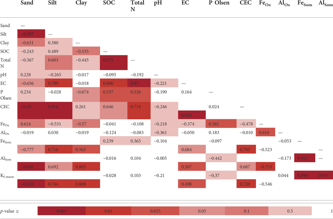
TABLE 8. Pearson correlation coefficient matrix between sorption coefficients and soil properties in the four monitoring stations (N = 13). Different colors indicate a range of p-values.

FIGURE 5

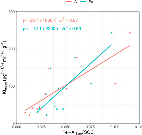
FIGURE 5. Regression lines with coefficient of determination between Al_Som/SOC (orange dots) and K_f-mean and between Fe_Som/SOC (blue triangles) and K_f-mean.

TABLE 9

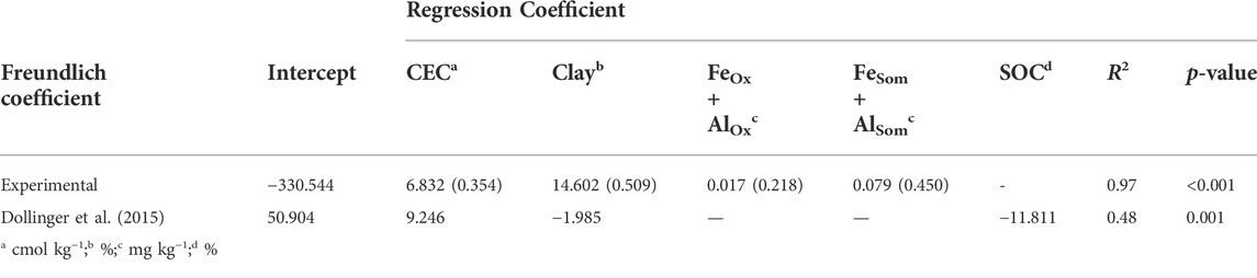
TABLE 9. Multiple linear regression analysis for estimation of Freundlich sorption coefficient (K_f-mean for experimental and K_f for Dollinger) according to soil parameters and Dollinger et al. (2015). Both unstandardized and standardized (in brackets) regression coefficients (p < 0.05) are reported.

The dissipation time (DT₅₀) has been calculated (reported in Table 5) using Eq. 6 despite the low amount of sampling points in the first 30 days of the experiment. For AMPA, the rate coefficient α was used instead of k in Eq. 6. Estimated dissipation of GLP was 28 days in Conegliano and 43 days in Valdobbiadene, highlighting a significant variability between the two experimental sites. In contrast, a low variability within each site can be hypothesized, which is supported by the low variability of both pedogenetic (ARPAV, 2008) and experimental physicochemical analysis of the sites. Nevertheless, expanding these data to other soils of the Prosecco area with the same pedogenesis must be carefully evaluated because other factors (e.g., soil management) might strongly affect the dissipation dynamics. In general, DT₅₀ calculated according to first-order kinetics were slightly longer than that calculated, e.g., in the laboratory in a clay loam agricultural French Cambisol (7–26 days) (Mamy et al., 2016), in Argentinian agricultural field trials on silt to loam soils (9–38 days) (Bento et al., 2019; Okada et al., 2019) and in Danish sandy soils (16.9 days) (Bergström et al., 2011). In Italian agricultural fields, GLP DT₅₀ was 9–18 days and 99–250 days for AMPA according to different tillage managements (Carretta et al., 2021a). To our knowledge, few data are available in the literature about AMPA kinetics, which here averaged 67 days as similarly reported by Bento et al. (2019) (55–71 days) and (Bergstrom et al., 2011) (35–60 days). The GLP dissipation and transformation to AMPA occurred without any lag phase corroborating previous findings (e.g., Nguyen et al., 2018), although the degradation rate could vary widely. From our results, dissipation dynamics of GLP and AMPA in the topsoil under field conditions was the combination of water percolation, runoff, and degradation phenomena, while erosion events were negligible in experimental monitoring stations in flat areas being characterized by dense grass cover. Hence, GLP and AMPA dissipation/formation in the soil might be predominantly affected by microorganism degradation (Sprankle et al., 1975) rather than water movement (e.g., enhanced leachability). In this context, greater cumulative rainfall and lower dissipation rate constants were detected in Valdobbiadene than in Conegliano, confirming that heavier rainfall events did not lower the persistence of the molecule in soil by, e.g., leaching or runoff. Higher fine particles, CEC, and Fe and Al oxides in the soil would suggest greater sorption, an enhanced GLP and AMPA protection against degradation (Bergström, 1990), and in turn higher DT₅₀ in Conegliano than Valdobbiadene. In contrast, estimated DT₅₀ values were the opposite, suggesting that other factors had likely contributed to GLP and AMPA dissipation, or conservation, in soils. For instance, it is likely that some specific weather conditions contributed to differences between the two experimental sites. After 61 days, both GLP and AMPA concentrations were affected by a sharp reduction, mainly in the Valdobbiadene soil, and then, at the following sampling date, they increased again (Figure 4). It is to be noted that snowfall (∼1 cm) in January 2019 and low temperatures (Table 2) were recorded in the experimental sites, which could have frozen GLP and AMPA in the dead weed, and then released them from the plant material to the soil with the gradual increase in temperature (Laitinen et al., 2009).

Conclusion

The glyphosate application in two soils of the Prosecco DOCG wine-growing area confirmed the general GLP and AMPA low mobility and highlighted the pivotal role of Fe and Al as key factors to mitigate the repulsive forces, especially when complexed with organic molecules. It is therefore suggested to study their content better to predict GLP dynamics. Between experimental sites, Conegliano showed a faster dissipation (about 28 days for GLP, 42 for AMPA) in the 0–5 cm of soil and higher sorption to soils (depth average K_f-mean = 140.6) than Valdobbiadene (about 43 days for GLP, 92 for AMPA; depth average K_f-mean = 35.6). However, a reduced soil-filtering capacity was observed during intense rain events as emphasized by some preferential movements due to likely well-structured soil conditions that could increase groundwater vulnerability to contamination. It follows that an in-depth water and solute monitoring activity at a site-specific level is required after the careful definition of homogeneous areas of the Prosecco terroir, which goes beyond the estimate of only leachability indexes that do not include the heterogeneity of soil structure and hydraulic properties. This phenomenon might be further exacerbated due to repeated GLP applications in cultivated areas or under particular pedoclimatic conditions that could increase GLP and AMPA dissipation times. Therefore, sparing use of GLP is suggested, which might be planned after evaluation of the most appropriate weather conditions.

Data availability statement

The original contributions presented in the study are included in the article/Supplementary Material; further inquiries can be directed to the corresponding author.

Author contributions

NDF, FM, GZ, and PS: conception and design of the study. MM: data collection, sample preparation, laboratory and statistical analyses, and preparation of the first draft of the manuscript. AC: laboratory analysis. PS: funding acquisition. All authors contributed to the manuscript, and they have revised, read, and approved the submitted version.

Funding

This research received funding from the project SWAT (Subsurface Water quality and Agricultural pracTices monitoring) UNI-IMPRESA 2017, C.I.R. Centro di Idrologia D. Tonini.

Acknowledgments

The authors thank the project partners Alto Trevigiano Servizi and Piave Servizi for the funding and support during the experimental setup. Special thanks to the University of Padova for supporting the acquisition of the TSQ Quantiva mass spectrometer by 2015/CPDB15489 funding.

Conflict of interest

The authors declare that the research was conducted in the absence of any commercial or financial relationships that could be construed as a potential conflict of interest.

Publisher’s note

All claims expressed in this article are solely those of the authors and do not necessarily represent those of their affiliated organizations, or those of the publisher, the editors, and the reviewers. Any product that may be evaluated in this article, or claim that may be made by its manufacturer, is not guaranteed or endorsed by the publisher.

Supplementary material

The Supplementary Material for this article can be found online at: https://www.frontiersin.org/articles/10.3389/fenvs.2022.971931/full#supplementary-material

SUPPLEMENTARY FIGURE S1 | Glyphosate concentration in μg L^‐1 in and out the pore water samplers with the identity line (1:1) as reference.

References

Ahuja, K., and Raeat, A. (2017). Glyphosate market size by application (conventional crops, GM crops), industry analysis report, regional outlook, application potential, price trends, competitive market share & forecast, 2016 – 2024. Delaware, USA: Selbyville.

Google Scholar

Alaoui, A. (2015). Modelling susceptibility of grassland soil to macropore flow. J. Hydrol. X. 525, 536–546. doi:10.1016/j.jhydrol.2015.04.016

CrossRef Full Text | Google Scholar

Antier, C., Kudsk, P., Reboud, X., Ulber, L., Baret, P. V., and Messéan, A. (2020). Glyphosate use in the European agricultural sector and a framework for its further monitoring. Sustainability 12, 5682. doi:10.3390/su12145682

CrossRef Full Text | Google Scholar

Arpav, (2019). Carta dei suoli 1:250.000. Agenzia Reg. Prev. Prot. Ambient. del veneto., 156.

Google Scholar

Arpav, (2008). Carta dei suoli della Provincia di Treviso 1:50.000. Agenzia Reg. Prev. Prot. Ambient. del veneto., 350.

Google Scholar

Arpav, (2020). Principali variabili meteorologiche (1994-2019). Agenzia Reg. Prev. Prot. Ambient. del veneto.

Google Scholar

Bascomb, C. L. (1968). Distribution of pyrophosphate-extractable iron and organic carbon in soils of various groups. J. Soil Sclence. 19, 251–268. doi:10.1111/j.1365-2389.1968.tb01538.x

CrossRef Full Text | Google Scholar

Bento, C. P. M., van der Hoeven, S., Yang, X., Riksen, M. M. J. P. M., Mol, H. G. J., Ritsema, C. J., et al. (2019). Dynamics of glyphosate and AMPA in the soil surface layer of glyphosate-resistant crop cultivations in the loess Pampas of Argentina. Environ. Pollut. 244, 323–331. doi:10.1016/j.envpol.2018.10.046

PubMed Abstract | CrossRef Full Text | Google Scholar

Bento, C. P. M., Yang, X., Gort, G., Xue, S., van Dam, R., Zomer, P., et al. (2016). Persistence of glyphosate and aminomethylphosphonic acid in loess soil under different combinations of temperature, soil moisture and light/darkness. Sci. Total Environ. 572, 301–311. doi:10.1016/j.scitotenv.2016.07.215

PubMed Abstract | CrossRef Full Text | Google Scholar

Bergström, L., Börjesson, E., and Stenström, J. (2011). Laboratory and lysimeter studies of glyphosate and aminomethylphosphonic acid in a sand and a clay soil. J. Environ. Qual. 40, 98–108. doi:10.2134/jeq2010.0179

PubMed Abstract | CrossRef Full Text | Google Scholar

Bergström, L. (1990). Use of lysimeters to estimate leaching of pesticides in agricultural soils. Environ. Pollut. 67, 325–347. doi:10.1016/0269-7491(90)90070-S

PubMed Abstract | CrossRef Full Text | Google Scholar

Bittelli, M., Andrenelli, M. C., Simonetti, G., Pellegrini, S., Artioli, G., Piccoli, I., et al. (2019). Shall we abandon sedimentation methods for particle size analysis in soils? Soil Tillage Res. 185, 36–46. doi:10.1016/J.STILL.2018.08.018

CrossRef Full Text | Google Scholar

Blake, R., and Pallett, K. (2018). The environmental fate and ecotoxicity of glyphosate. outlook. pest Man. 29, 266–269. doi:10.1564/v29_dec_08

CrossRef Full Text | Google Scholar

Borggaard, O. K., and Gimsing, A. L. (2008). Fate of glyphosate in soil and the possibility of leaching to ground and surface waters : A review. Pest Manag. Sci. 456, 441–456. doi:10.1002/ps.1512

PubMed Abstract | CrossRef Full Text | Google Scholar

Carles, L., Gardon, H., Joseph, L., Sanchís, J., Farré, M., and Artigas, J. (2019). Meta-analysis of glyphosate contamination in surface waters and dissipation by biofilms. Environ. Int. 124, 284–293. doi:10.1016/j.envint.2018.12.064

PubMed Abstract | CrossRef Full Text | Google Scholar

Carretta, L., Cardinali, A., Marotta, E., Zanin, G., and Masin, R. (2019). A new rapid procedure for simultaneous determination of glyphosate and AMPA in water at sub μg/L level. J. Chromatogr. A 1600, 65–72. doi:10.1016/j.chroma.2019.04.047

PubMed Abstract | CrossRef Full Text | Google Scholar

Carretta, L., Cardinali, A., Onofri, A., Masin, R., and Zanin, G. (2021a). Dynamics of glyphosate and aminomethylphosphonic acid in soil under conventional and conservation tillage. Int. J. Environ. Res. 15, 1037–1055. doi:10.1007/s41742-021-00369-3

CrossRef Full Text | Google Scholar

Carretta, L., Masin, R., and Zanin, G. (2021b). Review of studies analysing glyphosate and aminomethylphosphonic acid (AMPA) occurrence in groundwater. Environ. Rev. 30, 88–109. –22. doi:10.1139/er-2020-0106

CrossRef Full Text | Google Scholar

Consorzio di Tutela DOCG Conegliano Valdobbiadene (2019). Protocollo Viticolo del Conegliano Valdobbiadene Prosecco DOCG. Available at: http://repositorio.unan.edu.ni/2986/1/5624.pdf.

Google Scholar

Dal Ferro, N., Piccoli, I., Berti, A., Polese, R., and Morari, F. (2020). Organic carbon storage potential in deep agricultural soil layers: Evidence from long-term experiments in northeast Italy. Agric. Ecosyst. Environ. 300, 106967. doi:10.1016/j.agee.2020.106967

CrossRef Full Text | Google Scholar

De Jonge, H., De Jonge, L. W., and Jacobsen, O. H. (2000). [14C]glyphosate transport in undisturbed topsoil columns. Pest Manag. Sci. 56, 909–915. doi:10.1002/1526-4998(200010)56:10<909::AID-PS227>3.0

CrossRef Full Text | Google Scholar

De Jonge, H., De Jonge, L. W., Jacobsen, O. H., Yamaguchi, T., and Moldrup, P. (2001). Glyphosate sorption in soils of different pH and phosphorus content. Soil Sci. 166, 230–238. doi:10.1097/00010694-200104000-00002

CrossRef Full Text | Google Scholar

de Paz, J. M., and Rubio, J. L. (2006). Application of a GIS-AF/RF model to assess the risk of herbicide leaching in a citrus-growing area of the Valencia Community, Spain. Sci. Total Environ. 371, 44–54. doi:10.1016/j.scitotenv.2006.07.018

PubMed Abstract | CrossRef Full Text | Google Scholar

De Polo, A., Rossi, S., Bulfoni, I., Bardin, A., Gentili, D., and Cinquetti, S. (2019). From the traces in the wells of the urban aqueduct network to the subsequent prohibition of the use of glyphosate: The case of an area of high-intensity wine production in the province of treviso, Veneto. Ig. Sanita Pubbl. 75, 451–460.

PubMed Abstract | Google Scholar

Dollinger, J., Dagès, C., and Voltz, M. (2015). Glyphosate sorption to soils and sediments predicted by pedotransfer functions. Environ. Chem. Lett. 13, 293–307. doi:10.1007/s10311-015-0515-5

CrossRef Full Text | Google Scholar

EFSA (2015). Conclusion on the peer review of the pesticide risk assessment of the active substance glyphosate. EFSA J. 13. doi:10.2903/j.efsa.2015.4302

CrossRef Full Text | Google Scholar

EFSA (2017). Peer review of the pesticide risk assessment of the potential endocrine disrupting properties of glyphosate. EFSA J. 15, e04979. doi:10.2903/j.efsa.2017.4979

PubMed Abstract | CrossRef Full Text | Google Scholar

Fink, J. R., Inda, A. V., Tiecher, T., and Barrón, V. (2016). Iron oxides and organic matter on soil phosphorus availability. Cienc. Agrotec. 40, 369–379. doi:10.1590/1413-70542016404023016

CrossRef Full Text | Google Scholar

Gairhe, B., Liu, W., Batuman, O., Dittmar, P., Kadyampakeni, D., and Kanissery, R. (2021). Environmental fate and behavior of the herbicide glyphosate in sandy soils of Florida under citrus production. Front. Environ. Chem. 2, 1–9. doi:10.3389/fenvc.2021.737391

CrossRef Full Text | Google Scholar

Graham, C. B., and Lin, H. S. (2011). Controls and frequency of preferential flow occurrence: A 175-event analysis. Vadose zone J. 10, 816–831. doi:10.2136/vzj2010.0119

CrossRef Full Text | Google Scholar

Grossman, B. R., and Reinsch, T. G. (2002). “2.1 bulk density and linear extensibility,” in Methods soil anal. Part 4 phys. Methods. Editors J. H. Dane, and C. G. Topp (Madison, Wisconsin: Soil Science Society of America), 201–228. doi:10.2136/sssabookser5.4.c9

CrossRef Full Text | Google Scholar

Ibrahim, H. M., and Ali, A. T. M. (2020). Assessment of the environmental risk of pesticides leaching at the watershed scale under arid climatic conditions and low recharge rates. Water 12, 418. doi:10.3390/w12020418

CrossRef Full Text | Google Scholar

Jarvis, N. J. (2007). A review of non-equilibrium water flow and solute transport in soil macropores: Principles, controlling factors and consequences for water quality. Eur. J. Soil Sci. 58, 523–546. doi:10.1111/j.1365-2389.2007.00915.x

CrossRef Full Text | Google Scholar

Jarvis, N., Koestel, J., and Larsbo, M. (2016). Understanding preferential flow in the vadose zone: Recent advances and future prospects. Vadose Zone J. 15, vzj2016.09.0075. doi:10.2136/vzj2016.09.0075

CrossRef Full Text | Google Scholar

Kah, M., and Brown, C. D. (2007). Prediction of the adsorption of ionizable pesticides in soils. J. Agric. Food Chem. 55, 2312–2322. doi:10.1021/jf063048q

PubMed Abstract | CrossRef Full Text | Google Scholar

Kjær, J., Olsen, P., Ullum, M., and Grant, R. (2003). Vadose zone processes and chemical transport leaching of glyphosate and amino-methylphosphonic acid from Danish agricultural field sites. J. Environ. Qual. 34, 608–620. doi:10.2134/jeq2005.0608

CrossRef Full Text | Google Scholar

Kodešová, R., Kočárek, M., Kodeš, V., Drábek, O., Kozák, J., and Hejtmánková, K. (2011). Pesticide adsorption in relation to soil properties and soil type distribution in regional scale. J. Hazard. Mat. 186, 540–550. doi:10.1016/j.jhazmat.2010.11.040

CrossRef Full Text | Google Scholar

Laitinen, P., Rämö, S., Nikunen, U., Jauhiainen, L., Siimes, K., and Turtola, E. (2009). Glyphosate and phosphorus leaching and residues in boreal sandy soil. Plant Soil 323, 267–283. doi:10.1007/s11104-009-9935-y

CrossRef Full Text | Google Scholar

Laitinen, P., Rämö, S., and Siimes, K. (2007). Glyphosate translocation from plants to soil - does this constitute a significant proportion of residues in soil? Plant Soil 300, 51–60. doi:10.1007/s11104-007-9387-1

CrossRef Full Text | Google Scholar

Laitinen, P., Siimes, K., Eronen, L., Rämö, S., Welling, L., Oinonen, S., et al. (2006). Fate of the herbicides glyphosate, glufosinate-ammonium, phenmedipham, ethofumesate and metamitron in twoFinnish arable soils. Pest Manag. Sci. 62, 473–491. doi:10.1002/ps.1186

PubMed Abstract | CrossRef Full Text | Google Scholar

Lapworth, D., Gooddy, D., Harrison, I., Kim, A., and Vane, C. (2005). Colloidal phase transport of pesticides: A review with special reference to major UK aquifers. Br. Geol. Surv., Internal Report, IR/05/131, 31. Available at: http://nora.nerc.ac.uk/4490/.

Google Scholar

Lewis, K., and Tzilivakis, J. (2017). Development of a data set of pesticide dissipation rates in/on various plant matrices for the pesticide properties database (PPDB). Data 2 28. doi:10.3390/data2030028

CrossRef Full Text | Google Scholar

Mamy, L., Barriuso, E., and Gabrielle, B. (2016). Glyphosate fate in soils when arriving in plant residues. Chemosphere 154, 425–433. doi:10.1016/j.chemosphere.2016.03.104

PubMed Abstract | CrossRef Full Text | Google Scholar

Maqueda, C., Undabeytia, T., Villaverde, J., and Morillo, E. (2017). Behaviour of glyphosate in a reservoir and the surrounding agricultural soils. Sci. Total Environ. 593–594, 787–795. doi:10.1016/j.scitotenv.2017.03.202

PubMed Abstract | CrossRef Full Text | Google Scholar

McKeague, J., Brydon, J., and Miles, N. (1971). Differentiation of forms of extractable iron and aluminum in soils. Soil Sci. Soc. Am. J. 35, 33–38. doi:10.2136/sssaj1971.03615995003500010016x

CrossRef Full Text | Google Scholar

Mencaroni, M., Dal Ferro, N., Redcliffe, D., and Morari, F. (2021). Preferential solute transport under variably saturated conditions in a silty loam soil: Is the shallow water table a driving factor? J. Hydrol. X. 602, 126733. doi:10.1016/j.jhydrol.2021.126733

CrossRef Full Text | Google Scholar

Morillo, E., Undabeytia, T., and Maqueda, C. (1997). Adsorption of glyphosate on the clay mineral montmorillonite: Effect of Cu(II) in solution and adsorbed on the mineral. Environ. Sci. Technol. 31, 3588–3592. doi:10.1021/es970341l

CrossRef Full Text | Google Scholar

Morillo, E., Undabeytia, T., Maqueda, C., and Ramos, A. (2000). Glyphosate adsorption on soils of different characteristics. Chemosphere 40, 103–107. doi:10.1016/S0045-6535(99)00255-6

PubMed Abstract | CrossRef Full Text | Google Scholar

Neumann, G., Kohls, S., Landsberg, E., Stock-Oliveira Souza, K., Yamada, T., and Römheld, V. (2006). Relevance of glyphosate transfer to non-target plants via the rhizosphere. J. Plant Dis. Proctectio, Suppl. 969, 963–969. doi:10.1016/j.psychres.2016.04.036

CrossRef Full Text | Google Scholar

Nguyen, N. K., Dörfler, U., Welzl, G., Munch, J. C., Schroll, R., and Suhadolc, M. (2018). Large variation in glyphosate mineralization in 21 different agricultural soils explained by soil properties. Sci. Total Environ. 627, 544–552. doi:10.1016/j.scitotenv.2018.01.204

PubMed Abstract | CrossRef Full Text | Google Scholar

Noori, J. S., Dimaki, M., Mortensen, J., and Svendsen, W. E. (2018). Detection of glyphosate in drinking water: A fast and direct detection method without sample pretreatment. Sensors Switz. 18, 2961. doi:10.3390/s18092961

PubMed Abstract | CrossRef Full Text | Google Scholar

Nowack, B., and Stone, A. T. (2006). Competitive adsorption of phosphate and phosphonates onto goethite. Water Res. 40, 2201–2209. doi:10.1016/j.watres.2006.03.018

PubMed Abstract | CrossRef Full Text | Google Scholar

OECD (2000). Test No. 106: Adsorption -- desorption using a batch equilibrium method. OECD Guidel. Test. Chem., 1–44. doi:10.1787/9789264069602-en

CrossRef Full Text | Google Scholar

Okada, E., Costa, J. L., and Bedmar, F. (2016). Adsorption and mobility of glyphosate in different soils under no-till and conventional tillage. Geoderma 263, 78–85. doi:10.1016/j.geoderma.2015.09.009

CrossRef Full Text | Google Scholar

Okada, E., Costa, J. L., and Bedmar, F. (2019). Glyphosate dissipation in different soils under No-till and conventional tillage. Pedosphere 29, 773–783. doi:10.1016/S1002-0160(17)60430-2

CrossRef Full Text | Google Scholar

Ololade, I. A., Oladoja, N. A., Oloye, F. F., Alomaja, F., Akerele, D. D., Iwaye, J., et al. (2014). Sorption of glyphosate on soil components: The roles of metal oxides and organic materials. Soil Sediment Contam. Int. J. 23, 571–585. doi:10.1080/15320383.2014.846900

CrossRef Full Text | Google Scholar

Otto, S., Riello, L., Düring, R. A., Hummel, H. E., and Zanin, G. (1997). Herbicide dissipation and dynamics modelling in three different tillage systems. Chemosphere 34, 163–178. doi:10.1016/S0045-6535(96)00356-6

CrossRef Full Text | Google Scholar

Perri, M. T., Cassiani, G., Gervasio, I., Deiana, R., and Binley, A. (2012). A saline tracer test monitored via both surface and cross-borehole electrical resistivity tomography: Comparison of time-lapse results. J. Appl. Geophy. 79, 6–16. doi:10.1016/j.jappgeo.2011.12.011

CrossRef Full Text | Google Scholar

Piccolo, A., Celano, G., Arienzo, M., and Mirabella, A. (1994). Adsorption and desorption of glyphosate in some european soils. J. Environ. Sci. Heal. B29 (6), 1105–1115. doi:10.1080/03601239409372918

CrossRef Full Text | Google Scholar

R Core Team (2020). R: A language and environment for statistical computing. Vienna, Austria: R Foundation for Statistical Computing. Available at: https://www.rstudio.com/wp-content/uploads/2015/03/ggplot2-cheatsheet.pdf%5Cnhttps://www.rstudio.com/wp-content/uploads/2015/06/ggplot2-french.pdf.

Google Scholar

Rampazzo, N., Todorovic, G. R., Mentler, A., and Blum, W. E. H. (2013). Adsorption of glyphosate and aminomethylphosphonic acid in soils. Int. Agrophys. 27, 203–209. doi:10.2478/v10247-012-0086-7

CrossRef Full Text | Google Scholar

Rao, P. S. C., Hornsby, A. G., and Jessup, R. E. (1985). “Indices for ranking the potential for pesticide contamination of groundwater,” in Proceedings of the Soil and Crop Science Society of Florida, University of Florida, Gainesville, FL, 1–8.

Google Scholar

Sidoli, P., Baran, N., and Angulo-Jaramillo, R. (2016). Glyphosate and AMPA adsorption in soils: Laboratory experiments and pedotransfer rules. Environ. Sci. Pollut. Res. 23, 5733–5742. doi:10.1007/s11356-015-5796-5

PubMed Abstract | CrossRef Full Text | Google Scholar

Sprankle, P., Meggitt, W. F., and Penner, D. (1975). Adsorption, mobility and microbial degradation of glyphosate in the soil. Weed Sci. 23, 229–234. doi:10.1017/s0043174500052929

CrossRef Full Text | Google Scholar

Stone, W. W., and Wilson, J. T. (2006). Preferential flow estimates to an agricultural tile drain with implications for glyphosate transport. J. Environ. Qual. 35, 1825–1835. doi:10.2134/jeq2006.0068

PubMed Abstract | CrossRef Full Text | Google Scholar

Vereecken, H. (2005). Mobility and leaching of glyphosate: A review. Pest Manag. Sci. 61, 1139–1151. doi:10.1002/ps.1122

PubMed Abstract | CrossRef Full Text | Google Scholar

Viti, M. L., Alves, P. A. T., Mendes, K. F., Pimpinato, R. F., Guimaraes, A. C. D., and Tornisello, V. L. (2019). Translocation and root exudation of glyphosate by urochloa brizantha and its transport on sugarcane and citrus seedlings. Planta Daninha 37, 1–8. doi:10.1590/s0100-83582019370100030

CrossRef Full Text | Google Scholar

Wrb, I. W. G. (2014). International soil classification system for naming soils and creating legends for soil maps. Italy: FAO Rome.World reference base for soil resources 2014

Google Scholar

Zovi, F., Camporese, M., Hendricks Franssen, H. J., Huisman, J. A., and Salandin, P. (2017). Identification of high-permeability subsurface structures with multiple point geostatistics and normal score ensemble Kalman filter. J. Hydrol. X. 548, 208–224. doi:10.1016/j.jhydrol.2017.02.056

CrossRef Full Text | Google Scholar