Using existing infrastructure as ground control points to support citizen science coastal UAS monitoring programs

Recent publications have described the ability of citizen scientists to conduct unoccupied aerial system (UAS) flights to collect data for coastal management. Ground control points (GCPs) can be collected to georeference these data, however collecting ground control points require expensive surveying equipment not accessible to citizen scientists. Instead, existing infrastructure can be used as naturally occurring ground control points (NGCPs), although availably of naturally occurring ground control point placement on such infrastructure differs from published best practices of ground control point placement. This study therefore evaluates the achievable accuracy of sites georeferenced with naturally occurring ground control points through an analysis of 20 diverse coastal sites. At most sites naturally occurring ground control points produced horizontal and vertical root mean square errors (RMSE) less than 0.060 m which are similar to those obtained using traditional ground control points. To support future unoccupied aerial system citizen science coastal monitoring programs, an assessment to determine the optimal naturally occurring ground control point quantity and distribution was conducted for six coastal sites. Results revealed that generally at least seven naturally occurring ground control points collected in the broadest distribution across the site will result in a horizontal and vertical root mean square errors less than 0.030 m and 0.075 m respectively. However, the relationship between these placement characteristics and root mean square errors was poor, indicating that georeferencing accuracy using naturally occurring ground control points cannot be optimized solely through ideal quantity and distribution. The results of these studies highlight the value of naturally occurring ground control points to support unoccupied aerial system citizen science coastal monitoring programs, however they also indicate a need for an initial accuracy assessment of sites surveyed with naturally occurring ground control points at the onset of such programs.

1 Introduction

Coastal environments are broadly used by humans to support infrastructure, provide ecosystem services, and supply areas for housing and recreation (de Groot et al., 2012; Mehvar et al., 2018). These uses can be impacted by natural system dynamics such as erosion and sediment transport resulting from storms and changing water levels (Zhang et al., 2004; Phillips and Jones, 2006). Effective coastal management must therefore balance these human uses with coastal changes as well as develop proactive strategies that help build resilience to future changes (Gopalakrishnan et al., 2016; Dastgheib et al., 2018; Masselink and Lazarus, 2019; Molino et al., 2020; Rumson et al., 2020). Developing effective coastal management and coastal resilience strategies rely on high spatio-temporal resolution coastal morphology data (Nichols et al., 2019; Rumson et al., 2020; Huang et al., 2021). These data are needed to assess vulnerability to existing infrastructure (Bove et al., 2020), delineate property ownership (Morton and Speed, 1998), design and evaluate shoreline management actions such as armoring or beach nourishment (Gares et al., 2006), and track general coastal morphology changes (Turner et al., 2016; Theuerkauf et al., 2021). While the need and utility for such datasets is well articulated both in the scientific literature as well as in community and beach master plans, the complexity of gathering, analyzing, and implementing the data can create a barrier for communities who lack the personnel or financial resources to collect these data. Citizen science-based mapping programs that utilize new technologies such as unoccupied aerial systems (UAS) present an opportunity to broaden participation in data-driven management to such communities, however, the accuracy and utility of such datasets must be critically evaluated.

Aerial imagery and digital elevation models (DEMs) are two of the primary datasets coastal managers can utilize to document coastal changes (Huang et al., 2021). Prior to the recent proliferation of UAS, aerial imagery was primarily acquired by occupied aircrafts and satellites. Unfortunately, low-cost or publicly available satellite imagery such as that from the Sentinel-2 satellite may lack the desired resolution (e.g., 10 m GSD; Sentinel-2 Data Access and Products Fact Sheet, 2015) necessary for coastal management, while the high cost of occupied aircraft imagery limits the collection frequency (typically annually). Throughout most of the 20th century, coastal elevation data were collected along profiles using the rod and level technique (Emery, 1961). As more advanced methods such as differential Real-Time Kinematic GPS (RTK-GPS) deployed through backpack or ATV surveys became established in the 1990s, researchers have been able to frequently generate DEMs over large spatial extents (Harley et al., 2011; Lee et al., 2013). RTK-GPS surveys require interpolation between mapped transects however, limiting accuracy over complex topography (e.g., Theuerkauf and Rodriguez, 2012). With the advent of airborne LiDAR, researchers can collect elevation models at high resolutions over large and complex areas (Kidner et al., 2004; Jakubowski et al., 2013), although high cost also limits its use for frequent surveys. Terrestrial LiDAR can be deployed more frequently (O’Dea et al., 2019) but is limited by the spatial extent of the surveys. UAS represent the most recent advance in coastal surveying, as such technology are capable of generating aerial imagery and DEMs through a single survey and are more cost and time-efficient to deploy than previous survey methods (Mancini et al., 2013; Turner et al., 2016; Nikolakopoulos et al., 2019).

Geospatial datasets generated from UAS are derived by implementing photogrammetric structure-from-motion (SFM) algorithms on a series of overlapping offset images collected by UAS. These algorithms match common features in overlapping images to create a network of tie points used to reconstruct objects in 3-dimensional space (Westoby et al., 2012; James et al., 2017). This network of tie points can then be used to generate data products including DEMs and aerial imagery comprised of a mosaic of the original drone images (known as an orthomosaic). These data products are initially created in an arbitrary coordinate system however and require additional information to be accurately georeferenced, which is necessary to compare these data products to existing datasets. Georeferencing of UAS-SFM surveys is commonly conducted using ground control points (GCPs). In most cases, these points are physical markers with a high contrast checkered pattern placed around the scene and surveyed directly prior to the flight using RTK-GPS. The user identifies the location and coordinates of the GCPs in the images which allows the SFM software to optimize the estimates of the camera position, orientation, and internal parameters. This process defines a coordinate system and scale of the tie point network, as well as reducing systematic errors across the site (James et al., 2017). In addition to GCPs, check points (CPs) are surveyed and input into the SFM software in the same manner as GCPs but are not used in the error reduction and georeferencing process. Instead, the CPs are used as independent reference points to estimate the accuracy of the scene reconstruction at a given location.

While GCPs can greatly increase the accuracy of UAS-SFM derived data products, GCP effectiveness largely depends on their quantity and distribution throughout the site. As a result, there is a growing body of literature providing guidance on the ideal placement characteristics of GCPs. For sites less than 40 ha, studies have found that maximum achievable horizontal (XY) and vertical (Z) root mean square errors (RMSE) of 0.02–0.05 m and 0.04–0.10 m were reached with 5–20 and 9–20 GCPs respectively (Agüera-Vega et al., 2017; Martínez-Carricondo et al., 2018; Oniga et al., 2018; Manfreda et al., 2019; Meinen and Robinson, 2020; Yu et al., 2020; Zimmerman et al., 2020; Santana et al., 2021). These recommendations are likely site specific however, as environmental variables such as surface texture and morphology may effect survey accuracy (Westoby et al., 2012; Eltner et al., 2015). Studies evaluating the spatial distribution of GCPs found that at a minimum, GCPs should be placed around the perimeter of the site to minimize error (Martínez-Carricondo et al., 2018). This error can then be further decreased, especially in the vertical direction by evenly distributing GCPS throughout the site (Martínez-Carricondo et al., 2018; Santana et al., 2021). Zimmerman et al. (2020) tested distributions in a coastal environment and found GCPs placed at the corners of the rectangular study area, with adequate cross shore coverage, and at the minimum and maximum elevations minimized errors throughout the site. Conversely, studies have found that GCPs without adequate coverage can lead to inflated errors (Martínez-Carricondo et al., 2018; Santana et al., 2021). For example, concentrating all GCPs in the center or in one corner of the site.

The ease of UAS surveys, as well as the growing body of literature supporting their accuracy, have led to widespread use of UAS for coastal monitoring. They are now frequently implemented for scientific and engineering studies (Casella et al., 2020) and have recently been introduced as a tool for coastal monitoring by citizen scientists (e.g., Pucino et al., 2021; Theuerkauf et al., 2022). These citizen science programs train volunteer UAS pilots to periodically survey coastal areas in their communities. The image sets they collect are sent to institutions with the capacity and expertise to process the imagery into data products that can be used by the communities for coastal management. While clearly beneficial for scientists and communities alike, these networks pose a challenge to traditional GCP collection as citizen scientists are not equipped with RTK-GPS and cannot survey GCPs immediately prior to their flights.

Pucino et al. (2021) addresses this challenge by equipping each citizen scientist pilot with a set of “Smart GCPs” which have a high accuracy differential GPS system built into the survey marker. While effective, these “Smart GCPs” are costly and require additional effort on behalf of the citizen scientists to effectively deploy, retrieve, and maintain. Theuerkauf et al. (2022) addresses this challenge by utilizing existing infrastructure such as corners of park benches, parking stripes, manhole covers, or other static objects as GCPs (Figure 1A). These naturally occurring ground control points or NGCPs, can be surveyed at the onset of a monitoring program and used in lieu of traditional GCPs for the extent of the monitoring period. This method reduces project cost and survey effort compared to “Smart GCPs”, thus allowing for broader participation in the monitoring network for communities across a range of socio-economic settings. The accuracy of sites surveyed with NGCPs must be critically evaluated however, as the opportunities for NGCP placement are often restricted to stable upland structures, failing to adequately cover the dynamic coastal area where monitoring is needed. As a result, opportunities to place these NGCPs may drastically differ from the quantity and/or distribution of GCPs recommended in the literature, therefore presenting a challenge for deriving accurate data products for coastal research and management.

FIGURE 1

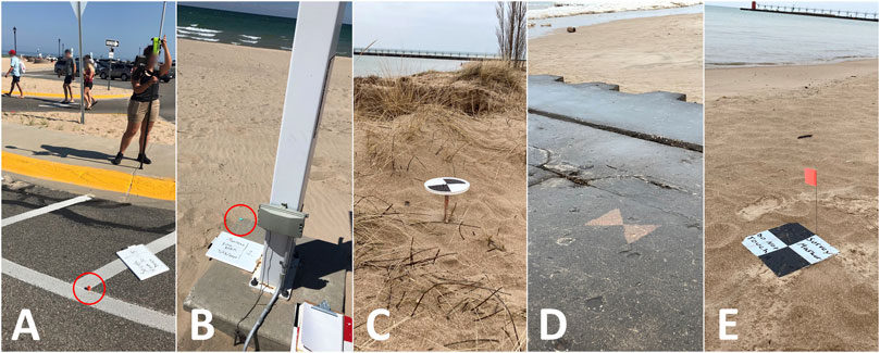
FIGURE 1. Examples of all types of NGCPs and CPs included in study. (A) Natural ground control point (NGCP), (B) NGCP surveyed on concrete block in the backshore that could become unusable if covered by sediment deposition, (C) Semipermanent NGCP mounted on a metal pole, (D) Semipermanent NGCP spraypainted onto concrete, (E) Check point (CP) surveyed on a temporary checkered high contrast marker. Red circles indicate the location of the NGCP where applicable.

Given the challenges with NGCPs placement, the purposes of this study are to: 1) Evaluate the ability of NGCPs to generate high accuracy data through an accuracy assessment of 20 coastal sites ranging in size and morphology and 2) Contribute to the literature on optimal GCP quantity and distribution by developing best practices for placing NGCPs in coastal environments through a case study in the Great Lakes. Through these investigations, we seek to demonstrate the utility of NGCPs for citizen science surveys and provide guidance for future UAS citizen science monitoring networks utilizing NGCPs.

2 Data and methods

2.1 Site selection and description

20 sites that are representative of the diversity of coastal morphologies found throughout the world, such as natural and developed beaches, bluffs, and foredunes, were examined in this study. These sites were in six different communities throughout the western Great Lakes region (Figure 2). At each of these 20 sites, a field survey was completed to establish NGCPs throughout the site. The sites ranged in size from approximately 0.1–3.0 ha and represent a range of morphologies from flat beaches varying only 1.25 m in elevation to steep bluffs varying over 20 m in elevation. In addition, these sites contain a variety of coastal infrastructure representing various opportunities for NGCP placements. The quantity and diversity of sites as well as the diversity of NGCP placement opportunities in this study represent an ideal opportunity to rigorously test the accuracy of NGCPs for georeferencing in coastal environments.

FIGURE 2

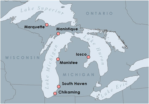
FIGURE 2. Location of the six communities participating in the Great Lakes citizen science UAS monitoring program established at Michigan State University. Communities include: Chikaming Township, City of South Haven, City of Manistee, City of Manistique, City of Marquette, and Iosco County.

Among these 20 sites, several had unique morphology and NGCP placement characteristics that are referred to in this publication. Sites with bluff morphology (Bluff-1, Bluff-2) are sites that only had NGCP placement opportunities at the top of the bluff landward of the crest, with no NGCPs placement locations lakeward of the bluff toe. Sites with backshore NGCP placement only (Backshore-2 and Backshore-1) refer to sites at the bottom of bluffs where the backshore makes up the entire site with no possible structures to survey as NGCPs. The resulting NGCPs at these sites needed to be mounted on poles and placed at the bluff toe where they were partially obscured by overhanging vegetation.

2.2 NGCP and CP placement

For each site, 3–12 NGCPs were established and surveyed using either a Trimble R10–2 or R12 RTK GPS system with 0.012 m (SD = 0.004 m) horizontal precision and 0.020 m (SD = 0.007 m) vertical precision. NGCPs were established on permanent objects throughout the site that could be easily identified in the UAS imagery. When possible, NGCPs were established with consideration to the broadest possible horizontal and vertical distributions as well as evenly distributed throughout the site in as suggested by the current literature on optimal GCP placement (Martínez-Carricondo et al., 2018; Zimmerman et al., 2020; Santana et al., 2021). At several of our sites where there were either no suitable locations to place NGCPs, or where the locations did not cover a large portion of the site, we installed semipermanent NGCPs (Figure 1). These semipermanent NGCPs were either spray painted survey markers on exposed concrete (Figure 1D), or a painted survey maker affixed to a 4-to-6-foot metal pole driven into the ground (Figure 1C). For this study we refer to both semipermanent NGCPs and NGCPs surveyed on objects already in the site as NGCPs unless explicitly stated otherwise. To assess horizontal and vertical measurement errors from the UAS-derived topography data, we surveyed CPs with the total amount per site depending on its size and topography. These check points were placed strategically to capture the maximum and minimum elevations of the site, the furthest lakeward extent of the site, around the perimeter of the site, the tops and bottoms of any berms of bluffs, and other evenly distributed locations throughout the site (Figure 3).

FIGURE 3

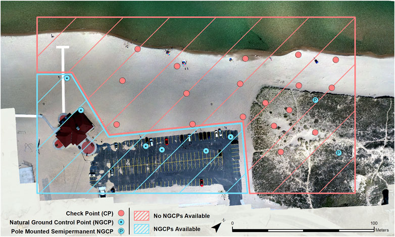
FIGURE 3. Example of accuracy assessment NGCP and CP placement scheme at P-5. Check points (CP) are shown as red points and natural ground control points (NGCPs) are shown as blue points. Pole mounted semipermanent NGCPs are shown as a blue point containing “P”. Portion of survey area where NGCPs can be surveyed are outlined in blue while portion of survey area where no NGCPs can be found are outlined in red.

2.3 Imagery collection

UAS surveys were conducted with either a DJI Phantom 4 Pro V2.0 or an Autel Evo II Pro quadcopter. The camera mounted on these UAS are similar with one inch, 5472 × 3648 20-megapixel sensors, and lenses with a similar f/2.8-f/11 aperture range, although with slightly different focal lengths. Since differing focal lengths result in varying spatial resolutions for a given flight height, flights were standardized by the ground footprint of the pixel, hereby referred to as the ground sampling distance (GSD) rather than by flight height. A GSD of 0.015 m was chosen, giving us the ability to confidently pick out the location of NGCPs. Recorded GSD varied between 0.013 and 0.020 m except for P-16 and P-1 which had a GSD of 0.007 and 0.008 m respectively, as these sites were surveyed before a GSD of 0.015 m was chosen. All surveys were conducted with 80% front and side overlap as recommended by Dandois et al. (2015), as well as nadir camera angle and auto settings for exposure, ISO, and aperture.

2.4 Structure from motion processing

All SFM models were created using Agisoft Metashape Professional Edition (Agisoft Metashape, 2021). Initial tie point matching was performed with the high accuracy setting and default parameters of 40,000 key point limit and 4,000 tie point limit. Adaptive model fitting was used which allows Metashape to automatically select which internal camera parameters are estimated based on their reliability estimates (Agisoft Metashape User Manual—Professional Edition, Version 1.6). Generally, more internal camera parameters can be reliably estimated when stronger geometry exists in the scene such as a building or bluff (Agisoft Metashape User Manual - Professional Edition, Version 1.6). Selecting which internal camera parameters to include is typically done on a site-specific basis, however due to the diversity of morphologies among our sites and the necessity of a streamlined workflow, the adaptive camera model fitting option was effective and efficient.

The locations of the NGCPs and CPs in each photo were selected with an estimated placement precision of one pixel (referred to as image coordinate marker accuracy in Metashape). The default image coordinate marker accuracy in Metashape is 0.5 pixels, however this value was increased to one pixel to account for the difficulty in identifying NGCP locations over traditional GCPs surveyed on checkered markers. Precision of the RTK-GPS for each NGCP and CP was set to the mean precision of all the RTK-GPS markers for a given survey site on a given day, which ranged from 0.007–0.025 m in the horizontal direction and 0.016–0.034 m in the vertical direction. The camera locations and internal parameters were optimized using all NGCPs with the adaptive camera model fitting parameter selected. Metashape then produces an estimate of the location of each CP based on the optimized tie point network which can be compared to the surveyed RTK-GPS locations to calculate a residual error (in meters) for each CP (Eq. 1).

2.5 Accuracy assessment

Accuracy of each of the 20 sites was determined by calculating the horizontal (XY), vertical (Z), and total XYZ error for each CP, as well as the horizontal, vertical, and total root mean square errors (RMSE) for each site using the following equations:

Eq. 1: Calculation of horizontal (A), vertical (B), and total (C) error for each CP.

${\mathit{E}\mathit{r}\mathit{r}\mathit{o}\mathit{r}}_{\mathit{X}\mathit{Y}}=\sqrt{{\left({\mathit{X}}_{\mathit{Mod}}–{\mathit{X}}_{\mathit{G}\mathit{P}\mathit{S}}\right)}^2+{\left({\mathit{Y}}_{\mathit{Mod}}–{\mathit{Y}}_{\mathit{G}\mathit{P}\mathit{S}}\right)}^2}(\mathrm{1A})$

${\mathit{E}\mathit{r}\mathit{r}\mathit{o}\mathit{r}}_{\mathit{Z}}=\sqrt{{\left({\mathit{Z}}_{\mathit{Mod}}–{\mathit{Z}}_{\mathit{G}\mathit{P}\mathit{S}}\right)}^2}(\mathrm{1B})$

${\mathit{E}\mathit{r}\mathit{r}\mathit{o}\mathit{r}}_{\mathit{X}\mathit{Y}\mathit{Z}}=\sqrt{{\left({\mathit{X}}_{\mathit{Mod}}–{\mathit{X}}_{\mathit{G}\mathit{P}\mathit{S}}\right)}^2+{\left({\mathit{Y}}_{\mathit{Mod}}–{\mathit{Y}}_{\mathit{G}\mathit{P}\mathit{S}}\right)}^2+{\left({\mathit{Z}}_{\mathit{Mod}}–{\mathit{Z}}_{\mathit{G}\mathit{P}\mathit{S}}\right)}^2}(\mathrm{1C})$

Eq. 2: Calculation of horizontal (A), vertical (B), and total (C) RMSE for all CPs in a site.

${\mathit{R}\mathit{M}\mathit{S}\mathit{E}}_{\mathit{X}\mathit{Y}}=\sqrt{\frac{{\sum }_{\mathit{i}=1}^{\mathit{n}}\left[{\left({\mathit{X}}_{\mathit{Mod}}–{\mathit{X}}_{\mathit{G}\mathit{P}\mathit{S}}\right)}^2+{\left({\mathit{Y}}_{\mathit{Mod}}–{\mathit{Y}}_{\mathit{G}\mathit{P}\mathit{S}}\right)}^2\right]}{\mathit{n}}}(\mathrm{2A})$

${\mathit{R}\mathit{M}\mathit{S}\mathit{E}}_{\mathit{Z}}=\sqrt{\frac{{\sum }_{\mathit{i}=1}^{\mathit{n}}{\left({\mathit{Z}}_{\mathit{Mod}}–{\mathit{Z}}_{\mathit{G}\mathit{P}\mathit{S}}\right)}^2}{\mathit{n}}}(\mathrm{2B})$

${\mathit{R}\mathit{M}\mathit{S}\mathit{E}}_{\mathit{X}\mathit{Y}\mathit{Z}}=\sqrt{\frac{{\sum }_{\mathit{i}=1}^{\mathit{n}}\left[{\left({\mathit{X}}_{\mathit{Mod}}–{\mathit{X}}_{\mathit{G}\mathit{P}\mathit{S}}\right)}^2+{\left({\mathit{Y}}_{\mathit{Mod}}–{\mathit{Y}}_{\mathit{G}\mathit{P}\mathit{S}}\right)}^2+{\left({\mathit{Z}}_{\mathit{Mod}}–{\mathit{Z}}_{\mathit{G}\mathit{P}\mathit{S}}\right)}^2\right]}{\mathit{n}}}(\mathrm{2C})$

where ${\left(X,Y,Z\right)}_{\mathit{Mod}}$ are the locations of the CPs derived from the SFM model and ${\left(X,Y,Z\right)}_{GPS}$ are the locations collected through the RTK-GPS survey.

Several additional tests were conducted to evaluate NGCP accuracy with possible scenarios. For example, the destruction of semipermanent NGCPs may be possible, as the spraypainted points can be washed away and pole mounted points can be moved by either human or natural disturbances. Additionally, several NGCPs were surveyed on concrete blocks on the backshore (backshore NGCPs) that may become unusable if covered by sediment deposition (Figure 1B). To assess the effect of the removal of the two types of semipermanent NGCPs as well as backshore NGCPs on site accuracy, we conducted an accuracy assessment on sites georeferenced excluding these three types of points. Additionally at bluff sites, we tested the inclusion of either one or two GCPs at the base of the bluff in the center and at either end respectively. This scenario evaluates how the accuracies of these sites may be improved beyond the accuracies achievable with solely NGCPs located at the bluff top.

The results of this accuracy assessment across the 20 sites are reported both in the horizontal and vertical direction. For example, data products that are accurately georeferenced in both the horizontal and vertical directions can be used to answer coastal management questions that require accurate elevations such as establishing patterns of sediment erosion and accretion, or delineating elevation based regulatory lines. However, data products that are only accurate in the horizontal directions may only be suitable to answer coastal management questions that do not require vertical elevations such as evaluating coastal areas for recreation or generating bluff recession rates by tracking the horizontal position of the bluff crest over time.

2.6 Optimal quantity and distribution of NGCPs

To determine the effect of NGCP quantity and distribution on the CP RMSE, a series of tests were conducted using different quantities and distributions of NGCPs on a subsample (n = 6) of the total sites (n = 20). These sites represent a variety of coastal morphologies and elevation ranges including low relief beaches (P-8 and P-10), moderate relief foredunes (P-9 and P-4), and high relief bluffs (Bluff-1, bluff-2) described in (Table 1).

TABLE 1

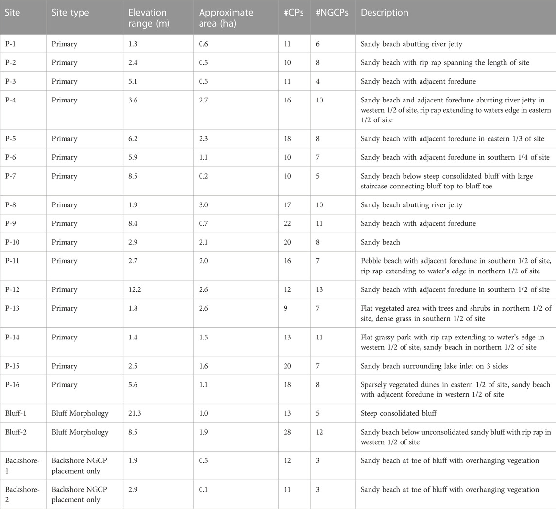
TABLE 1. Site type, elevation range, approximate area, quantity of NGCPs and CPs, and description of all 20 sites included in this study. Elevation range is calculated from the difference between the highest and lowest NGCP/CP within the site. Approximate area excludes excess area outside the boundaries of the site captured by NGCPs/CPs. #CP and # NGCP refer to the quantity of check points and natural ground control points surveyed at the site. Starred sites indicate those used for the analysis of NGCP quantity and distribution.

For each of the six subsampled sites, we randomly selected five different combinations of three NGCPs (the minimum required for georeferencing; James and Robson, 2012) from the total amount of NGCPs used for the site to be included in the camera optimization procedure. We then repeated this process for 50%, 75%, and 100% of the total quantity of NGCPs available for a total of 16 replications per site. The total number of NGCPs available to use at a given site for these tests varied from 8 to 11 depending on site size and structures available to be used for NGCPs. For each replication of NGCPs, we included any NGCPs not randomly selected to be included in the replication as additional CPs. A regression analysis comparing the quantity of NGCPs to the XY and Z RMSE for all sites combined was conducted with the results of these replications. For the purposes of the regression analysis, outliers greater than three times the interquartile range above the upper quartile or below the lower quartile were excluded. This removed six replications from the Z RMSE regression and three replications from the XY RMSE regression.

An exception to this procedure was implemented at the Bluff-1 site which is a high relief bluff with five NGCPs and five CPs along the stable land at the bluff top (landward of the bluff crest) and eight CPs at the bluff bottom (lakeward of the bluff toe). Because of the lack of NGCPs available to be used for replications, we included the five CPs at the top of the bluff as additional NGCPs for a total of 10 possible NGCPs to be used in the replications. The CPs at the top of the bluff were more accurate than those at the bottom of the bluff due to their relatively high proximity to the NGCPs at the bluff top. Therefore, increasing NGCPs removed these higher accuracy CPs, leading to a change in the proportion of CPs located at the bluff top vs. bluff bottom. To remove the effect of this varying proportion of higher accuracy CPs, we calculated CP RMSE using only the eight CPs located at the bluff bottom for all NGCP quantities, resulting in a more meaningful comparison of error between replications.

3 Results

3.1 Accuracy assessment

Figure 4 shows the results of the accuracy assessment for all 20 sites in the horizontal, vertical, and total directions. Of these 20 sites, those with either backshore NGCP placement only (Backshore-2 and Backshore-1) or with bluff morphology (Bluff-1, Bluff-2) are shown in the panel to the right, while the 16 remaining sites (referred to as primary sites) are shown to the left. At these 16 primary sites, Z RMSE was less than 0.060 m and in 14 out of the 16 sites, XY RMSE was less than 0.025 m. For the two sites with backshore NGCP placement only, Z RMSE was notably higher at 0.153 and 0.302 m while XY RMSE was similar to the primary sites, at 0.050 and 0.046 m. For the sites with bluff morphology, Bluff-2 had a Z RMSE higher than the primary sites but similar XY RMSE. For Bluff-1, Z RMSE was notably higher than any other site in the study and XY RMSE was slightly larger than all other sites. For both these sites, errors were concentrated at the base of the bluff, while errors at the top of the bluff were similar in magnitude to those found in the primary sites (Figure 5).

FIGURE 4

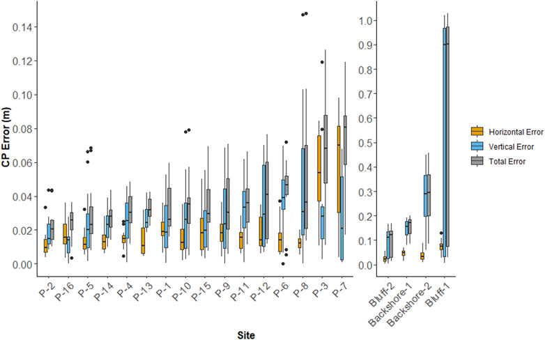
FIGURE 4. Distribution of check point error magnitudes (m) for all sites in the horizontal (orange), vertical (blue), and total (grey) directions. Boxes represent the interquartile range (IQR), whiskers represent points <1.5*(IQR) above or below the IQR, and dots represent points >1.5*(IQR) above or below the IQR. The left most 16 sites (P-1 à P-7) plotted using the left Y-axis from 0.00–0.15 m while the 4 sites on the right (Bluff-1 à Bluff-2) are plotted using the right Y-axis from 0.0–1.0 m.

FIGURE 5

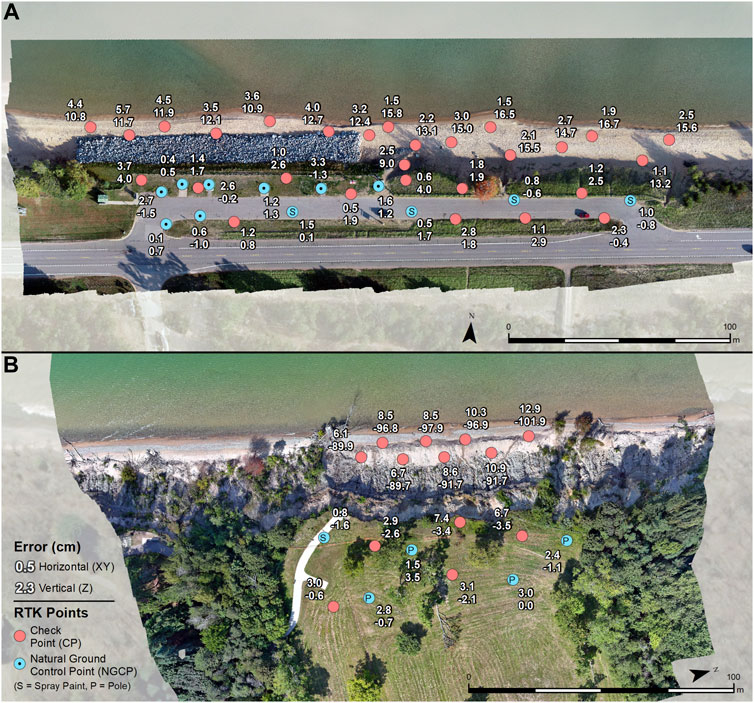
FIGURE 5. Check point (CP) and natural ground control point (NGCP) errors for sites with bluff morphology: Bluff-2 (A) and Bluff-1 (B). Red points indicate CP locations and blue points indicate NGCP locations. Semipermanent spraypainted NGCPs and semipermanent NGCPs mounted on poles are represented with an “S” and “P” respectively. Upper point labels show Horizontal (XY) error and lower labels show vertical (Z) error in cm.

For the two sites with bluff morphology, the addition of one or two additional GCPs located at the bottom of the bluff was evaluated. At Bluff-2, including one GCP placed at the bottom of the bluff decreased Z RMSE from 0.107 to 0.037 m and XY RMSE from 0.027 to 0.019. Adding an additional GCP at the base (2 total) produced a negligible additional reduction in RMSE. At the other bluff site, Bluff-1, one GCP at the bottom of the bluff decreased Z RMSE from 0.743 m to 0.228 m and slightly increased XY RMSE from 0.079 to 0.111 m. Including two GCPs at the base of the bluff further decreased Z RMSE to 0.143 and XY RMSE to 0.045 m.

At several sites, semipermanent NGCPs installed with either spray paint or metal poles as well as the easily covered backshore points were removed from the analyses to evaluate the impact on accuracy (Table 2). Of the 17 cases of reduced combinations of NGCPs, in eight cases removing these points had no effect (<0.025 m change) in either XY or Z RMSE. In seven cases, the removal of these points caused Z RMSE to increase, however it had little effect on the XY RMSE. The exception to these findings were the P-16 cases where removing these points caused an increase in XY RMSE and no effect on Z RMSE. At this site however, the semipermanent NGCPs increase the longshore spread of the NGCPs from roughly 25% to nearly 100%, while not contributing at all to the vertical spread of the NGCPs. Therefore, removing these semipermanent NGCPs caused a notable reduction in horizontal NGCP distribution without effecting vertical NGCP distribution.

TABLE 2

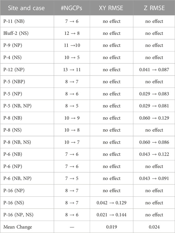
TABLE 2. Effect of removing easily destroyed natural ground control points (NGCPs) on check point horizontal (XY) and vertical (Z) RMSE. Cases of removed NGCPS include no backshore points (NB), no spraypainted points (NS), and no points mounted on metal poles (NP). Changes to RMSE <0.025 m are noted as “no effect” while all other changes are noted as “original value à new value”. Mean changes are calculated including the cases where removing points had no effect. All values are shown in meters.

3.2 Optimal quantity of NGCPs

Through the detailed analysis of NGCP quantity at the six subsampled sites, it was evident that the relationship between NGCP quantity and CP RMSE was different for Bluff-1 compared to the other five sites (P-4, Bluff-2, P-8, P-9, and P-10), thus Bluff-1 was removed from the regression analysis. This analysis revealed the relationship between XY and Z RMSE and quantity of NGCPs can be described using the following equations depicted by the blue lines in Figure 6.

FIGURE 6

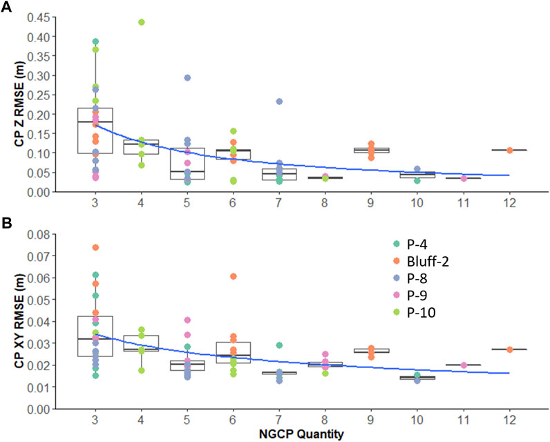
FIGURE 6. NGCP quantity vs. vertical (Z) RMSE (A) and horizontal (XY) RMSE (B). Each point represents the RMSE of a single replication for a given quantity of NGCPs, while point colors represent the site from which the RMSE is derived. Boxes represent the interquartile range (IQR), whiskers represent points <1.5*(IQR) above or below the IQR, and dots represent points >1.5*(IQR) above or below the IQR. Blue lines represent trend lines with the form: $\mathrm{y}=\mathrm{a}\mathrm{x}\mathrm{b}\mathrm{y}=\mathrm{a}\mathrm{x}\mathrm{b}$. Outliers greater than 3 times the interquartile range above the upper quartile of each NGCP quantity are not shown (top n = 6, bottom n = 3).

Eq. 3: Relationship between CP Z RMSE in meters and quantity of NGCPs (#NGCP).

$\mathit{Z}\mathit{R}\mathit{M}\mathit{S}\mathit{E}\left(\mathit{m}\right)=\mathbf{0.3468}{\left(\mathbf{\#}\mathit{N}\mathit{G}\mathit{C}\mathit{P}\right)}^{\mathbf{-}.\mathbf{8889}},{\mathit{R}}^{\mathbf{2}}=\mathbf{0.217},\mathit{P}-\mathit{V}\mathit{a}\mathit{l}\mathit{u}\mathit{e}=\mathbf{<}\mathbf{0.01}(3)$

Eq. 4: Relationship between CP XY RMSE in meters and quantity of NGCPs (#NGCP).

$\mathit{X}\mathit{Y}\mathit{R}\mathit{M}\mathit{S}\mathit{E}\left(\mathit{m}\right)=\mathbf{0.0488}{\left(\mathbf{\#}\mathit{N}\mathit{G}\mathit{C}\mathit{P}\right)}^{\mathbf{-}.\mathbf{4308}},{\mathit{R}}^{\mathbf{2}}=\mathbf{0.194},\mathit{P}-\mathit{V}\mathit{a}\mathit{l}\mathit{u}\mathit{e}=\mathbf{<}\mathbf{0.01}(4)$

In these five sites RMSE decreases in both the vertical and horizontal directions with the inclusion of additional NGCPs. Furthermore, the range of RMSE values for a given NGCP quantity is the greatest using only three NGCPs and generally decreases approaching the total number of NGCPs used. In the vertical direction in most cases, a Z RMSE less than 0.075 m was achieved using seven NGCPs or greater. The exception is in Bluff-2 (high relief bluff) which reached a Z RMSE of 0.080–0.128 m with six NGCPs and did not improve with additional NGCPs. In the horizontal direction, in most cases an XY RMSE of 0.045 m was achieved using only four NGCPs or greater, and in all cases an XY RMSE less than 0.030 m was achieved using seven NGCPs or greater. In both the horizontal and vertical directions, we observe a minimum achievable RMSE regardless of the number of NGCPs used at roughly 0.013 m and 0.025 respectively. While the mean RMSE across all replications decreases with additional NGCPs, for the majority of NGCP quantities used, some combinations of NGCPs achieve this minimum possible error. Contrary to other sites, at Bluff-1 (high relief bluff) which was not included in the regression analysis, Z RMSE increased from three to five NGCPs, and stabilized at a Z RMSE of 0.875–0.966 m with five or more NGCPs. In the horizontal direction, XY RMSE was largely unaffected by an increase in number of NGCPs, ranging from 0.038 to 0.111 m for all but one replication (Figure 7).

FIGURE 7

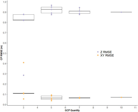
FIGURE 7. Bluff-1 NGCP quantity vs. RMSE. Purple points represent vertical (Z) RMSE, and orange points represent horizontal (XY) RMSE. Each point represents the RMSE of a single replication for a given quantity of NGCPs. Boxes represent the interquartile range (IQR), whiskers represent points <1.5*(IQR) above or below the IQR, and dots represent points >1.5*(IQR) above or below the IQR.

3.3 Optimal distribution of NGCPs

For each of the sites tested above, the distributions of NGCPs that produced the lowest and highest XYZ RMSE for each number of NGCPs tested above were also evaluated. The results varied by site with no clear relationship to site morphology. At P-4 (moderate relief foredune) and Bluff-2 (high relief bluff), for all quantities of NGCPs the distribution with the lowest XYZ RMSE had a broader or roughly equivalent horizontal spread of NGCPS than that of the distribution with the highest XYZ RMSE. The placement of NGCPS throughout these two sites did not allow us to isolate the effects of vertical vs. horizontal distributions however, as the NGCPs either lacked vertical variation (Bluff-2), or the NGCPs with the greatest vertical variation also had the greatest horizontal variation (P-4). Similar findings were observed at P-9 (low relief beach), although this site highlighted the importance of a broad horizontal as well as vertical distribution of NGCPs. This is especially evident when looking at the NGCP replications with the minimum number of NGCPs (3). In these replications, the distribution with broad Z spread and limited XY spread had a Z and XY RMSE of 0.037 and 0.100 m respectively, while the distribution with limited Z spread and broad XY spread had a Z and XY RMSE of 0.193 and 0.041 m respectively. This is contradicted however with the replications using 75% of the NGCPs (8). In these replications the XY and Z RMSEs between the two distributions was nearly identical at 0.019–0.025 m and 0.035–0.040 m respectively, but the vertical spread for the two distributions varied by over 4 m, a substantial portion of the 8.4 m total elevation range for the site.

In contrast, at two of the sites the smallest XYZ RMSE was not always achieved with the broadest NGCP distribution. For the minimum number of NGCPs (3) in P-10 (low relief beach), the less distributed NGCPs produced an XYZ RMSE of 0.237 m while the broadest distribution of NGCPs possible produced an XYZ RMSE of 2.310 m. With 75% of the NGCPs (6) however, the broadest distribution did produce the lowest XYZ errors. At P-8 (low relief beach), across all NGCP quantities the broadest distribution of NGCPs did not produce the lowest XYZ RMSE. This is evident in the replications using the minimum quantity of NGCPs (3) where the points clustered in one corner of the site produced an XYZ error of 0.064 m while the NGCPs spanning across the site produced an XYZ RMSE of 0.264 m (Figure 8). For replications using both 50% (5) and 75% (8) NGCPs, there was little difference in the spread between the points, however the XYZ RMSEs varied substantially from 0.039–0.294 m and 0.053–0.233 m respectively.

FIGURE 8

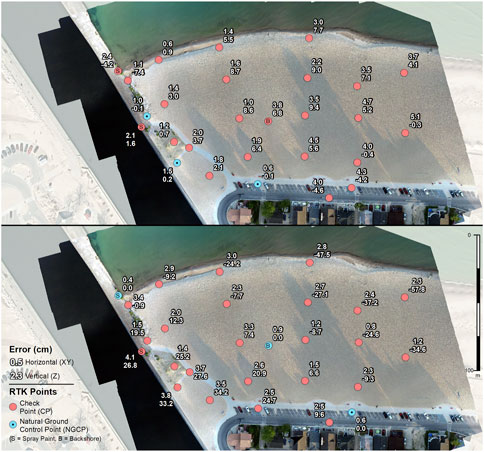
FIGURE 8. Check point (CP) and natural ground control point (NGCP) errors for replications of P-8 using three NGCPs. Top panel shows the distribution of NGCPs that resulted in the lowest CP total RMSE and bottom panel shows the distribution of NGCPs that resulted in the highest CP total RMSE. Red points indicate CP locations and blue points indicate NGCP locations. Spraypainted NGCPs and backshore NGCPs are represented with an “S” and “B” respectively. Upper point labels show horizontal (XY) error and lower labels show vertical (Z) error in cm.

4 Discussion

UAS surveys deployed by citizen scientists represent an opportunity to expand high quality coastal data to small, resource limited communities. The ability to georeference these sites using NGCPs reduces survey cost and effort, however the use of NGCPs may introduce errors reducing the utility of the derived data products for coastal management. This study determined that for almost all sites, using NGCPs produced vertical and horizontal errors comparable or slightly higher than errors obtained using traditional GCPs in coastal environment. The inclusion of 20 sites in this study gives further confidence to these findings, as a range of coastal morphologies and opportunities for NGCP placement were evaluated. At these accuracies, the data products generated from these citizen scientist networks can be used to support data driven management activities in resource limited communities.

The analysis conducted in this study to determine the optimal quantity and distribution of NGCPs to minimize RMSE of surveys also helps to support the expansion of the citizen science-UAS coastal monitoring programs. Through this analysis it was found that the accuracy of sites is only partially dependent on these placement characteristics. The effect of the quantity of NGCPs throughout sites can be modeled with Eqs. 3, 4 although the low R² squared values of these regressions indicate they should not be solely relied on to determine site error for a given quantity of NGCPs. In fact, the optimum achieved RMSE using all NGCPs available at a site can be achieved with as few as three NGCPs in some cases, highlighting the influence of other factors apart from NGCP quantity on check point RMSE (Figure 9). Furthermore, the relationship between NGCP quantity and RMSE is not consistent and appears to be partially influenced by site morphology. At bluff sites, for example, no additional change in accuracy was achieved with greater than five to six NGCPs, and in the case of one site (Bluff-1), more than three NGCPs counterintuitively resulted in an RMSE increase. In order to minimize error, our findings support previous work (Martínez-Carricondo et al., 2018; Zimmerman et al., 2020; Santana et al., 2021) that indicates NGCPs should be placed around the perimeter of the site in the broadest distribution possible in both the horizontal and vertical directions. In several cases notable deviations from this pattern were observed however, with the broadest distributions of NGCPs resulting in the higher errors compared to cases with more clustered NGCPs. The relationships between NGCP placement and data accuracy established during this study may not be applicable for stretches of coastline larger than our study sites (i.e., >250 m) and additional study is needed to evaluate the potential for scaling up these patterns.

FIGURE 9

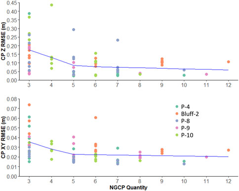
FIGURE 9. Piecewise regression of NGCP quantity vs. vertical (Z) RMSE (top) and horizontal (XY) RMSE (bottom). Each point represents the RMSE of a single replication for a given quantity of NGCPs, while point colors represent the site from which the RMSE is derived. Boxes represent the interquartile range (IQR), whiskers represent points <1.5*(IQR) above or below the IQR, and dots represent points >1.5*(IQR) above or below the IQR. Blue lines represent piecewise linear regression trend lines. Outliers greater than 3 times the interquartile range above the upper quartile of each NGCP quantity are not shown (top n = 6, bottom n = 3).

While these findings together provide basic recommendations about optimal NGCP quantity and distribution, it is clear there are other factors impacting site accuracy that cannot be described solely through these NGCP placement characteristics. One possible factor is the varying ability of NGCPs to be identified in the UAS images. Unlike traditional GCPs placed on identical checkered markers, objects used as NGCPs are placed on a variety of structures, leading to differences in image coordinate marker accuracy among the points. For example, at a 0.015 m GSD, misplacing the NGCP by two pixels could result in up to a 0.03 m variation in NGCP image coordinate marker accuracy. It is therefore possible that certain combinations of NGCPs contain points with higher or lower image coordinate marker accuracy, leading to the variations in CP error among different NGCP combinations.

Taking these findings into account, best practices for minimizing errors across sites surveyed by citizen scientists and georeferenced using NGCPs are presented. If both horizontal and vertical accuracy is desired, surveying at least seven NGCPs is recommended and will likely produce an Z RMSE of less than 0.075 m and XY RMSE less than 0.030 m. If only horizontal accuracy is required, the quantity of NGCPs can be reduced to four to obtain an RMSE less than 0.045 m. Surveying additional NGCPs is recommended however, as this may further decrease both horizontal and vertical accuracy as well as provide a buffer if any NGCPs are disturbed.

Any NGCPs used should be as broadly distributed across the site as possible in both the horizontal and vertical directions, but only if they can be sufficiently identified in photos. In other words, broadly placed NGCPs that are difficult to accurately identify may not be as useful as more clustered NGCPs that are easier to identify. Additionally, adding an abundance of NGCPs clustered in one portion of the survey area is discouraged, especially if this area is geographically dissimilar from the rest of the site, for example, at the top of a bluff.

Of the NGCPs used in this study, it is evident that consistent identification is easiest for those NGCPs with high color contrast placed on flat ground, for example, the corner of a white crosswalk on black asphalt. Conversely, placement of NGCPs on elevated geometric edges such as the top corner of a fence post or corner of a stair step should be avoided. In these cases, the varying angle of the object relative to the camera position will make it challenging to consistently identify the point. If placing points on geometric edges is unavoidable, structures with high color contrast between the vertical and horizontal surfaces of the structure are recommended. Without this contrast, when the vertical edge of the structure faces the camera, the geometric structure of the object can be difficult to resolve making NGCP identification inconsistent. If need be, shadows can be utilized as contrast considering time of day of the surveys. For example, if a citizen scientist expects to be conducting surveys in the morning with the Sun in the southeast, the northwest corner of the structure is the optimal choice for an NGCP, allowing a shadow to be cast across the vertical side of the structure, increasing contrast.

Placing an abundance of easy to identify NGCPs widely distributed throughout the survey site is often not possible. Therefore, an accuracy assessment using CPs placed throughout the site at the onset of a project should be conducted by the supporting institution for all citizen science UAS monitoring efforts. Without an accuracy assessment, the undocumented spatial errors of the data products could result in misleading data and less effective, cost-efficient, or even counterproductive coastal management actions. Conducting such an accuracy assessment will also allow a research team to update the check point errors across the site, should some NGCPs be destroyed. In this case, the georeferencing process can be repeated excluding the destroyed NGCPs, allowing researchers to determine the resulting change in accuracy and if a replacement effort for the lost NGCPs is necessary.

Challenges to georeferencing sites using NGCPs stem largely from sites either with bluff morphology, backshore NGCP placement only, or when NGCPs are destroyed. In these cases, vertical error may be higher than desired, potentially limiting their use for coastal management actions requiring accurate vertical elevation data such as volumetric calculations or delineating elevation-based jurisdictional boundaries (e.g., elevation-based ordinary high-water mark). However, in these cases our results indicate that horizontal error largely remains at levels comparable to the primary sites, allowing the data products from these challenging sites to be used for actions requiring only horizontal accuracy. For example, in many coastal states, erosion rates are used to evaluate erosion hazards associated with new and existing infrastructure (EGLE (2021), NYS-DEC). These rates are typically determined by comparing the horizontal position of a coastal erosion line over time, only requiring accuracy in the horizontal dimension. Additionally at bluff sites, these vertical inaccuracies can be reduced with the inclusion of even a single GCP placed at the bottom of the bluff. While this may not be possible using NGCPs, a single RTK enabled “smart GCP” marker could be used similar to those in Pucino et al. (2021) if access to the base of the bluff is possible for citizen scientists. While the inclusion of “smart GCPs” increases project cost and citizen science effort if used exclusively, a single smart GCP used for this purpose may provide a middle ground for maximizing accuracy while minimizing cost and effort.

While in these challenging cases the absolute accuracy of the data products may not be optimal, the fact that a consistent set of NGCPs are being used may facilitate high relative accuracy ideal for multitemporal change detection (Eltner et al., 2015). Future research is needed to fully understand the persistence of errors over time however, which can be effected by varying environmental conditions such as lighting, texture, and morphology change in response to sediment movement or coastal development. (Westoby et al., 2012; Eltner et al., 2015). Additionally, prior literature has found that check point error increases with greater distance to the nearest GCP (Gindraux et al., 2017; Sanz-Ablanedo et al., 2018). Therefore, if a coastal area expands, a previously conducted accuracy assessment may fail to account for increased errors at the water’s edge. Such expansion is common in freshwater environments such as the Great Lakes due to fluctuating water levels, or in marine environments where sediment supply outpaces sea level rise (Quinn, 2002; Hanrahan et al., 2010; van IJzendoorn et al., 2021). In most marine environments however, predicted coastal recession due to global sea level rise (Leatherman et al., 2000; Nicholls and Cazenave, 2010) may decrease the distance from NGCPs to the water’s edge, reducing check point errors at the shoreline.

5 Conclusion

In this study, the accuracy of UAS-SFM models georeferenced using NGCPs was evaluated at 20 coastal sites. At these sites, the use of NGCPs generally produced errors similar to those observed using traditional GCPs in similar environments. Higher vertical errors are observed however when NGCP placement is limited either by the morphology of the site or when previously surveyed NGCPs are moved or destroyed, reducing the ability of the derived data products to be used in management decisions requiring accurate elevations. In these cases, higher horizontal error was not observed thus preserving their utility for management decisions that only require horizontal accuracy. A detailed investigation on the optimal quantity and distribution of NGCPs needed to minimize error revealed that at most sites seven NGCPs were needed to consistently achieve vertical accuracies of less than 0.075 m Z RMSE and 0.030 m XY RMSE. If only horizontal accuracy is required is required, in most sites four NGCPs can be used to consistently obtain less than 0.045 m XY RMSE. In some sites however, the optimal accuracy can be obtained with far fewer GCPs, while in other sites additional NGCPs may increase error if they are restricted to areas morphologically dissimilar from the rest of the site. Generally, the broadest distribution of NGCPs both in the horizontal and vertical directions produced the lowest errors. Several notable exceptions were observed however were clustered NGCPs produced lower errors than broadly distributed NGCPS. While these findings together provide general guidelines to the optimal NGCP placement, the exceptions to these guidelines indicate that the accuracy of a site cannot be described purely through the quantity and distribution of NGCPs. Conducting an accuracy assessment of sites surveyed using NGCPs is therefore essential, as the lack of such an assessment can obscure errors throughout the site, leading to misinformed and less effective management decisions. The use of NGCPs in citizen-science based UAS coastal monitoring networks reduce survey cost and effort which facilitates the participation of smaller, resource limited communities in the networks. With the high-quality data generated from these studies, these communities are afforded the opportunity to conduct effective and timely data-driven management decisions.

Data availability statement

The raw data supporting the conclusions of this article will be made available by the authors, without undue reservation.

Author contributions

Funding for this research was acquired by EB and ET. ET, EB, and LR were responsible for conceiving of the study design. Data collection was undertaken by LR, ET, and EB. Image and data processing and analyses was led by LR under the supervision of ET and EB. LR wrote the manuscript under the supervision of ET and EB. ET and EB edited the manuscript and prepared it for submission.

Funding

This research was funded by a grant from the National Science Foundation’s Coastlines and People (CoPe) Program (Award Number: 1939979).

Acknowledgments

The authors would like to thank Ryan Poe and Megan Castro for assistance with field work and Everett Najarian for assistance with data processing. We also extend our gratitude to Elizabeth Mack for providing guidance and feedback on the manuscript. Additionally, we would like to thank the staff of MSU Remote Sensing and GIS Research and Outreach Services, especially Robert Goodwin, for project support and assistance.

Conflict of interest

The authors declare that the research was conducted in the absence of any commercial or financial relationships that could be construed as a potential conflict of interest.

Publisher’s note

All claims expressed in this article are solely those of the authors and do not necessarily represent those of their affiliated organizations, or those of the publisher, the editors and the reviewers. Any product that may be evaluated in this article, or claim that may be made by its manufacturer, is not guaranteed or endorsed by the publisher.

Supplementary material

The Supplementary Material for this article can be found online at: https://www.frontiersin.org/articles/10.3389/fenvs.2023.1101458/full#supplementary-material

References

Agisoft Metashape User Manual—Professional Edition, Version 1.6 (2020) Agisoft Metashape user manual—professional edition, version 1.6, 172. (n.d.).

Agisoft Metashape (2021). Agisoft Metashape (1.6.5) computer software.

Google Scholar

Agüera-Vega, F., Carvajal-Ramírez, F., and Martínez-Carricondo, P. (2017). Assessment of photogrammetric mapping accuracy based on variation ground control points number using unmanned aerial vehicle. Measurement 98, 221–227. doi:10.1016/j.measurement.2016.12.002

CrossRef Full Text | Google Scholar

Bove, G., Becker, A., Sweeney, B., Vousdoukas, M., and Kulp, S. (2020). A method for regional estimation of climate change exposure of coastal infrastructure: Case of USVI and the influence of digital elevation models on assessments. Sci. Total Environ. 710, 136162. doi:10.1016/j.scitotenv.2019.136162

PubMed Abstract | CrossRef Full Text | Google Scholar

Casella, E., Drechsel, J., Winter, C., Benninghoff, M., and Rovere, A. (2020). Accuracy of sand beach topography surveying by drones and photogrammetry. Geo-Marine Lett. 40 (2), 255–268. doi:10.1007/s00367-020-00638-8

CrossRef Full Text | Google Scholar

Dandois, J. P., Olano, M., and Ellis, E. C. (2015). Optimal altitude, overlap, and weather conditions for computer vision UAV estimates of forest structure. Remote Sens. 7 (10), 13895–13920. doi:10.3390/rs71013895

CrossRef Full Text | Google Scholar

Dastgheib, A., Jongejan, R., Wickramanayake, M., and Ranasinghe, R. (2018). Regional scale risk- informed land-use planning using probabilistic coastline recession modelling and economical optimisation: East coast of Sri Lanka. J. Mar. Sci. Eng. 6 (4), 120. doi:10.3390/jmse6040120

CrossRef Full Text | Google Scholar

de Groot, R., Brander, L., van der Ploeg, S., Costanza, R., Bernard, F., Braat, L., et al. (2012). Global estimates of the value of ecosystems and their services in monetary units. Ecosyst. Serv. 1 (1), 50–61. doi:10.1016/j.ecoser.2012.07.005

CrossRef Full Text | Google Scholar

EGLE - High Risk Erosion Areas: Program and Maps (2021) EGLE - high risk erosion areas: Program and maps. (n.d.). Retrieved August 9, 2021, from: https://www.michigan.gov/egle/0,9429,7-135-3311_4114-344443--,00.html.

Google Scholar

Eltner, A., Kaiser, A., Castillo, C., Rock, G., Neugirg, F., and Abellan, A. (2015). “Image-based surface reconstruction in geomorphometry – merits, limits and developments of a promising tool for geoscientists [Preprint],” in Cross-cutting themes: Digital Landscapes: Insights into geomorphological processes from high-resolution topography and quantitative interrogation of topographic data. doi:10.5194/esurfd-3-1445-2015

CrossRef Full Text | Google Scholar

Emery, K. O. (1961). A simple method of measuring beach profiles. Limnol. Oceanogr. 6 (1), 90–93. doi:10.4319/lo.1961.6.1.0090

CrossRef Full Text | Google Scholar

Gares, P. A., Wang, Y., and White, S. A. (2006). Using LIDAR to monitor a beach nourishment project at wrightsville beach, North Carolina, USA. J. Coast. Res. 22, 1206–1219. doi:10.2112/06A-0003.1

CrossRef Full Text | Google Scholar

Gindraux, S., Boesch, R., and Farinotti, D. (2017). Accuracy assessment of digital surface models from unmanned aerial vehicles’ imagery on glaciers. Remote Sens. 9 (2), 186. doi:10.3390/rs9020186

CrossRef Full Text | Google Scholar

Gopalakrishnan, S., Landry, C. E., Smith, M. D., and Whitehead, J. C. (2016). Economics of coastal erosion and adaptation to sea level rise. Annu. Rev. Resour. Econ. 8 (1), 119–139. doi:10.1146/annurev-resource-100815-095416

CrossRef Full Text | Google Scholar

Hanrahan, J. L., Kravtsov, S. V., and Roebber, P. J. (2010). Connecting past and present climate variability to the water levels of Lakes Michigan and Huron. Geophys. Res. Lett. 37 (1). doi:10.1029/2009GL041707

CrossRef Full Text | Google Scholar

Harley, M. D., Turner, I. L., Short, A. D., and Ranasinghe, R. (2011). Assessment and integration of conventional, RTK-GPS and image-derived beach survey methods for daily to decadal coastal monitoring. Coast. Eng. 58 (2), 194–205. doi:10.1016/j.coastaleng.2010.09.006

CrossRef Full Text | Google Scholar

Huang, X., Song, Y., and Hu, X. (2021). Deploying spatial data for coastal community resilience: A review from the managerial perspective. Int. J. Environ. Res. Public Health 18 (2), 830. doi:10.3390/ijerph18020830

PubMed Abstract | CrossRef Full Text | Google Scholar

Jakubowski, M. K., Guo, Q., and Kelly, M. (2013). Tradeoffs between lidar pulse density and forest measurement accuracy. Remote Sens. Environ. 130, 245–253. doi:10.1016/j.rse.2012.11.024

CrossRef Full Text | Google Scholar

James, M. R., and Robson, S. (2012). Straightforward reconstruction of 3D surfaces and topography with a camera: Accuracy and geoscience application. J. Geophys. Res. Earth Surf. 117 (F3). doi:10.1029/2011JF002289

CrossRef Full Text | Google Scholar

James, M. R., Robson, S., d’Oleire-Oltmanns, S., and Niethammer, U. (2017). Optimising UAV topographic surveys processed with structure-from-motion: Ground control quality, quantity and bundle adjustment. Geomorphology 280, 51–66. doi:10.1016/j.geomorph.2016.11.021

CrossRef Full Text | Google Scholar

Kidner, D. B., Thomas, M. C., Leigh, C., Oliver, J. R., and Morgan, C. G. (2004). Coastal monitoring with LiDAR: Challenges, problems, and pitfalls (M. Ehlers, F. Posa, H. J. Kaufmann, U. Michel, and G. De Carolis, Eds, 80). doi:10.1117/12.565648

CrossRef Full Text | Google Scholar

Leatherman, S. P., Zhang, K., and Douglas, B. C. (2000). Sea level rise shown to drive coastal erosion. Eos, Trans. Am. Geophys. Union 81 (6), 55–57. doi:10.1029/00EO00034

CrossRef Full Text | Google Scholar

Lee, J.-M., Park, J.-Y., and Choi, J.-Y. (2013). Evaluation of sub-aerial topographic surveying techniques using total station and RTK-GPS for applications in macrotidal sand beach environment. J. Coast. Res. 65 (10065), 535–540. doi:10.2112/SI65-091.1

CrossRef Full Text | Google Scholar

Mancini, F., Dubbini, M., Gattelli, M., Stecchi, F., Fabbri, S., and Gabbianelli, G. (2013). Using unmanned aerial vehicles (UAV) for high-resolution reconstruction of topography: The structure from motion approach on coastal environments. Remote Sens. 5 (12), 6880–6898. doi:10.3390/rs5126880

CrossRef Full Text | Google Scholar

Manfreda, S., Dvorak, P., Mullerova, J., Herban, S., Vuono, P., Arranz Justel, J. J., et al. (2019). Assessing the accuracy of digital surface models derived from optical imagery acquired with unmanned aerial systems. Drones 3 (1), 15. doi:10.3390/drones3010015

CrossRef Full Text | Google Scholar

Martínez-Carricondo, P., Agüera-Vega, F., Carvajal-Ramírez, F., Mesas-Carrascosa, F.-J., García- Ferrer, A., and Pérez-Porras, F.-J. (2018). Assessment of UAV-photogrammetric mapping accuracy based on variation of ground control points. Int. J. Appl. Earth Observation Geoinformation 72, 1–10. doi:10.1016/j.jag.2018.05.015

CrossRef Full Text | Google Scholar

Masselink, G., and Lazarus, E. D. (2019). Defining coastal resilience. Water 11 (12), 2587. doi:10.3390/w11122587

CrossRef Full Text | Google Scholar

Mehvar, S., Filatova, T., Dastgheib, A., de Ruyter van Steveninck, E., and Ranasinghe, R. (2018). Quantifying economic value of coastal ecosystem services: A review. J. Mar. Sci. Eng. 6 (1), 5. doi:10.3390/jmse6010005

CrossRef Full Text | Google Scholar

Meinen, B. U., and Robinson, D. T. (2020). Mapping erosion and deposition in an agricultural landscape: Optimization of UAV image acquisition schemes for SfM-MVS. Remote Sens. Environ. 239, 111666. doi:10.1016/j.rse.2020.111666

CrossRef Full Text | Google Scholar

Molino, G. D., Kenney, M. A., and Sutton-Grier, A. E. (2020). Stakeholder-defined scientific needs for coastal resilience decisions in the Northeast U.S. Mar. Policy 118, 103987. doi:10.1016/j.marpol.2020.103987

CrossRef Full Text | Google Scholar

Morton, R. A., and Speed, F. M. (1998). Evaluation of shorelines and legal boundaries controlled by water levels on sandy beaches. J. Coast. Res. 14 (4), 1373–1384.

Google Scholar

Nicholls, R. J., and Cazenave, A. (2010). Sea-level rise and its impact on coastal zones. Science 328 (5985), 1517–1520. doi:10.1126/science.1185782

PubMed Abstract | CrossRef Full Text | Google Scholar

Nichols, C. R., Wright, L. D., Bainbridge, S. J., Cosby, A., Hénaff, A., Loftis, J. D., et al. (2019). Collaborative science to enhance coastal resilience and adaptation. Front. Mar. Sci. 6. doi:10.3389/fmars.2019.00404

CrossRef Full Text | Google Scholar

Nikolakopoulos, K., Kyriou, A., Koukouvelas, I. Κ., Zygouri, V., and Apostolopoulos, D., 2019 Combination of aerial, satellite, and UAV photogrammetry for mapping the diachronic coastline evolution: The case of lefkada island. ISPRS Int. J. Geo-Information, 8, 489. doi:10.3390/ijgi8110489

CrossRef Full Text | Google Scholar

O’Dea, A., Brodie, K. L., and Hartzell, P. (2019). Continuous coastal monitoring with an automated terrestrial lidar scanner. J. Mar. Sci. Eng. 7 (2), 37. doi:10.3390/jmse7020037

CrossRef Full Text | Google Scholar

Oniga, V.-E., Breaban, A.-I., and Statescu, F. (2018). Determining the optimum number of ground control points for obtaining high precision results based on UAS images. Proceedings 2 (7), 352. doi:10.3390/ecrs-2-05165

CrossRef Full Text | Google Scholar

Phillips, M. R., and Jones, A. L. (2006). Erosion and tourism infrastructure in the coastal zone: Problems, consequences and management. Tour. Manag. 27 (3), 517–524. doi:10.1016/j.tourman.2005.10.019

CrossRef Full Text | Google Scholar

Pinton, D., Canestrelli, A., Wilkinson, B., Ifju, P., and Ortega, A. (2021). Estimating ground elevation and vegetation characteristics in coastal salt marshes using UAV-based LiDAR and digital aerial photogrammetry. Remote Sens. 13 (22), 4506. doi:10.3390/rs13224506

CrossRef Full Text | Google Scholar

Pucino, N., Kennedy, D. M., Carvalho, R. C., Allan, B., and Ierodiaconou, D. (2021). Citizen science for monitoring seasonal-scale beach erosion and behaviour with aerial drones. Sci. Rep. 11 (1), 3935. doi:10.1038/s41598-021-83477-6

PubMed Abstract | CrossRef Full Text | Google Scholar

Quinn, F. H. (2002). Secular changes in Great Lakes water level seasonal cycles. J. Gt. Lakes. Res. 28 (3), 451–465. doi:10.1016/S0380-1330(02)70597-2

CrossRef Full Text | Google Scholar

Rumson, A. G., Garcia, A. P., and Hallett, S. H. (2020). The role of data within coastal resilience assessments: An East Anglia, UK, case study. Ocean Coast. Manag. 185, 105004. doi:10.1016/j.ocecoaman.2019.105004

CrossRef Full Text | Google Scholar

Santana, L. S., Ferraz, G. A. E. S., Marin, D. B., Barbosa, B. D. S., Santos, L. M. D., Ferraz, P. F. P., et al. (2021). Influence of flight altitude and control points in the georeferencing of images obtained by unmanned aerial vehicle. Eur. J. Remote Sens. 54 (1), 59–71. doi:10.1080/22797254.2020.1845104

CrossRef Full Text | Google Scholar

Sanz-Ablanedo, E., Chandler, J. H., Rodríguez-Pérez, J. R., and Ordóñez, C. (2018). Accuracy of unmanned aerial vehicle (UAV) and SfM photogrammetry survey as a function of the number and location of ground control points used. Remote Sens. 10 (10), 1606. doi:10.3390/rs10101606

CrossRef Full Text | Google Scholar

Sentinel-2 Data Access and Products Fact Sheet (2015). Sentinel-2 data access and products fact Sheet. Available from: https://sentinel.esa.int/documents/247904/1848117/Sentinel-2_Data_Products_and_Access.

Google Scholar

Theuerkauf, E., and Rodriguez, A. B. (2012). Impacts of transect location and variations in along- beach morphology on measuring volume change. J. Coast. Res. 28 (3), 707–718. doi:10.2112/JCOASTRES-D-11-00112.1

CrossRef Full Text | Google Scholar

Theuerkauf, E., Mattheus, C. R., Braun, K., and Bueno, J. (2021). Patterns and processes of beach and foredune geomorphic change along a Great Lakes shoreline: Insights from a year-long drone mapping study along Lake Michigan. Shore Beach 89, 46–55. doi:10.34237/1008926

CrossRef Full Text | Google Scholar

Theuerkauf, E., Bunting, E., Mack, E., and Rabins, L. (2022). Initial insights into the development and implementation of a citizen-science drone-based coastal change monitoring program in the Great Lakes region. J. Gt. Lakes. Res. 48, 606–613. S0380133022000260. doi:10.1016/j.jglr.2022.01.011

CrossRef Full Text | Google Scholar

Turner, I. L., Harley, M. D., and Drummond, C. D. (2016). UAVs for coastal surveying. Coast. Eng. 114, 19–24. doi:10.1016/j.coastaleng.2016.03.011

CrossRef Full Text | Google Scholar

van Ijzendoorn, C. O., de Vries, S., Hallin, C., and Hesp, P. A. (2021). Sea level rise outpaced by vertical dune toe translation on prograding coasts. Sci. Rep. 11 (1), 12792. doi:10.1038/s41598-021-92150-x

PubMed Abstract | CrossRef Full Text | Google Scholar

Westoby, M. J., Brasington, J., Glasser, N. F., Hambrey, M. J., and Reynolds, J. M. (2012). ‘Structure-from-motion’ photogrammetry: A low-cost, effective tool for geoscience applications. Geomorphology 179, 300–314. doi:10.1016/j.geomorph.2012.08.021

CrossRef Full Text | Google Scholar

Yu, J. J., Kim, D. W., Lee, E. J., and Son, S. W. (2020). Determining the optimal number of ground control points for varying study sites through accuracy evaluation of unmanned aerial system-based 3D point clouds and digital surface models. Drones 19, 49. doi:10.3390/drones4030049

CrossRef Full Text | Google Scholar

Zhang, K., Douglas, B. C., and Leatherman, S. P. (2004). Global warming and coastal erosion. Clim. Change 64 (1/2), 41–58. doi:10.1023/B:CLIM.0000024690.32682.48

CrossRef Full Text | Google Scholar

Zimmerman, T., Jansen, K., and Miller, J. (2020). Analysis of UAS flight altitude and ground control point parameters on DEM accuracy along a complex, developed coastline. Remote Sens. 12 (14), 2305. doi:10.3390/rs12142305

CrossRef Full Text | Google Scholar