 C. P. Deblois
 M. Demarty
 F. Bilodeau2†
- 1Aqua-Consult, Montréal, QC, Canada
- 2Hydro-Québec, Montréal, QC, Canada
Reliable measurement of greenhouse gas emissions from reservoirs is essential for estimating the carbon footprint of the hydropower industry. Among the different emission pathways, degassing downstream of the turbines and spillway is poorly documented mainly because of the safety stakes related to sampling up and downstream the power plants. The alternative being to sample the water from the turbine inside the station, this study aimed to assemble a custom automated CO2 and CH4 monitoring system (SAGES), especially designed for long-term surveys in hydropower facilities, with a special focus on low maintenance requirements. The SAGES combines infrared and laser technologies with a modular programming approach and run with a specifically designed plexiglass equilibration system (PES) that maintain a permanent headspace and avoid clogging by suspended solids. Although the SAGES is based on commercially available devices, it is the first time they are combined and used with the gas equilibrator. To ensure the reliability of the mounting and to control the quality of the readings, the system was tested in laboratory prior to its installation in generating stations. SAGES and PES performances were compared with those of generic devices available on the market although less adapted to the specific deployments targeted. The SAGES gas partial pressure measurements were accurate and linear in the entire range tested: 0 to 5,000 ppm for pCO2 and 0 to 600 and 10,000 ppm for pCH4. Gas PP measurements were comparable to the reference CO2/CH4 sensor and there was no drift during long term deployment. The SAGES/PES installed in 2021 in cascading generating stations of the Romaine complex collected more than 28,000 data points over a 10-month period and required only two maintenances. Results show that the SAGES is a reliable tool that provide long-term CO2 and CH4 dataset in generating stations while requiring minimal energy, care and maintenance. The data collected in turbine water and the recent use of the SAGES in peat land by a collaborative team demonstrate how the SAGES systems can efficiently contribute to the understanding of reservoir carbon cycles.
1 Introduction
Measuring dissolved greenhouse gases (GHGs) in hydroelectric reservoirs is crucial to estimate the global GHGs emissions associated with hydroelectric energy production and the latter’s net annual carbon footprint (Prairie et al., 2017; IPCC, 2019). The data gathered reduce uncertainties in regional- and global-scaled predictive modeling (Raymond et al., 2013; Scherer and Pfister., 2016; Prairie et al., 2017; Nakayama and Pelletier, 2018; Wang et al., 2018; Levasseur et al., 2021) and ultimately provide a realistic carbon footprint estimate for the hydropower industry and the politics to better understand the global impact of hydroelectricity compared to other energy sources (UNESCO/IHA, 2010). It is now well known that dissolved gas concentrations and corresponding carbon fluxes are highly heterogeneous both in time and space, whether on a reservoir scale (where seasonality can be of major importance) or on a global scale, and highly influenced by latitude and land use (Cole et al., 2007; Yoon et al., 2016; Prairie et al., 2021). Hydroelectric reservoirs emissions can be divided into three major pathways, i.e., diffusion, ebullition, and degassing (UNESCO/IHA, 2010; Tremblay et al., 2005) but for numerous reason they did not receive the same level of attention in the last 20 years. An overwhelming preponderance of the literature data—89%—is related to diffusive CO2 fluxes from lakes and impoundments while only 6% is related to diffusive CH4 fluxes, 2% for ebullitive CH4 fluxes and 3% for diffusive N2O fluxes (DelSontro et al., 2018). Published data on degassing fluxes and downstream emissions are also scarce, though these fluxes can be significant (Kemenes et al., 2007; Teodoru et al., 2012; IPCC, 2019; Soued and Prairie, 2020). The main objective behind the methodology presented in this article is to develop a tool to help gathering degassing data associated to hydropower.
Degassing occurs downstream of the generating station and is the result of the sudden depressurization of water discharged from the turbine, which exits at the outlet of the generating facility (UNESCO/IHA, 2010). The theoretical way to estimate degassing at a given time is to measure gas concentrations upstream and downstream of a generating station concomitantly (or at least in a short delay). This is a challenging task involving serious safety concerns due to the dangerous nature of the study area and because of water access limitation such as ice-cover period or high flowrate in freshet or rain season and, this certainly explained the scarcity of degassing measurements. One solution to address these difficulties is to measure gas concentration directly in turbine water from the inside of power generating facilities. This solution is interesting for yearlong access to water samples and also provides energy and shelter to the measuring system but has its share of technical challenges too since access to generating stations is restricted. Thus, for successful implementation, the method needed to be beneficial to the hydropower industry and address their specific needs. For example, such system needed to be simple to operate, required short and space out in time maintenance with minimal logistic and investment. Once establish, data obtained with such approach allows to directly estimate degassing fluxes, which can be beneficial to the scientific community but for the industry that needs to actively take part in their global emissions estimates.
Aside from the complex frameworks and many uncertainties that fuel discussions on best practices for measuring GHGs emissions, it is important to recall that obtaining the basic data, namely, the dissolved gas concentration, is methodologically challenging. Instruments that can directly measure dissolved carbon dioxide and methane in water are still under development and, despite promising results (Atamanktchuk et al., 2014; Peeters et al., 2016; Staudinger et al., 2018), are not readily available. The traditional method relies on extracting the gas from water sample so it can be quantified with gas sensors in the field or in the laboratory. Various gas equilibrators have been designed over the years and were initially used on oceanographic research vessels to monitor trace gas (Johnson, 1999; Webbs et al., 2016). They work by generating a headspace in which a gas equilibrium can occur between the water and air phase (Johnson, 1999; Kolb and Ettre, 2006; Sepulveda-Jauregui et al., 2012; Webbs et al., 2016; Yoon et al., 2016). Certain systems involve gas permeable membranes or semi-hollow fibers to prevent water from entering the sample gas stream and protect the gas sensor. Such devices can introduce interference associated with differential gas selectivity and complex equilibration kinetics. Other working systems, Weiss-type, Bubble-type, or manual syringe “shaking” methods, were designed to allow for direct equilibration between the water sample and the air phase (Grilli et al., 2021; Koschorreck et al., 2021). In both cases, Henry’s law state that gas partial pressure (gas PP) in the equilibrated air phase is proportional to the dissolved gas concentration in the water phase and the latter can be calculated using the condition-specific gas solubility constant (Weiss, 1974).
Over time, different combinations of equilibrators and trace gas analyzers were installed and successfully used on ships of opportunity and other autonomous oceanographic research vessels to monitor water quality and GHGs (Johnson, 1999; Gulzow et al., 2011; Gülzow et al., 2013). In the early 2000s, an automated system (AS) was developed in Canada with a similar objective in mind but applied to unattended CO2 and CH4 monitoring in powerplants (Demarty et al., 2009). The purpose was to gather a set of long-term data to precisely document gas concentrations yearlong from turbine water and to compare the variability against measurements made during field campaigns at the reservoir surface. The AS worked but has some limitations related to the membrane contactor used for gas equilibration, to water pump aging, and could only be used in short burst mode to withstand long term unattended monitoring without failure. Since the development of this AS 20 years ago, technologies have evolved and automated system are now more common and take numerous forms in aquatic sciences (Lee et al., 2022; Loken et al., 2019; Webbs et al., 2016; Xiao et al., 2020). Nevertheless, there is still no solution available to monitor degassing in hydropower facilities as presented here without significant adaptation and testing. Considering what was learnt from 15 years of AS use in Canadian generating stations and their reservoirs (Demarty et al., 2009; Demarty and Tremblay, 2017; Demarty et al., 2019) and the absence of available simple commercial solution, the present research revisited the AS and propose a modern sensors and gas equilibrator assembly whose performances would overcome previous system limitation, allow to estimate degassing from gas PP in water turbine data of a typical hydropower facility and address some of the hydropower industry concerns (ease of maintenance, logistic, cost) to facilitate its implementation Specifically, our goals were to: 1) Design a cost-effective system with up-to-date technologies to favor multiple deployments across hydropower fleets and thus better estimate the global carbon footprint of the industry; 2) Implement a plug and run solution that is simple to operate and requiring minimal maintenance; 3) Integrate non-drifting and precise sensors capable of measuring CO2 and CH4 from turbine water continuously, even in water with high concentrations of total suspended solids. To demonstrate its reliability, we compared the performance of the new automated system (named SAGES) and associated gas equilibrator, to alternative technologies commonly used as a reference in the research domain (Lee et al., 2022). Finally, we also present a data subset that demonstrates how the new system performed during 1 year of use in a selection of Hydro-Québec generating stations in Québec, Canada.
2 Materials and equipment
2.1 Analyzer description
The gas analyzer (SAGES) presented in this paper is based on a CR1000X datalogger (Campbell scientific) programmed to control the sensors, relay module, and diaphragm air pump. It measures partial pressure (PP) of CO2 (pCO2) with an infrared sensor (Li850 from LiCor bioscience), PP of CH4 (pCH4) with a tunable diode laser spectrometer (F200 compact-A laser from Axetris) and PP of O2 (pO2) with a galvanic cell (SO421 from Apogee). Those sensors were selected as a compromise between cost, availability, reported performances and wide measuring range. A type-T thermocouple (model 3,315 from C. scientific) installed in the circulating air loop measures the sample gas temperature while loop pressure and humidity are measured with the built-in LI-850 sensors. A diaphragm pump circulates the gas sample into the analyzer from the inlet port into a desiccant module and toward the various sensors at a flow rate of 2.0 L per minute (LPM) as per the recommendation for the F200 laser and SO421 sensor. The LI-850 is connected parallel to the main loop and circulates the gas in a secondary loop at 0.76 LPM with its built-in diaphragm air pump. Sampled water temperature (thermistor) and inlet water flow (Digiten 0–10 LPM flowmeter) are continuously measured with sensors connected to a third-party external port on the analyzer. The system is programmed to take a reading every second and stores every reading taken during live acquisition mode or calibration. It also records the averages of all readings over any user-defined period (seconds to days). The system operates at 12 V DC and consumes between 1.2 W (sleep mode) and 20 W (continuous operation). A conceptual diagram of the system is presented in Figure 1.
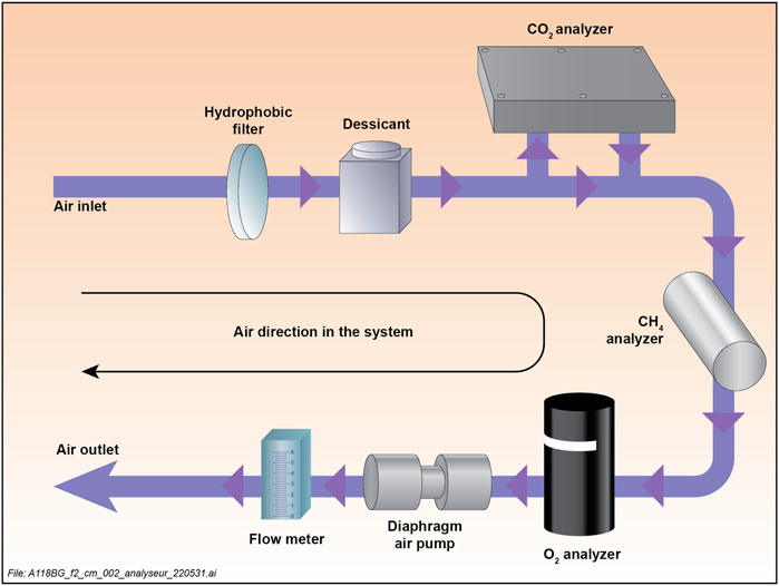
FIGURE 1. Conceptual diagram and components of the SAGES system.
2.2 Plexiglass equilibration system (PES)
The Plexiglass Equilibration System (PES) was designed to continuously generate a dynamic headspace for gas measurement from turbine water inside the generating station without external intervention and with minimal maintenance in mind. It is a flow through system that combines characteristics of the Weiss-type and bubble-type equilibrators (Gulzow et al., 2011; Webbs et al., 2016; Yoon et al., 2016). Like most equilibrators, it aims to enhance gas exchanges between the water sample in the equilibration chamber and a close recirculating air loop sets between the gas analyser and the headspace. While the Spray-type equilibrator use a nozzle to disperse micro droplets of water into the headspace and the marble-type equilibrators enhanced the exchange rate by increasing water-air contact area through marbles, the PES rely on an air-stone to generate a constant flow of gas microbubbles that circulate through the water sample.
The system is composed of two interconnected 6-mm thick plexiglass compartments (Figure 2). Water enters the system through the air-tight inner compartment and flows to the outer compartment through a communicating groove at the bottom. The outer compartment has a water spill out groove at the top. When the system is operating, water enters and simultaneously fills both containers until it reaches the top groove of the outer compartment. It then flows out into a drain, thereby stabilizing the water level in the equilibrator and creating a membrane-free water-capped dynamic headspace at the top of the inner compartment. A bleed port with 2-m long tubing allows for pressure equilibration during initial filling and during measurement. A gas ports on the top of the inner compartment allow air to be sampled from the headspace using the SAGES built-in air pump set to 2 LPM. The pump continuously circulates the gas from the PES to the analyzer system and sends it back to the PES through the air stone installed at the bottom of the inner compartment. The air that exits the air stone, returns to the headspace has a constant flow of bubbles floating up through the water column. This pump-driven flow enables membrane-free equilibration to occur along with continuous gas sampling by the analyzer (Figure 2).
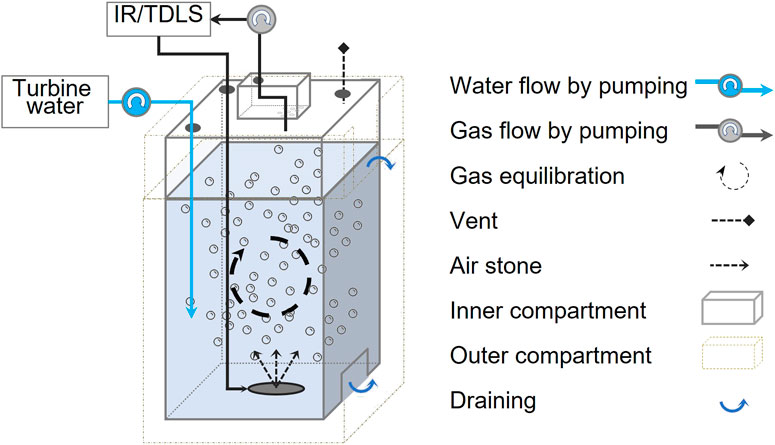
FIGURE 2. Conceptual diagram of the Plexiglas Equilibration System (PES). Schematization inspired by Yoon et al. (2016).
3 Methods
3.1 Instrument calibration
Each instrument was calibrated using reference gas covering the expected analytical range of the Québec (Canada) reservoir to be studied (Demarty et al., 2019). A standardized method was developed for all SAGES based on individual sensor requirements. The CO2 sensor was calibrated using three partial pressures (0, 1,000, and 5,000 ppm). Zero calibration was obtained using a CO2 gas stripper cartridge filled with fresh soda lime carbon dioxide absorbent. After each calibration, the sensor output was validated with the standard gas partial pressures of 0, 400, 1,000 and 5,000 ppm.
The CH4 sensor was calibrated and validated with 1.8 ppm and 100 ppm as reference gas values. The methane laser was also exposed to a reference gas PP of 10,000 ppm to collect information on the linearity at a high value, although it was not used to calibrate the sensor. Historical data from previous SAGES calibrations was analysed to complete the data set when required.
SAGES was compared to the Los Gatos Research Ultraportable Greenhouse Gas Analyzer (LGR UGGA) both in the laboratory and in the hydropower facility. The LGR UGGA was calibrated according to the instrument manual using gas PPs of 1,000 and 100 ppm of CO2 and CH4, respectively. The LGR UGGA calibration was validated using all available reference gas PPs for CO2 (400, 1,000 and 5,000 ppm) and CH4 (1.8 and 100 ppm) including a spot check at 10,000 ppm.
3.2 Analyzer comparison
A series of tests was conducted in the laboratory to compare SAGES performance with an LGR UGGA using side-by-side measurements of GHGs with ambient air, calibration gases and gases from the PES headspace. This was achieved by connecting the LGR UGGA to the SAGES main air loop with a gas manifold just prior to the gases entering the SAGES inlet port. The LGR UGGA was run in closed-loop configuration, and it recirculated the sample from the SAGES main loop using its built-in pump. Depending on the configuration, the SAGES air loop was connected directly to the PES headspace (closed loop), calibration gases or to an ambient air sample (open loop). All connections were made with 6.23-mm Bev-A-Line tubing.
Long-term unattended instrument comparison was conducted by installing a SAGES and an LGR UGGA in a Hydro-Québec facility between July 1 and 30 September 2020. SAGES drove the main PES air-loop/air-stone circuit as previously described and, because the LGR UGGA built-in pump could not drive the PES air-loop/air-stone, it was connected to the SAGES main air loop for the entire monitoring. Each measurement taken by the LGR UGGA (1 Hz) was transferred to the SAGES data logger using serial communication and recorded internally just like other sensor reading.
3.3 Equilibrators comparison
A series of tests was conducted to compare the PES performance to a commercially available device: a gas contactor (3M Liqui-Cel MM Series Membrane Contactor, length 222 mm). Each system was exposed to water samples of various gas concentrations generated by injecting reference gases (CO2 and CH4) in a 200-L water tank. A PES was connected to a SAGES as previously described, while a second SAGES was connected to the lumen side of the contactor in a closed recirculating loop. This configuration allowed the water to be simultaneously sampled and analyzed from the test tank using both equilibrators. Water was pumped to the contactor using a Solinst peristaltic pump set to 2.5 LPM and to the PES using a linear flow pump at a rate of 2.5 LPM. A total of 25 trials were conducted by injecting gases through an air stone installed at the bottom of the water tank to generate a partial pressure gradient of CO2 between 1,000 and 2,000 ppm, and of CH4 between 1.8 and 600 ppm. Following each injection, water was sampled from the pumps until the gases equilibrated in the PES and contactor. The analyzers were set to store the gas PP every second during the equilibration process. In such conditions, the equilibrated concentration was directly available, but to allow for a robust comparative method, gas PP versus time were fitted against a first order equilibration equation (describe in the Statistical analysis and curve fitting section). This enabled us to mathematically estimate gas PP in the headspace at equilibrium (PEQUI), but also to examine and compare the equilibration kinetic for each trial, gas and device.
3.4 Long term monitoring
Two systems were installed in cascading hydropower facilities between 1 January 2021, and 1 October 2021, to test how SAGES and the PES performed during prolonged unattended monitoring. Each SAGES was installed inside a generating station in a protective cabinet with direct access to turbinated water and set to store 15-min averages throughout the monitoring. The PES water inlet was connected directly to the generating station turbine to allow pump-free continuous access to turbine water for measurement. The water flow rate was set to 6 LPM by downregulating the turbine’s internal pressure to 20 PSI using a pressure regulator and the output flow was manually finetuned using a ball valve. SAGES was connected to the PES using 6.23-mm tubing and the gas sample was recirculated using the built-in diaphragm pump from the headspace to the instruments and back to the PES and air stone as previously described (see also Figure 2). Each system was powered with a 12-V power supply connected directly to the electrical outlet in the cabinet. Brief maintenance involving data collection, system integrity checks and PES cleaning was performed in the middle of the test, which took place in early spring (May).
3.5 Statistical analysis and curve fitting
To precisely determine the gas PP at equilibrium and associated error, the equilibration data obtained with the PES and contactor for each laboratory trial was modeled using the following first order equilibration equation (Eq. 1):
where Y is the gas partial pressure (pCO2, pCH4 or pO2) measured at time t in seconds, PEQUI is the gas partial pressure in the equilibrated headspace (targeted value), C0 is the gas partial pressure at the beginning of the equilibration phase and k is the equilibration rate coefficient.
To combine all the trials and compare the CO2/CH4 gas equilibration curve between the PES, the contactor and the different gas PP concentrations, the gas PP was normalized to PEQUI (0%–100%). The normalized data were fitted to the first order equilibration model (Eq. 1) and the fitted parameters were then used to calculate the equilibration time required to reach any fraction of PEQUI for CO2 or CH4 in the PES and contactor according to equation 2 (Eq. 2):
where Tn is the time in seconds required to reach n fraction of PEQUI and PEQUI, and C0 and k represent the parameters obtained using Eq. 1 for the corresponding first order equilibration model. All calculations, curve fitting and statistical analysis were conducted using Graphprism 5.0.
4 Results and discussion
4.1 SAGES analytical performance
The SAGES integrate commercially available probes, whom performances are detailed by the manufacturers. The objective here is to validate the accuracy of the whole system assembly (probes, tubing, dessicant, pump, and connectors) rather than individual probes and make sure it compared to expected manufacturer performances, match the expected measuring range but also to define the limits of the system. The accuracy and precision of SAGES was assessed by measuring reference gas PP under controlled conditions. When exposed to 400 ppm, 1,000 ppm and 5,000 ppm of CO2, SAGES records average values of 400.3 ppm (SD ± 0.7), 999.4 ppm (SD ± 1.2) and 4,998 ppm (SD ± 3.3), respectively (Figure 3). The maximum variation obtained, calculated as the difference between the minimum and maximum values, was 3.6 ppm for 400 ppm, 6.5 ppm for 1,000 ppm and 18 ppm for 5,000 ppm (see Supplementary Table S1). These variations corresponded to a maximum error of 0.5% on the full-scale range, which translates to an error of ±2 ppm in the worst-case scenario when measuring pCO2 under ambient air conditions.
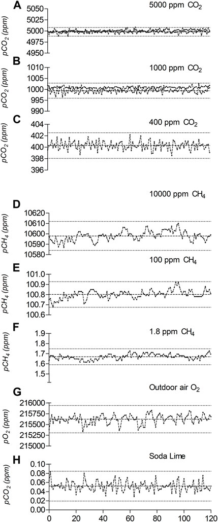
FIGURE 3. Gas PP and typical variability obtained with SAGES exposed to different gas concentrations from the reference tank (A–F), outdoor air (G) or the soda lime cartridge (H). Raw data, the average and error (3SD–worst scenario) are presented for each condition.
When exposed to 1.8 and 100 ppm of CH4, SAGES returned values averaging 1.67 (SD ± 0.03) and 100.8 ppm (SD ± 0.04). This corresponds to an error of less than 1% at 100 ppm CH4 and an underestimation of the CH4 PP of 7% in 1.8 ppm standard gas (Figure 3). According to the manufacturer, the CH4 laser is linear to at least 1,000 ppm of CH4. In the laboratory, the analyzer was exposed to concentrations of up to 10,000 ppm pCH4 and returned an average value of 10,451 ppm (SD ± 5), i.e., about 5% above the expected reference gas PP (Figure 3). When compared to historical calibration data collected for 15 SAGES systems exposed to a 10,000-ppm CH4 standard tank, the inter-SAGES measured values varied from 10,002 to 11,116 ppm, with an average of 10,598 ppm (SD ± 260, n = 27). This indicates that all units overestimated the tank reported concentration, by up to 11% in the worst case. As an external reference, the LGR UGGA was also exposed to 10,000 ppm of CH4 during the testing procedure, however, the methane signal became saturated at a stable but unusable value of 6,757 ppm (SD ± 17).
Aside from the tests done with calibrated gas tanks, experiments were conducted with ambient outdoor air (in Montréal, Canada). During these tests, the pO2 varied between 215,335 ppm and 215,827 ppm, with an average of 215,623 ppm (SD ± 106; Figure 3). The average pCO2 obtained with CO2-depleted air using a gas stripper cartridge was 0.05 ppm (SD ± 0.01). The data summarized in Figure 3 provide a realistic portrait of the typical variation that can be obtained when using SAGES for gas monitoring. The obtained measuring range exceed the observed range reported in boreal reservoir (Tremblay et al., 2005) which make the integrate system suitable for water turbine gas monitoring.
4.2 Instrument comparison in the laboratory
An important source of uncertainty in our knowledge of reservoir gas fluxes arises from the methods used to get the data (Zhao et al., 2015). When introducing a new sampler in the field, the challenge is to ensure the consistency of the results with the methods used previously. Hence, the SAGES was compared to an LGR UGGA, which relies on cavity ring-down spectroscopy (CRDS) —an accurate and precise technology measuring both CO2 and CH4 PP and used as reference against new sensors (Lee et al., 2022) and in studies on GHGs emissions from reservoirs (De Bonville et al., 2020; Soued and Prairie, 2020; Borges et al., 2023). Both instruments were configured to simultaneously measured gas PP from calibrated gas, ambient air or gas samples extracted from water using the PES module. A total of 45 comparatives measurements were taken with pCO2 between 400 and 5,000 ppm and pCH4 between 1.8 and 600 ppm. The results from both instruments strongly correlated for the whole partial pressure range tested for CO2 and CH4 (Figure 4). The slopes of the linear regression are not significantly different from 1 and indicate that within this measurement range, SAGES measurements corresponded to those obtained with the LGR UGGA.
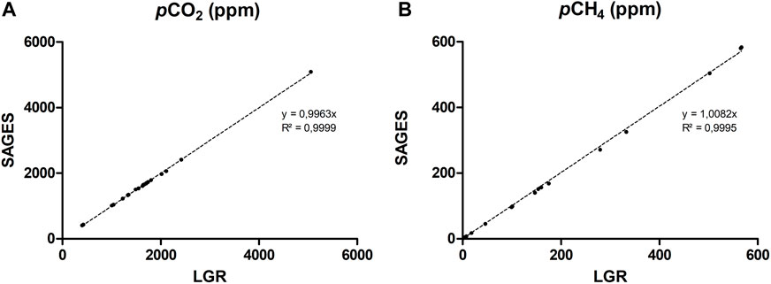
FIGURE 4. Comparison of gas PP (A) pCO2 and (B) pCH4 measured with an LGR UGGA (LGR) and SAGES, and the corresponding slope of the correlation between the instruments.
The average pCO2 measured by SAGES, for all conditions, was 1,601 ppm (SD ± 934.8), compared to 1,610 ppm (SD ± 933.1) with the LGR UGGA (Table 1). According to a paired t-test, these averages are marginally different (p = 0.04), with a mean of difference of 8.7 ppm. This difference corresponds to a 0.6-% deviation between the instruments when exposed to a range of 400 to 5,000 ppm of CO2. Similarly, the average pCH4 value measured by SAGES was 143.7 ppm (SD ± 191.7), whereas it was 144.2 ppm (SD ± 188.7) with the LGR UGGA (Table 1). The difference of only 0.5 ppm corresponds to a deviation of 0.4% between the instruments exposed to a range of 1.8–600 ppm of CH4. In this range, the averages were not statistically different when compared using a paired t-test (p = 0.71). For both gases, the differences between the instruments corresponded to less than 1 ppm over 100 ppm, (0.6% for pCO2 and 0.4%for pCH4).
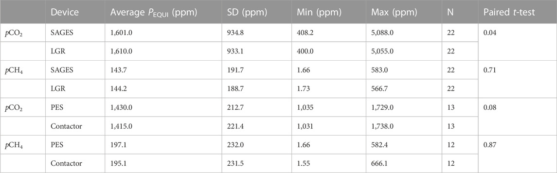
TABLE 1. Statistical PEQUI data [average, standard deviation, minimum, maximum, sample size (N) and paired t-test] for each gas (pCO2 and pCH4) obtained while comparing SAGES and the LGR UGGA (LGR) or the PES and contactor in the side-by-side trials.
When exposed to standard gas, the results showed that SAGES and the LGR UGGA measured an average that was similar for all concentrations (Supplementary Table S1) but the results obtained with the LGR UGGA provided a lower coefficient of variation, which is expected with CRDS instruments. This was observed for all tested conditions with both pCO2 and pCH4 values (Supplementary Table S1) and was particularly true for low pCH4 values. At 1.8 ppm, the difference was significant and the standard deviation of the LGR UGGA over 120 consecutively recorded measurements was 39 times lower (SD ± 0.0006) than the standard deviation obtained with SAGES (SD ± 0.026). Nevertheless, the average obtained from both instruments was not significantly different: 1.67 ppm for SAGES and 1.73 ppm for the UGGA.
The comparative results presented here demonstrate that the accuracy of SAGES matches that of a CRDS instrument (a reference in the field given the very stable data it returns). Under control conditions, there was no significant difference between the instruments with pCO2 readings between 400 and 5,000 ppm and pCH4 readings between 1.8 and 600 ppm. The LGR UGGA did however outperform SAGES with respect to data variability. In fact, SAGES standard deviation at a given partial pressure could be between 2 and 39 times higher than that obtained with the LGR UGGA. This difference could be observed for both CO2 and CH4 under most gas PP tested and was particularly pronounced when measuring low methane PP, i.e., close to ambient air conditions. Although higher than that of the LGR UGGA, the overall variability in SAGES measurements was low at less than 0.6% for pCO2 and 0.4% for pCH4 for any concentration in the full instrument range tested (Figure 3).
4.3 Instrument deployment on site
The SAGES was deployed in a generating station for 3 months. The test over a long time period in real sampling conditions was essential to validate the whole system robustness (working 24/24 h), sensor drift and PES unattended performance. Because there is no commercial solution to compared against, the SAGES was installed side by side to a LGR UGGA even if the latter is not a standalone solution and rely on the SAGES as described in Section 4.2. In these conditions, there was no significant differences between the instruments: the timeseries trends and partial pressure averages closely matched, the instruments did not significantly drift from each other, and the standard deviations of the data sets were identical at ±190 ppm for pCO2 and ±19 ppm for pCH4 (Figure 5).
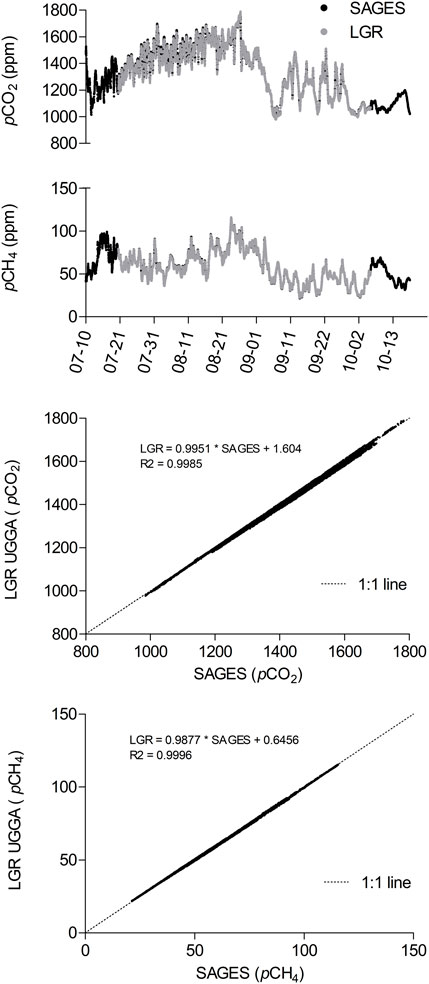
FIGURE 5. Comparison of gas PP measured over a three-month period with SAGES and an LGR UGGA (LGR) connected side by side in a generating station. Deviation from 1 to 1 line also presented.
During the three-month period, the average pCO2 and pCH4 values obtained with SAGES were 1,356 ppm (SD ± 190) and 57.7 ppm (SD ± 18.7), respectively, compared to 1,350 ppm (SD ± 189) and 56.6 ppm (SD ± 18.5) with the UGGA. During the period, the data was significantly correlated and was not different from a 1 to 1 line (Figure 5). It is worthy to note that the standard deviation values were similar for both instruments and represented the natural in situ variability with 14% for pCO2 and 33% for pCH4, well beyond individual bench performance values obtained in the laboratory with standard gases (below 1% variability, see previous section). To illustrate natural variability, let’s examine a few examples of studied ecosystems at different latitudes. For the young boreal Eastmain 1 reservoir, Demarty et al. (2011) reported mean summer water surface pCO2 decreasing from 2,205 ppm in 2006 to 1,126 ppm in 2008, with winter pCO2 reaching approx. 2,800 ppm below the ice cover. Concomitantly (2006–2008 period), the authors found that the average pCH4 varied from undetectable to approx. 1,000 ppm. At that time, profiles along the water column in a natural lake in the vicinity of the Eastmain 1 reservoir showed gas PP increasing from 700 to 3,000 ppm for CO2 and from 20 to 150 ppm for CH4. In a completely different ecosystem, the Pengxi River, which is the largest tributary of the Three Gorges Reservoir in China, Li et al. (2014) reported surface pCO2 ranging from approximately 26 to 4,087 ppm. Colas et al. (2020) have also reported long-term datasets from the equatorial reservoir Petit Saut in French Guyana and found surface pCO2 ranging from 235 to 5,860 ppm, and surface pCH4 ranging from 340 to 840 ppm, with an average pCH4 in deep water of 25,680 ppm. These data underline the fact that the attention given to the variability of an instrument should also depend on its uses. In real-life monitoring situations, the natural spatial and temporal pCO2 and pCH4 variability exceeded the bench variability and performance of both analyzers and therefore diminished the CRDS-associated benefits of the LGR UGGA when compared to SAGES simpler spectrophotometric technology.
4.4 Equilibrators comparison
Performance of the PES and membrane contactor to equilibrate CO2 and CH4 from water samples of various concentrations was assessed by measuring changes in the headspace gas concentration during individual equilibration trials. As seen in Figure 6, changes in CO2, CH4 and O2 concentrations followed a typical first order saturating exponential model for both equilibration devices (Kolb and Ettre, 2006). The equilibration process started with a pronounced change in the gas PP within the device headspace and gradually reached a steady-state equilibrium PEQUI corresponding to the gas PP in the water sample.
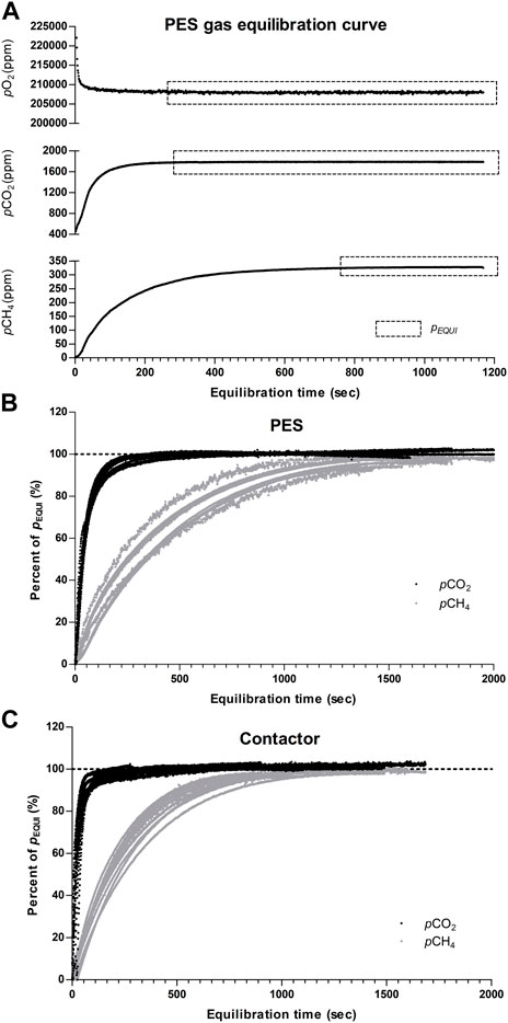
FIGURE 6. (A) Typical equilibration curve obtained within the PES headspace and steady-state equilibrium (PEQUI) for pO2, pCO2, and pCH4, normalized equilibration curve obtained for each trial with (B) The PES and (C) The commercial contactor.
Upon comparison, the PEQUI values calculated for each equilibration curve for both devices strongly correlate (Figure 7), despite their different designs (the PES is a membrane-free equilibrator, whereas the contactor relies on a hydrophobic semi-hollow microfiber tube). On average, the PEQUI values were 1,430 ppm of CO2 (SD ± 213) for the PES and 1,415 ppm of CO2 (SD ± 221) for the contactor (Table 1). This difference was not significant when compared using a paired t-test (p = 0.08); the mean difference was 15.7 ppm which represents a deviation of 1.1% between the equilibrators. For pCH4, the average PEQUI values were 197.1 ppm (SD ± 232.0) for the PES and 195.1 ppm (SD ± 231.5) for the contactor (Table 1). Again, the averages did not vary significantly when compared using a paired t-test; the mean difference was 2.0 ppm or a deviation of 1.0% between the devices.
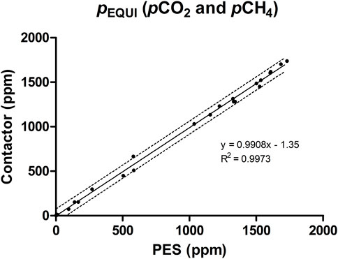
FIGURE 7. Comparison of PEQUI values obtained for pCO2 and pCH4 measurements from either the commercial contactor or the PES; correlation and 95% confidence interval also shown.
To compare both equilibration systems and evaluate their performance with specific gas and partial pressure values, data from individual trials were normalized to their respective PEQUI and combined (Figures 6B, C). Unsurprisingly, the analysis of the normalized data showed that all 24 trials followed the equilibration kinetic previously described. The data also showed that pCH4 required more time to reach PEQUI, and that its equilibration kinetic tended to be more heterogenous than that of pCO2 for both the PES and contactor. This heterogeneity can be explained by the difference in the initial gas PP: when the initial pCH4 was higher, the headspace partial pressure reached equilibrium faster and the curve tended to deviate from the average (Figures 6B, C). This effect was also true for pCO2 equilibration, but it was less visible in the dataset. Because of the properties of the equilibration kinetic, initial gas offset did not modify the partial pressure obtained at equilibrium PEQUI but rather the time required to reach the steady state.
The gas transfer curve model can be used to calculate the time required to reach PEQUI for the normalized data set and for individual trials (Table 2). All conditions combined, the time required to reach 95% of PEQUI was shorter for pCO2 (1.1–2.7 min) that for pCH4 (12.6–20.9 min). The contactor was 1.2 min faster to equilibrate CO2 and 8.7 min faster to equilibrate CH4 than the PES (Table 2). Regardless of the devices, the equilibration times correspond to data from previous studies reviewed in Webbs et al. (2016) and Yoon et al. (2016). The lower solubility of CH4 relative to CO2 explains why the latter reach steady state faster in both the contactor and PES. The longer equilibration time required by the PES can partly be explained by the low water flow rate in the PES during the experiments. In the laboratory trials reported in this paper, water could only be renewed at a rate of 2.5 LPM. These conditions were optimal for the contactor, which is designed for low flow rates and has a residence time (Tw) below 2 s. For the PES, it resulted in a Tw of 212 s. During typical deployment in generating stations, however, the PES working flow rate is 6–8 LPM, which corresponds to a Tw of 88 s, which would likely result in a faster equilibration time. Another difference is associated with the PES headspace design: while the contactor aims to maximize the exchange surface between air and water using microtubes, one of the PES design’s objectives is to avoid clogging by organic matter and sand so that the instrument can run without interruption. As with the contactor, the idea was to maximise the water to air volume ratio to shorten the equilibration time (Webbs et al., 2016) but, to prevent water from entering the analyzer air loop, the PES headspace had to be significantly larger and with an air volume of 1.1 L and thus require more time to reach steady state. This was an acceptable trade-off to allowed for uninterrupted measurement with potentially turbid and sandy water. In long-term monitoring, the gas PP are not expected to change rapidly and once the PES headspace reached equilibrium, the PP dynamically changed with the continuously-renewing water supply.
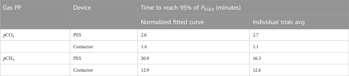
TABLE 2. Comparison of the time required to reach 95% of PEQUI when equilibrating pCO2 and pCH4 with the PES and contactor. Both results obtained from the single fit on the normalized data set and the averages of individual trials are shown.
4.5 Long-term monitoring in a generating station
In January 2023, eight SAGES were in action in Hydro-Quebec generating stations for 6 months or more. The entire dataset is not yet available; however a subset is presented on Figure 8, that presents a 10-month monitoring period in cascading generating stations (approximate distance of 70 km between the two stations) of the Romaine complex. The deployment of the two SAGES enabled more than 28,000 data points to be collected over the four local seasons, which is exceptional in boreal aquatic ecosystems where winter deployment or field campaigns are technically challenging. In the present article, the purpose was not to go in details with the time series analysis, but still, it is interesting to highlight the main trends observed. Both reservoirs (Romaine-2 upstream and Romaine-1 downstream) behaved similarly over time. The reservoir temperature at the water intake depth was around 4°C in winter and started to rise during spring freshet to reach its maximum in late August. From January to March, the pCO2 and pCH4 in the water column tended to be lower and more stable in both reservoirs. Water from the upstream reservoir also reached a maximum pO2 at the end of this period. The pCO2 and pCH4 values increase in April and early May, when it is customary for early spring changes to be observed: water mixing, ice melting, reservoir level changes and reservoir uses. In summer, pCO2 and pCH4 were higher and more variable with some pronounced variations. At this period discrepancies in CO2 and CH4 ranges appeared between the studied reservoirs; a more detailed study with ancillary information, would be necessary to possibly explain this phenomenon. During the entire monitoring period, the average pCO2 in the water turbinated from the upstream reservoir was 1,163 ppm (SD ± 252) while it was 1,368 ppm (SD ± 232) in the water turbinated in the downstream facility. The average pCH4 was 25.9 ppm (SD ± 23.2) in the upstream reservoir and 13.6 ppm (SD ± 8.6) in the downstream reservoir.
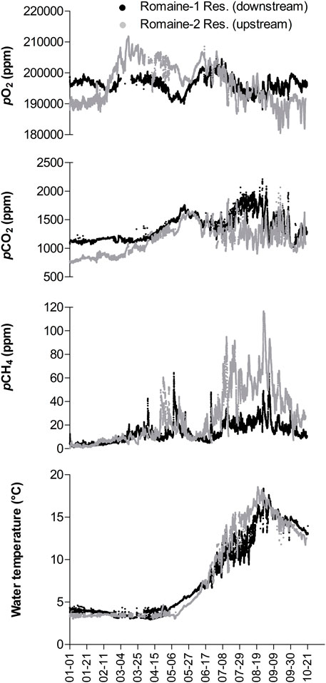
FIGURE 8. Ten-month time series of pO2, pCO2, pCH4, and water temperature (°C) readings obtained with a SAGES-PES system installed in Romaine-1 (downstream) and Romaine-2 (upstream) generating stations.
This long-term monitoring, and deployments made in other generating stations (data not shown) permitted to highlight strengths and weaknesses of the system in its targeted running environment. First, the SAGES readings did not drift. The pump used generally accumulated 10,000 h of running and were changed preventively; they did not represent a weakness to care of. Second, the PES was shown to be a good working solution. During the 10-month testing only two maintenance procedures were performed and the system remained fully operational. In former surveys made with the first automated system design (Demarty et al., 2009), the use of a membrane contactor for the same period of deployment required around 8 maintenances for the same period of deployment. Thanks to the design of the PES, water did not reach the SAGES and there was a continuous flow of gas bubbles within the PES air stone. This was a significant improvement over the contactor system that would have inevitably clogged with sand and organic matter in just a few days of continuous uses in the same water quality conditions. In the encountered conditions, a maintenance every 3–4 months was enough to ensure a proper use of the gas equilibrator and maintained a non-significant biofouling accumulation in the chamber. Water never stagnates in the system and there was noi difference in the reading just before and after every cleaning of the PES. The main source of error during the deployment comes from turbine stopped for maintenance or when power was not required. In those case, water was stagnant in the turbine chamber but still produce a flow in the PES and realist data in the SAGES. This can be easily overcome by processing the data only when the turbine is actively generating energy. The person in charge of the data management must have access to the turbinated flow time series to avoid misinterpretation of the results. Finally, the advantage of the Campbell data logger in allowing flexible and rapid programming of QAQC procedures permitted to output custom dataset easy to check and quickening maintenance.
The perspective of use of the SAGES in other environments are numerous. The detailed time series obtained can allow a fine analysis of the biogeochemical cycles in various ecosystems, even more if ancillary measurements are integrated to the study. As an example, Taillardat et al. (2022) deployed a SAGES for 2 months in a Canadian peatland and analysed time series measurements of rainfall, peatland water table depth, pCO2, pCH4 and dissolved oxygen at the outlet of a stream to study the carbon budget of the peatland. Alternatively, given the ready-to-use skills of the SAGES and the predictive ability of Eq. 1, a combination of SAGES and membrane contactor was used during ice-free period field campaigns on lakes and reservoirs to survey wide areas and numerous sampling sites (Demarty et al., 2020; Demarty et al., 2021). The SAGES being relatively cost effective compared to CRDS technology, it was possible to have two systems in parallel on the field and to sample simultaneously the epilimnion and the hypolimnion, hence reducing the time devoted to each station.
5 Conclusion
The system described in the current study provides a reliable plug and run tool for monitoring dissolve CO2 and CH4 in turbinated waters. The SAGES was proven to be accurate and stable both in the laboratory and throughout the different monitoring conditions, as shown with direct comparisons to alternative cutting-edge technologies. SAGES and PES can be installed in less than a day and the major advantage of the system is its autonomy: it provides year-round measurements in a safe manner. The normal wear of parts and the biofouling in the PES are the limiting factors for deployments longer than 4 months or for warmer water and close communication is necessary between generating station manager and data analyst to avoid misleading interpretation of the results in case of turbine interruption. Combining the time series gathered with discharge rates can undoubtedly furnish a trustworthy estimate of the degassing emissions related to hydropower production in any environment.
Data availability statement
The original contributions presented in the study are included in the article/Supplementary Material, further inquiries can be directed to the corresponding author.
Author contributions
CD: conceptualization, instrumental design, formal analysis, methodology, validation, writing—original draft and editing. MD: conceptualization, methodology, validation and editing. FB and AT: writing-review. All authors contributed to the article and approved the submitted version.
Funding
The authors would like to thank Hydro-Québec for funding the development and testing of the SAGES and PES.
Conflict of interest
CD and MD were employed by the company Aqua-Consult (Montreal, QC, Canada). FB and AT were employed by the company Hydro-Québec (Montreal, QC, Canada).
Supplementary material
The Supplementary Material for this article can be found online at: https://www.frontiersin.org/articles/10.3389/fenvs.2023.1194994/full#supplementary-material
References
Atamanktchuk, D., Tengberg, A., Thomas, P. J., Hovdenes, J., Apostolidis, A., Huber, C., et al. (2014). Performance of a lifetime-based optode for measuring partial pressure of carbon dioxide in natural waters. Limnol. Oceanogr.-Meth. 12, 63–73. doi:10.4319/lom.2014.12.63
Borges, A. V., Okello, W., Bouillon, S., Deirmendjian, L., Nankabirwa, A., Nabafu, E., et al. (2023). Spatial and temporal variations of dissolved CO2, CH4 and N2O in lakes edward and george (east africa). J. Gt. Lakes. Res. 49, 229–245. doi:10.1016/j.jglr.2022.11.010
Colas, F., Chanudet, V., Daufresne, M., Buchet, L., Vigouroux, R., Bonnet, A., et al. (2020). Spatial and temporal variability of diffusive CO2 and CH4 fluxes from the Amazonian reservoir Petit-Saut (French Guiana) reveals the importance of allochthonous inputs for long-term C emissions. Glob. Biogeochem. Cy. 34, e2020GB006602. doi:10.1029/2020GB006602
Cole, J., Prairie, Y., Caraco, N. F., McDowell, W., Tranvik, L., Striegl, R., et al. (2007). Plumbing the global carbon cycle: integrating inland waters into the terrestrial carbon budget. Ecosystems 10 (1), 171–184.
De Bonville, J., Amyot, M., Del Giorgio, P., Tremblay, A., Bilodeau, F., Ponton, D., et al. (2020). Mobilization and transformation of mercury across a dammed boreal river are linked to carbon processing and hydrology. Water Resour. Res. 56, 10. doi:10.1029/2020WR027951
DelSontro, T., Beaulieu, J. J., and Downing, J. A. (2018). Greenhouse gas emissions from lakes and impoundments: Upscaling in the face of global change. Limnol. Oceanogr.-Let. 3 (3), 64–75. doi:10.1002/lol2.10073
Demarty, M., Bastien, J., and Tremblay, A. (2011). Annual follow-up of gross diffusive carbon dioxide and methane emissions from a boreal reservoir and two nearby lakes in Québec, Canada. Biogeosciences 8, 41–53. doi:10.5194/BG-8-41-2011
Demarty, M., Bastien, J., Tremblay, A., Hesslein, R., and Gill, R. (2009). Greenhouse gas emissions from boreal reservoirs in Manitoba and Québec, Canada, measured with automated systems. Environ. Sci. Technol. 43, 8908–8915. doi:10.1021/es8035658
Demarty, M., Deblois, C., Bilodeau, F., and Tremblay, A. (2019). in Greenhouse gas emissions from newly-created boreal hydroelectric reservoirs of La Romaine complex in Québec, Canada - proceedings of the ICOLD Annual Meeting Editors J-P. Tournier, T. Bennett, and J. Bibeau (London: CRC Press).
Demarty, M., Deblois, C., Bilodeau, F., and Tremblay, A. (2020). Aménagements hydroélectriques de la Romaine-1, de la Romaine-2 et de la Romaine-3 – mesure des émissions de gaz à effet de serre des réservoirs par systèmes automatisés – Résultats 2015-2019. Report for Hydro-Québec Direction Environnement, 45.
Demarty, M., Deblois, C., Bilodeau, F., and Tremblay, A. (2021). Complexe de la Romaine – Étude des émissions de gaz à effet de serre des réservoirs de la Romaine 1, de la Romaine 2, de la Romaine 3 et de la Romaine 4 – Résultats 2020. Executive summary produced by Aqua-Consult. Direction Environnement: Englobe Corp. et Hydro-Québec, 22.
Demarty, M., and Tremblay, A. (2017). Long term follow-up of pCO2, pCH4 and emissions from Eastmain 1 boreal reservoir, and the Rupert diversion bays. Can. Ecohydrol. Hydrobiol. 19 (4), 529–540. doi:10.1016/j.ecohyd.2017.09.001
International Panel on Climate Change (IPCC). (2019). Wetlands, pp 7.2-7.52. In E. Calvo Buendia, K. Tanabe, A. Kranjc, J. Baasansuren, M. Fukuda, S. Ngarizeet al. Refinement to the 2006 IPCC guidelines for national greenhouse gas inventories – volume 4 agriculture, forestry and other land use. Geneva, Switzerland: IPCC.
Grilli, R., Birot, D., Schumacher, M., Paris, J-D., Blouzon, C., Donval, J-P., et al. (2021). Inter-comparison of the spatial distribution of methane in the water column from seafloor emissions at two sites in the Western black sea using a multi-technique approach. Front. Earth Sci. 9, 626372. doi:10.3389/feart.2021.626372
Gülzow, W., Rehder, G., Schneider, B., Schneider, J., Deimling, V., and Sadkowiak, B. (2011). A new method for continuous measurement of methane and carbon dioxide in surface waters using off-axis integrated cavity output spectroscopy (ICOS): An example from the Baltic Sea. Limnol. Oceanogr.-Meth. 9, 176–184. doi:10.4319/lom.2011.9.176
Gülzow, W., Rehder, G., Schneider, B., Schneider, V., Deimling, J., Seifert, T., et al. (2013). One year of continuous measurements constraining methane emissions from the Baltic Sea to the atmosphere using a ship of opportunity. Biogeosciences 10, 81–99. doi:10.5194/bg-10-81-2013
Johnson, J. E. (1999). Evaluation of a seawater equilibrator for shipboard analysis of dissolved oceanic trace gases. Anal. Chim. Acta 395, 119–132. doi:10.1016/S0003-2670(99)00361-X
Kemenes, A., Forsberg, B. R., and Melack, J. M. (2007). Methane release below a tropical hydroelectric dam. Geophys. Res. Lett. 34, L12809. doi:10.1029/2007GL029479
Kolb, B., and Ettre, L. S. (2006). “Theoretical background of HS-GC and its applications,” in Static headspace-gas chromatography Editors B. Kolb, and L. S. Ettre (New Jersey: Wiley Hoboken), p19–p50.
Koschorreck, M., Prairie, Y., Kim, J., and Marcé, R. (2021). Technical note: CO2 is not like CH4 - limits of and corrections to the headspace method to analyse pCO2 in fresh water. Biogeosciences 18, 1619–1627. doi:10.5194/bg-18-1619-2021
Lee, D. J. J., Kek, K. T., Wong, W. W., Nadzir, M. S. M., Yan, J., Zhan, L., et al. (2022). Design and optimization of wireless in-situ sensor coupled with gas–water equilibrators for continuous pCO2 measurement in aquatic environments. Limnol. Oceanogr.-Meth. 20 (8), 500–513. doi:10.1002/lom3.10500
Levasseur, A., Mercier-Blais, S., Prairie, Y. T., Tremblay, A., and Turpin, C. (2021). Improving the accuracy of electricity carbon footprint: Estimation of hydroelectric reservoir greenhouse gas emissions. Renew. Sust. Energy Rev. 136, 110433. doi:10.1016/j.rser.2020.110433
Li, Z., Zhang, Z., Xiao, Y., Guo, J-S., Wu, S., and Jing, L. (2014). Spatio-temporal variations of carbon dioxide and its gross emission regulated by artificial operation in a typical hydropower reservoir in China. Environ. Monit. Assess. 186, 3023–3039. doi:10.1007/s10661-013-3598-0
Loken, L. C., Crawford, J. T., Schramm, P. J., Stadler, P., Desai, A. R., and Stanley, E. H. (2019). Large spatial and temporal variability of carbon dioxide and methane in a eutrophic lake. J. Geophys. Res. Biogeosciences 124, 2248–2266. doi:10.1029/2019JG005186
Nakayama, T., and Pelletier, G. (2018). Impact of global major reservoirs on carbon cycle changes by using an advanced eco-hydrologic and biogeochemical coupling model. Ecol. Model. 387, 172–186. doi:10.1016/j.ecolmodel.2018.09.007
Peeters, F., Atamanchuk, D., Tengberg, A., Encinas-Fernandez, J., and Hofmannet, H. (2016). Lake metabolism: Comparison of lake metabolic rates estimated from a diel CO2 and the common diel O2-technique. PLoS ONE 11 (12), e0168393. doi:10.1371/journal.pone.0168393
Prairie, Y. T., Alm, J., Beaulieu, J., Barros, N., Battin, T., Cole, J., et al. (2017). Greenhouse gas emissions from freshwater reservoirs: What does the atmosphere see? Ecosystems 21, 1058–1071. doi:10.1007/s10021-017-0198-9
Prairie, Y. T., Mercier Blais, S., Harrison, J. A., Soued, C., del Giorgio, P. A., Harby, A., et al. (2021). A new modelling framework to assess biogenic GHG emissions from reservoirs: The G-res tool. Environ. Modell. Softw. 143, 105117. doi:10.1016/j.envsoft.2021.105117
Raymond, P., Hartmann, J., Lauerwald, R., Sobek, S., McDonald, C., Hoover, M., et al. (2013). Global carbon dioxide emissions from inland waters. Nature 503, 355–359. doi:10.1038/nature12760
Scherer, L., and Pfister, S. (2016). Hydropower’s biogenic carbon footprint. PLoS ONE 11 (9), e0161947. doi:10.1371/journal.pone.0161947
Sepulveda-Jauregui, A., Martinez-Cruz, K., Strohm, A., Walter Anthony, K. M., and Thalasso, F. (2012). A new method for field measurement of dissolved methane in water using infrared tunable diode laser absorption spectroscopy. Limnol. Oceanogr.-Meth. 10, 560–567. doi:10.4319/lom.2012.10.560
Soued, C., and Prairie, Y. T. (2020). The carbon footprint of a Malaysian tropical reservoir: Measured versus modelled estimates highlight the underestimated key role of downstream processes. Biogeosciences 17, 515–527. doi:10.5194/bg-17-515-2020
Staudinger, C., Strobl, M., Fischer, J. P., Thar, R., Mayr, T., Aigner, D., et al. (2018). A versatile optode system for oxygen, carbon dioxide, and pH measurements in seawater with integrated battery and logger. Limnol. Oceanogr.-Meth. 16, 459–473. doi:10.1002/lom3.10260
Taillardat, P., Bodmer, P., Deblois, C. P., Ponçot, A., Prijac, A., Riahi, K., et al. (2022). Carbon dioxide and methane dynamics in a peatland headwater stream: Origins, processes and implications. JGR Biogesciences. 127, e2022JG006855. doi:10.1029/2022JG006855
Teodoru, C. R., Bastien, J., Bonneville, M.-C., del Giorgio, P. A., Demarty, M., Garneau, M., et al. (2012). The net carbon footprint of a newly created boreal hydroelectric reservoir. Glob. Biogeochem. Cy. 26, GB2016. doi:10.1029/2011GB004187
Tremblay, A., Therrien, J., Hamelin, B., Wichmann, E., and LeDrew, L.J. (2005). “GHG emissions from boreal reservoirs and natural aquatic ecosystems,” in Greenhouse Gas Emissions: Fluxes and Processes, Hydroelectric Reservoirs and Natural Environments. Editors A. Tremblay, L. Varfalvy, C. Roehm, and M. Garneau (Berlin, Heidelberg: New York: Springer-Verlag), 209–231.
Wang, W., Roulet, N. T., Kim, Y., Strachan, I. B., del Giorgio, P. A., Prairie, Y. T., et al. (2018). Modelling CO2 emissions from water surface of a boreal hydroelectric reservoir. Sci. Total Environ. 612, 392–404. doi:10.1016/j.scitotenv.2017.08.203
Webbs, J. R., Maher, D. T., and Santos, I. R. (2016). Automated, in situ measurements of dissolved CO2, CH4, and d13C values using cavity enhanced laser absorption spectrometry: Comparing response times of air-water equilibrators. Limnol. Oceanogr.-Meth. 14, 323–337. doi:10.1002/lom3.10092
Weiss, R. F. (1974). Carbon dioxide in water and seawater: The solubility of a non-ideal gas. Mar. Chem. 2, 203–215. doi:10.1016/0304-4203(74)90015-2
Xiao, S., Liu, L., Wang, W., Lorke, A., Woodhouse, J., Grossart, H.-P., et al. (2020). A Fast-Response Automated Gas Equilibrator (FaRAGE) for continuous in situ measurement of CH4 and CO2 dissolved in water. Hydrol. Earth Syst. Sci. 24, 3871–3880. doi:10.5194/hess-24-3871-2020
Keywords: degassing, hydropower, reservoirs, instrumentation, long-term monitoring, CO2 and CH4 concentration
Citation: Deblois CP, Demarty M, Bilodeau F and Tremblay A (2023) Automated CO2 and CH4 monitoring system for continuous estimation of degassing related to hydropower. Front. Environ. Sci. 11:1194994. doi: 10.3389/fenvs.2023.1194994
Received: 27 March 2023; Accepted: 08 June 2023;
Published: 16 June 2023.
Edited by:
Shaoda Liu, Beijing Normal University, ChinaReviewed by:
Ji-Hyung Park, Ewha Womans University, Republic of KoreaLongfei Yu, Tsinghua University, China
Copyright © 2023 Deblois, Demarty, Bilodeau and Tremblay. This is an open-access article distributed under the terms of the Creative Commons Attribution License (CC BY). The use, distribution or reproduction in other forums is permitted, provided the original author(s) and the copyright owner(s) are credited and that the original publication in this journal is cited, in accordance with accepted academic practice. No use, distribution or reproduction is permitted which does not comply with these terms.
*Correspondence: C. P. Deblois, Y2hhcmxlcy5kZWJsb2lzQGFxdWFjb25zdWx0LmNh
†These authors have contributed equally to this work and share last authorship