Groundwater monitoring and specific yield estimation using time-lapse electrical resistivity imaging and machine learning

This paper presents an alternative method for monitoring groundwater levels and estimating specific yields of an unconfined aquifer under different seasonal conditions. The approach employs the Time-Lapse Electrical Resistivity Imaging (TL-ERI) method and machine learning-based time series clustering. A TL-ERI survey was conducted at ten sites (WS01-WS10 sites) throughout the dry and wet seasons, with five-time measurements collected for each site, in the Taichung-Nantou Basin along the Wu River, Central Taiwan. The obtained resistivity raw data was inverted and converted into normalized water content values using Archie’s law, followed by applying the Van Genuchten (VG) model for the Soil Water Characteristic Curve to estimate the Groundwater Level (GWL), and estimated the theoretical specific yield (S_y) by computing the difference between the saturated and residual water contents of the fitted VG model. In addition, the specific yield capacity (S_c), representing the nature of the storage capacity in the aquifer, was also calculated. The results showed that this approach was able to estimate those hydrogeological parameters. The spatial distribution of the GWL reveals that during the dry-wet seasons from February to July, there was a high GWL that extended from southeast to northwest. Conversely, during the wet-dry seasons from July to October, the high GWL shrank, which can be attributed to recharge variations from rainfall events. The determined spatial distribution of S_y and S_c fall within the range of 0.03–0.24 and 0.14–0.25, respectively. To quantitatively establish areas of similar groundwater level changes along with the VG model parameter variations during the study period, a Time series Clustering analysis (TSC) was performed by utilizing Hierarchical Agglomerative Clustering (HAC). The findings suggest that the WS03 site is a promising area for further investigation due to its highest S_c value with a slight change in groundwater levels during the dry and wet seasons. This study brings an advanced development of the geoelectrical method to estimate regional hydrogeological parameters in an area with limited available groundwater observation wells, in different seasonal conditions for groundwater management purposes.

1 Introduction

Monitoring and evaluating regional hydrogeological parameters, including groundwater levels and specific yield over time, is essential for understanding the impact of climate change on groundwater systems. Traditionally, these parameters are acquired from observation wells alongside pumping wells (Ramsahoye and Lang, 1961; Taylor and Alley, 2001; Gopinathan et al., 2020). However, these approaches can be challenging, especially in regions with few or no available observation and pumping wells, as it can be expensive to install and maintain them. To address this issue, this study aims to develop an alternative method to monitor groundwater levels and estimate specific yields by applying Time-Lapse Electrical Resistivity Imaging (TL-ERI). TL-ERI offers numerous benefits that make it a valuable method for monitoring groundwater. Firstly, it is non-invasive and non-destructive, minimizing its adverse effects on the environment. Secondly, it provides high spatial coverage through the utilization of multi-channel electrodes. Thirdly, TL-ERI enables continuous monitoring, facilitating the assessment of groundwater levels and variations over extended periods. Moreover, TL-ERI presents a cost-effective alternative to traditional observation wells. Additionally, TL-ERI exhibits versatility in various hydrogeological settings, making it adaptable to diverse research and monitoring objectives. Finally, it demonstrates high sensitivity to changes in water content (Lech et al., 2020; Wahab et al., 2021). Owing to these advantages, several previous works utilized this method. For instance, Tesfaldet and Puttiwongrak (2019) used time-lapse electrical resistivity to characterize the seasonal groundwater recharge through the vadose zone and stream, and their result showed a significant decrease in resistivity in the transition of the dry season to the rainy season and vice versa. Aduojo et al. (2018) investigated the impact of seasonal variation on groundwater quality around the dumpsite using the time-dependent electrical resistivity method. Chang et al. (2016) conducted a time-lapse resistivity method during a pumping test. Through the study, they found that the variation in the resistivity changes in the vadose zone correlated to the change in groundwater level in the stepwise phase, which means that the measured vertical resistivity changes can indicate the depths of groundwater tables. Moreover, Bai et al. (2021) integrated time-lapse electrical resistivity and self-potential data to monitor the groundwater flow in the vadose zone. In addition, many attempts have been made by researchers to extract more information about the hydrogeological parameters derived from the resistivity method, such as hydraulic conductivity, specific yield, and transmittivity (Chang et al., 2017; Dietrich et al., 2018; Perdomo et al., 2018; Hasan et al., 2020; Akhter et al., 2022). Although TL-ERI has shown promising results in groundwater studies, there are notable challenges associated with its implementation, including the equipment and logistical prerequisites, such as the number of electrodes and the involvement of field researchers, as well as limitations in the depth of penetration and the intricacy involved in interpreting the acquired data. To address these challenges, meticulous preparations for data acquisition, processing, and interpretation were undertaken in this study.

This study was conducted in the Taichung-Nantou Basin along the Wu River in Central Taiwan. Despite the annual precipitation exceeds 2.500 mm, which is 2.5 times the global average, only 18% of surface runoff can be utilized for domestic, agricultural, and industrial purposes. Geographical features as well as the uneven spatial and temporal distribution of rainfall, have contributed to this phenomenon (Hsu et al., 2020; Huang et al., 2012; Hwang, 2003; Lee et al., 2006; Wang et al., 2021). Moreover, Hsu et al. (2020) have already noted a significant disparity in the precipitation between the wet and dry seasons. Approximately 70% of rainfall occurs during the wet season, which spans from May to October and is characterized by seasonal monsoons and typhoons, whereas limited rainfall is observed in the dry season, from November to April. Consequently, Taiwan faces a relatively high risk of experiencing meteorological drought (Huang et al., 2012). Additionally, a study by Hung and Shih. (2019) indicated that the majority of drought cases occur during the dry season, particularly in central to southern Taiwan, which includes the present study area. If the meteorological drought persists for an extended period and affects the groundwater system, it can lead to groundwater drought, posing a significant problem in Taiwan, as groundwater serves as a major water resource for the country (Bai et al., 2019; Chen et al., 2020; Han et al., 2019; Yeh and Hsu, 2019). Thus, conducting a comprehensive analysis and evaluation of groundwater under different seasonal conditions is highly recommended to facilitate effective management practices in the study area.

The purpose of the present study is to introduce an innovative approach to groundwater monitoring and evaluation. This approach involves integrating in-situ resistivity surveys into soil-water characteristic models and utilizing the time series clustering algorithm, specifically Hierarchical Agglomerative Clustering, along with Principal Component Analysis (PCA) for result interpretation. The proposed method offers an alternative and efficient means for researchers to determine regional hydrogeological parameters, particularly in areas with limited available observation wells and under varying seasonal conditions. Moreover, this study demonstrates the application of machine learning techniques to analyze and interpret the dataset, highlighting its potential for groundwater management purposes.

2 Materials and methods

2.1 The study area

Taiwan is bisected by The Tropic of Cancer, where its northern and central regions are subtropical while the southern regions are tropical. This distinct condition leads the weather to vary considerably across the island (Chen et al., 2021; Dibaj et al., 2020; Hung et al., 2017). The accumulated precipitation in the study area during 2018 is shown in Figure 1. It fluctuated during the dry and wet seasons with the highest and the lowest accumulated precipitation in August and December with 449.5 mm (the wet season) and 2.0 mm (the dry season), respectively.

FIGURE 1

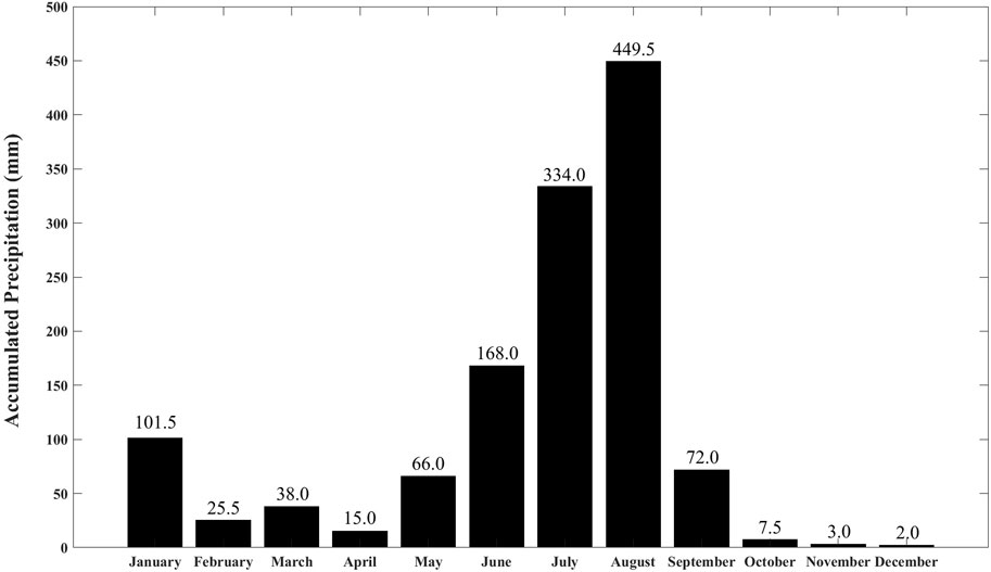
FIGURE 1. The annual precipitation accumulation in the study area during 2018.

The study area is located in the Taichung-Nantou Basin along the Wu River in Central Taiwan (Figure 2). This basin covers parts of Taichung city, Nantou County, and Changhua County. The study area encompasses the Maoluo River in the south, the Touke Hill lands of Nantou in the east, the southern district of Taichung City in the north, and the Bagua Plateau in the west. The average ground elevation ranges from 30 to 65 m above sea level, with the highest elevation found in the southeastern region and gradually decreasing towards the northwest of the study area.

FIGURE 2

FIGURE 2. The geographical map from the Taichung-Nantou Basin. The survey area (red rectangle) is located in between the Hills across the Wu River.

Furthermore, the geological setting of the study area is mostly composite by the alluvial deposits, in which the western side of the survey area faces Bagua Hill, which includes the Toukoshan formation and the terrace deposits, as well as the Pakushan Anticline. The Tokushan formation is classified into three divisions: the lower division (up to 900 m thick) consists of sandstone and shale with a pebbly horizon, the middle division (50–100 m) consists of an alternating bed of sand, clay, and gravel that containing fresh-water, the upper-division consists of several hundred meters of massive conglomerate with a few thin beds of crudely cross-bedded sandstone. The terrace deposits consist mainly of unconsolidated gravel with flat-lying sandy or silty lenses. The west side of the survey area is Touke Hill, where the Chelungpu Fault is found along the edge of the hill. The area is also traversed by two rivers, the Maoluo river and the Wu River, whose branches confluence on the northwest right. The alluvial deposits mainly consist of thick gravel and sand with good permeability, making the area highly potential for groundwater recharge (Ho and Chen, 2000).

2.2 The electrical resistivity imaging design and the resistivity survey

To investigate the groundwater condition, we conducted ten Electrical Resistivity Imaging (ERI) survey lines (shown in red in Figure 3) around three observation wells (shown as magenta circles). In order to analyze the influence of seasonal conditions on the trends of ERI results, we performed time-lapse surveys at consistent survey sites during both the dry and wet seasons. A comprehensive dataset spanning five distinct periods was collected, encompassing February (dry season), May (transition from dry to wet seasons), July (wet season), September (wet season), and October (transition from wet to dry seasons). This methodological approach enabled us to meticulously examine and analyze the discernible patterns exhibited by the ERI results across diverse seasonal contexts.

FIGURE 3

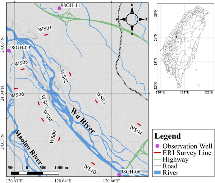
FIGURE 3. The distribution of resistivity survey lines (red line) along the Wu River. The magenta circle represents the location of the observation wells.

The fundamental idea of the resistivity method involves injecting current into the subsurface using a pair of electrodes. This current generates a potential difference in the subsurface, which is measured and monitored by another pair of electrodes, resulting in the measurement of the apparent resistivity. It’s important to note that the apparent resistivity represents the collective measurements of the electrical properties of all the subsurface layers within the corresponding electrode configuration. Therefore, an additional inversion process is required to determine the true resistivity value, which can provide valuable information about the subsurface lithology or materials. Figure 4 summarizes the workflow of the present study.

FIGURE 4

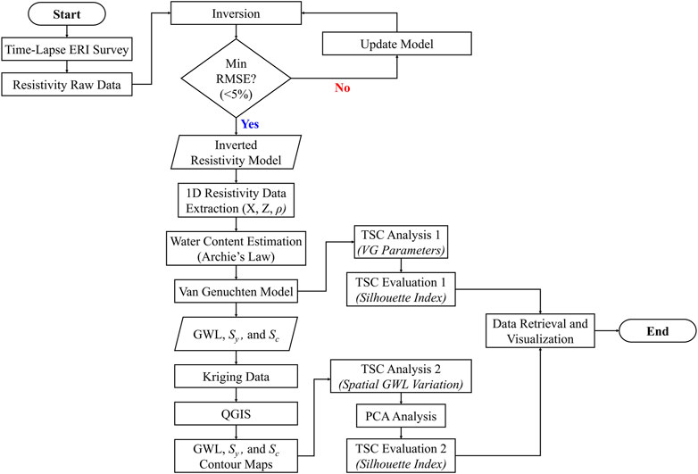
FIGURE 4. The workflow of the present study.

This study utilized the 4-point light 10 W resistivity meter and the active electrode (ActEle) system (Lippmann Geophysical Instruments) (Lippman, 2014) in Wenner-Schlumberger configuration with a 1 m electrode spacing for the field data measurements. Wenner-Schlumberger configuration is less susceptible to noise than the other arrays, which means that it yields a high signal-to-noise ratio with better sensitivity to horizontal structure (Dahlin and Zhou, 2004). The raw data was later inverted with the EarthImager2D™ version 2.4.2.627 (Advanced Geosciences, 2006). For a detailed review of the resistivity method inversion techniques, we forward readers to Sharma and Verma (2015).

2.3 Estimation of the groundwater level and the specific yield

After the inverted resistivity section was obtained, we carried out the groundwater level estimation of the study area. First, we calculated the water contents in the five vertical profiles in the central part of each resistivity survey line for the estimation of water content by adopting a similar process to Dietrich et al. (2018). We may deduce from Archie’s Law (Archie, 1942) how formation resistivity relates to porosity, saturation, and pore water resistivity in a clay-free matrix:

$\mathit{\rho }=\mathit{\alpha }{\mathit{\rho }}_{\mathit{w}}{\mathit{\varphi }}^{-\mathit{n}}{{\mathit{S}}_{\mathit{w}}}^{-\mathit{m}}(1)$

where $\rho$ is the formation resistivity, ${\rho }_w$ is the pore water resistivity, $\varphi$ is the porosity, $S_w$ is the saturation, and $\alpha ,$ m, and n are empirical parameters. Parameters m and n are usually termed saturation exponent and cementation factor, respectively. For general homogeneous rocks and soils, m ranges from 1.8 to 2.2, and n is about 2; so, m = n ≅ 2. On the other hand, it should be noted that the empirical factor $\alpha$ is not included in its original form of Archie’s law [Detailed in Glover. (2015)].

As it is known, the volumetric water content ($\theta$) at the saturation point is equivalent to the total soil pore space, expressed as

$\mathit{\theta }={\mathit{\varphi }}^{-\mathit{n}}{{\mathit{S}}_{\mathit{w}}}^{-\mathit{m}}(2)$

considering the value of m and n, and substituting Eq. 2 into Eq. 1, ${\rho }_f$ will yield

$\mathit{\rho }={\mathit{\rho }}_{\mathit{w}}{\mathit{\theta }}^{-\mathbf{2}}(3)$

If we assume that the resistivity value varies only with the water saturation, we can calculate the normalized relative saturation (S_r) at different depths in the vadose zone as

${\mathit{S}}_{\mathit{r}}=\frac{{\mathit{\theta }}_{\mathit{u}}}{{\mathit{\theta }}_{\mathit{s}}}=\sqrt{\frac{{\mathit{\rho }}_{\mathit{s}}}{{\mathit{\rho }}_{\mathit{u}}}}(4)$

where ${\theta }_u$, ${\theta }_s$, ${\rho }_u$, and ${\rho }_s$ are unsaturated layer volume water content, saturated layer volume water content, unsaturated layer formation resistivity, and saturated layer formation resistivity, respectively. In this case, the lowest resistivity value obtained from the ERI of each site was set as ${\rho }_s$, and the data of the topmost 2 m are eliminated because it represents the properties of the surface soil layer instead of the properties of the gravel layer. Next, we can obtain the normalized volumetric water content by multiplying $S_r$ and ${\varphi }_A$ (Average Porosity, 0.26), expressed as

$\mathit{\theta }={\mathit{S}}_{\mathit{r}}{\mathit{\varphi }}_{\mathit{A}}(5)$

Figure 5 depicts how the normalized volumetric water content varies from the ground surface to the saturated layer in an unconfined aquifer, as determined from selected resistivity measurements.

FIGURE 5

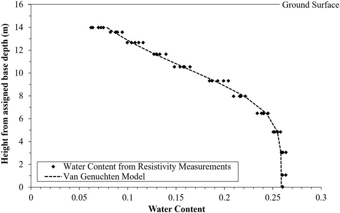
FIGURE 5. The normalized volumetric water content derived from vertical profiles of the ERI measurements. The dashed curve represents the fitted Van Genuchten (VG) model, which depicts the relationship between normalized water content and height from a presumed baseline.

We observed in Figure 5 that the vertical change in the water content shows a similar tendency to the Soil-Water Characteristic Curve (SWCC) obtained in lab tests, e.g., (Chin et al., 2010; Fredlund et al., 2011; Habasimbi and Nishimura, 2018; Azmi et al., 2019; Eyo et al., 2022). Hence, if we assume that the suction head is linearly proportional to the elevation of the groundwater level in the unconfined aquifer as discussed in Krahn and Fredlund (1972) and Stephens (2018), we then can estimate the groundwater level quantitatively and the relative hydraulic parameters in the vadose zone with the SWCC model. We applied the Van Genuchten (VG) model (Genuchten, 1980) that describes the physical relationship between the water contents and suction in the vadose zone through the following equation:

$\mathit{\theta }\left(\mathit{h}\right)={\mathit{\theta }}_{\mathit{r}}+\frac{\left({\mathit{\theta }}_{\mathit{s}}-{\mathit{\theta }}_{\mathit{r}}\right)}{{\left[\mathbf{1}+{\left(\mathit{\alpha }\mathit{h}\right)}^{\mathit{n}}\right]}^{\mathit{m}}};\mathit{w}\mathit{h}\mathit{e}\mathit{r}\mathit{e};\mathit{m}=\mathbf{1}-\mathbf{1}/\mathit{n}(6)$

Eq. 6 has four independent parameters, such as ${\theta }_s$, ${\theta }_r$, $\alpha$, and $n$ that need to be estimated from observed SWCC. Where ${\theta }_s$ is the saturated water content (L³/L³); ${\theta }_r$ is the residual water content (L³/L³); $\alpha$ is a parameter related to the air entry pressure (L⁻¹), and $n$ is a dimensionless parameter related to the pore-size distribution of soil and $h$ is the suction head (L). Furthermore, with the VG model of SWCC, we were able to estimate the air entry suction head relative to the same base (h_a), if we designate a saturated base with a depth of (H_s) and assume that the section head is proportional to the height of the presumed saturated base. Thus, it is possible to calculate the depth of the groundwater table (D):

$\mathit{D}={\mathit{H}}_{\mathit{s}}-{\mathit{h}}_{\mathit{a}}(7)$

We could invert the VG parameters and the air entry suction or heights from the base depth by minimizing the root mean square differences between the estimated and measured water content. To optimize the minimum object equation in the inversion, we utilized the Generalized Reduced Gradient (GRG) nonlinear program. Once we determined the groundwater depth, we advanced to estimate the groundwater level (GWL) by subtracting D from the ground level (G_L), expressed as:

$\mathit{G}\mathit{W}\mathit{L}={\mathit{G}}_{\mathit{l}}-\mathit{D}(8)$

In addition, we can obtain the theoretical specific yield, S_y (Eq. 9) by subtracting the residual water content from the saturated water content and the specific yield capacity, S_c (Eq. 10) with the VG model in Eq. 6, as:

${\mathit{S}}_{\mathit{y}}={\mathit{\theta }}_{\mathit{s}}-{\mathit{\theta }}_{\mathit{r}}(9)$

${\mathit{S}}_{\mathit{c}}=\frac{\mathbf{1}}{\mathit{D}}{\int }_{\mathbf{0}}^{\mathit{D}}\left({\mathit{\theta }}_{\mathit{s}}-\mathit{\theta }\left(\mathit{h}\right)\right)\mathit{d}\mathit{D}\cong \frac{\mathbf{1}}{\mathit{D}}{\displaystyle \sum _{\mathbf{0}}^{\mathit{D}}}\left({\mathit{\theta }}_{\mathit{s}}-\mathit{\theta }\left(\mathit{h}\right)\right)∆\mathit{D}(10)$

where $\theta \left(h\right)$ is the volumetric water content at a different depth, h, and $∆D$ is the incremental depth (Chang et al., 2022). We will discuss the S_y and S_c later in the discussion.

2.4 Time series clustering analysis (TSC)

Time series clustering (TSC) is an unsupervised machine-learning technique for identifying and grouping similar objects or data points into structures that are easier to understand. This technique is useful and capable of enhancing the interpretation and provides an intuitive explanation of relevant aspects of given time series datasets. Accordingly, it may lead us to discover interesting patterns that can be either frequent or rare patterns (Aghabozorgi et al., 2015; Rodriguez et al., 2019). A primary benefit associated with a TSC solution is its ability to automatically recover from failures, thereby eliminating the need for user intervention, compared to classification, the TSC not required prior information as label data. However, TSC entails certain drawbacks, namely, its inherent complexity and the inability to recover from database corruption. To address this limitation, the PCA (Principal Component Analysis) technique is utilized to reduce complexity, and preliminary data preparation steps are applied to prevent database corruption, such as removing blank data. The outcome of this method is the generation of a clustered resistivity value, which is determined based on its similarity to other values. This clustering allows for the identification and analysis of noteworthy patterns.

In this study, we attempted to use Hierarchical Agglomerative Clustering (HAC) by using the Orange data mining toolbox in python (Demsa et al., 2013). The toolbox effectively aids our aim to group synchronous and linearly correlated series or similarities in time. We were able to accomplish two tasks by utilizing such a technique: first, we managed to explain the trend of each site based on the VG model parameters over time in the area, and second, to describe the variation of groundwater level changes over time in the area. Nevertheless, TSC can be challenging due to the enormous complexity or dimensionality of the time series datasets. For instance, the second task dataset has a higher dimension (7200 × 4) compared to the first task dataset (50 × 3), therefore dimensionality reduction is necessary to conduct for the second task before applying the HAC, i.e., Principal Component Analysis (PCA).

2.4.1 Principal component analysis (PCA)

Principal Component Analysis (PCA) is a widely used algorithm prominently for dimensionality reduction. It useful to identify patterns in the dataset based on the correlation between its features. This projection-based method transforms the dataset (features) by projecting them onto a new subspace with equal or lower dimensions while keeping the essence of the original data. This step has several advantages, including reduced memory consumption and speed-up the clustering, noise reduction, and the harmonization of unequal data length or resolution, and the disadvantages of this method is that data standardization is a prerequisite before implementing PCA. This requirement introduces an additional step in the process. Furthermore, in order to apply PCA, all categorical features need to be converted into numerical features through standardization (Delforge et al., 2021). To assign equal weights (contributes equally) to the original dataset throughout the analysis phase, data standardization is compulsory prior to PCA, i.e., Z-standardization. Mathematically, this can be done by subtracting the mean $\left(\mu \right)$ from the individual data $\left(X\right)$ and dividing by the standard deviation $\left(\sigma \right)$:

${\mathit{X}}_{\mathit{z}}=\frac{\mathit{X}-\mathit{\mu }}{\mathit{\sigma }}(11)$

The outcome of PCA is a smaller set of summary indices. We refer the readers to Salem and Hussein. (2019) for the comprehensive principles and procedures of the PCA.

2.4.2 Hierarchical agglomerative clustering (HAC)

HAC is a technique that uses bottom-up approaches which start with single data as a single cluster and merge them until one big cluster remains. The necessary procedure in order to accomplish the goal involves data preparation, similarity measures, and linkage criteria (Dumont et al., 2018; Delforge et al., 2021; Puntu et al., 2021). HAC exhibits several advantages over other algorithms. Firstly, its implementation is straightforward. Secondly, it can generate a meaningful ordering of objects, facilitating visual representation through dendrograms. Additionally, HAC provides comprehensive insights into the degree of similarity among individual observations. Furthermore, it eliminates the need for pre-specifying the number of clusters or relying on pre-labeled data. Nevertheless, the algorithms also possess certain disadvantages. For instance, once a certain step is executed, it cannot be reversed or undone. In the event of new data being introduced, the entire process must be initiated again from the beginning. Furthermore, as HAC is a component of TSC, it inherits inherent complexity and lacks the capability to recover from database corruption. Certainly, in this study, we have taken into consideration all these limitations by thoroughly preparing the data and employing a dimensionality reduction technique like PCA.

The dataset is prepared in a way where the rows represent the observations and the columns represent the features or variables. For the first task (VG model), there are three features that act as data inputs: a, n, and S_c for all measurements. a and n are the fitting shape parameters related to the air entry pressure and the pore-size distribution, respectively. S_c (Specific Yield Capacity) was included in the algorithm to simplify the relationship between the residual and saturated water contents. For the second task (Groundwater Level Variation), the feature is the groundwater level difference against the measurement of the previous month, such as the GWL difference between May-February, July-May, September-July, and October-September (4 Features).

The Euclidean distance was chosen for the similarity measures to determine which clusters should be combined. It is the square root of the sum of the square differences:

${\mathit{d}}_{\left(\mathit{Q}\mathit{i},\mathit{Q}\mathit{j}\right)}=\sqrt{{\left({\mathit{Q}\mathbf{1}}_{\mathit{x}}-{\mathit{Q}\mathbf{2}}_{\mathit{x}}\right)}^{\mathbf{2}}+{\left({\mathit{Q}\mathbf{1}}_{\mathit{y}}-{\mathit{Q}\mathbf{2}}_{\mathit{y}}\right)}^{\mathbf{2}}}(12)$

where d is the Euclidean distance, x and y are the row index, and Q is the point data. Note that the distance between two objects is 0 when they are perfectly correlated.

Furthermore, the linkage criteria determined the distance between sets of observations as a function of the pairwise distances between them. This study focuses on the ward linkage method (Ward, 1963) that minimizes the total within-cluster variance, express as:

${\mathit{d}}_{\left(\mathit{u},\mathit{v}\right)}={\mathit{\delta }}^{\mathbf{2}}\left(\mathit{u},\mathit{v}\right)=\frac{\left|\mathit{u}\right|\left|\mathit{v}\right|}{\left|\mathit{u}\right|+\left|\mathit{v}\right|}{‖\mathit{u}-\mathit{v}‖}^{\mathbf{2}}(13)$

where u and v are the cluster data. HAC provides a nested structure of the clustering where all the sequences of merges are recorded into a tree-like diagram called a dendrogram. The results of HAC yield clustered data, organized according to their similarity, with the aim of identifying patterns and characteristics exhibited by each data group.

2.4.3 Time series clustering evaluation

Since the clustering method is an unsupervised method where the ground-truth labels are usually unavailable, an essential question that one should consider is how many clusters are suitable to describe the dataset. To evaluate the optimal number of clusters (k), we performed the Silhouette Index (SI), a method that measures how similar the data is to other data in the same cluster (cohesion and compactness) in comparison with the data of other clusters (separability) (Dudek, 2020; Delforge et al., 2021; Puntu et al., 2021). Mathematically, we write it down as:

$\mathit{S}\mathit{I}=\frac{\mathbf{1}}{\mathit{n}}{\displaystyle \sum _{\mathit{i}=\mathbf{1}}^{\mathit{n}}}\frac{\mathit{b}\left(\mathit{i}\right)-\mathit{a}\left(\mathit{i}\right)}{\mathit{max}\left\{\mathit{a}\left(\mathit{i}\right);\mathit{b}\left(\mathit{i}\right)\right\}},\mathit{S}\mathit{I}\in \left[-\mathbf{1},\mathbf{1}\right](14)$

$a\left(i\right)$ stands for the average distance from data i to other data belongings to its own cluster $\left(P_r\right)$; (data i belongs to cluster $P_r$), and $b\left(i\right)$ stands for the average distance from data i to other data belongings to neighborhood cluster $\left(P_s\right)$; (data i does not belong to cluster $P_s$), expressed as:

$\mathit{a}\left(\mathit{i}\right)={\sum }_{\mathit{k}\in \left\{{\mathit{P}}_{\mathit{r}}\backslash \mathit{i}\right\}}{\mathit{d}}_{\mathit{i}\mathit{k}}/\left({\mathit{n}}_{\mathit{r}}-\mathbf{1}\right)(15)$

$\mathit{b}\left(\mathit{i}\right)=\underset{\mathit{s}\ne \mathit{r}}{\mathit{min}}\left\{{\mathit{d}}_{\mathit{i}{\mathit{P}}_{\mathit{s}}}\right\},{\mathit{d}}_{\mathit{i}{\mathit{P}}_{\mathit{s}}}={\sum }_{\mathit{k}\in {\mathit{P}}_{\mathit{s}}}{\mathit{d}}_{\mathit{i}\mathit{k}}/{\mathit{n}}_{\mathit{s}}(16)$

where $d_{ik}$ and $d_{i{P}_s}$ are distance matrix, $n_r$ and $n_s$ are the number of data in cluster $P_r$ and $P_s$, respectively.

3 Results

3.1 The time-lapse ERI surveys

Five period of ERI surveys were carried out at ten sites in the Taichung-Nantou Basin along the Wu River in 2018. Figure 6 shows the inverted resistivity images for the ten sites, and Figure 7 shows the time-lapse resistivity images collected at the WS05 site.

FIGURE 6

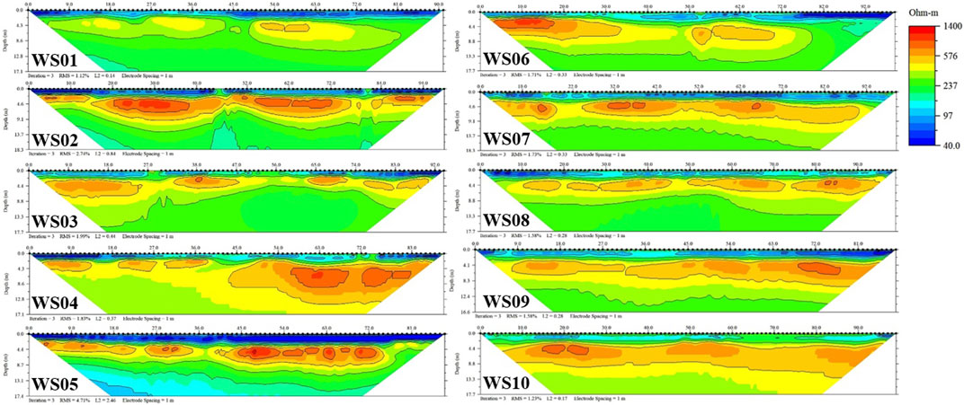
FIGURE 6. The inverted resistivity images of the survey lines in the Taichung-Nantou Basin along the Wu River during 2018.

FIGURE 7

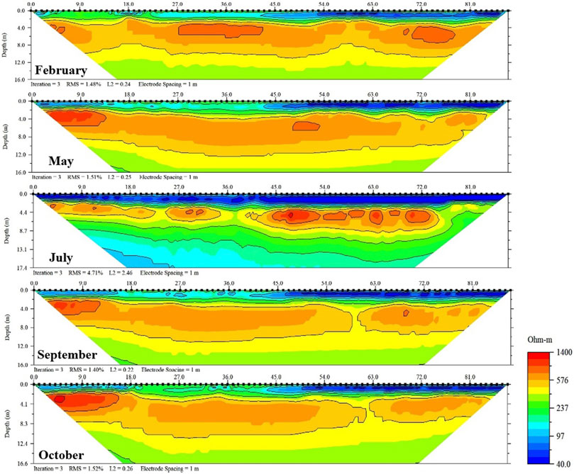
FIGURE 7. The time-lapse resistivity images collected at site WS05.

WS01 to WS04 sites are located on the northern part of the Wu River, while WS05 to WS10 sites are located on the southern part of the Wu River and the northern part of the Maoluo River, as shown in Figure 3. In general, the resistivity values vary in the range of 40 to 1,400 Ωm. The topmost 2 m layer with low resistivity anomaly from 40 to 100 Ωm (bluish color) represents the soil layer of the paddy field. Thus, we excluded this layer in order to estimate the normalized water content (see Section 2.3). Below this layer, the resistivity increases to over 400 Ωm until a certain depth (yellowish to reddish colors) that mostly lies around 8 m depth. At some point, the resistivity decreases from the peak of over 1,000 Ωm to a level between 200 and 300 Ωm. Such trend may reflect the effect of the increasing water content from the lower vadose zone to the saturation zone (transition zone). This resistivity trend is detected in every survey line. This implies that the study area lies on the same lithological formation, i.e., Sand, Clay and Gravel (see Section 2.1). Interestingly, the inverted resistivity images located nearby the confluence of two rivers (WS01 and WS05) are dominated by blue and green contour colors (low resistivity), while the WS04 and WS10 located on the upper course are dominated by yellow and red contour colors (high resistivity).

The inverted time-lapse resistivity images of WS05 collected in 2018 reveal a significant resistivity variation in the vadose zone between the dry and the wet seasons. The region with a high resistivity value (>500 Ωm) shrank from February to July indicating the water content in the vadose zone increased due to an increase in rainfall recharge. Meanwhile, the region with a low resistivity value (<150 Ωm) expanded from July to October owing to limited rainfall. The inverted resistivity image on July (wet season) shows the lowest resistivity distribution compared to others since the accumulated precipitation was the highest at about 334 m·mm/month (see Section 2.1). To observe the significant difference in the resistivity distribution, the resistivity values for each month were subtracted from the resistivity value of the dry season (February), and the results are shown in Figure 8. These results highlighted that the resistivity value plummeted from February to July (>50%) especially in the vadose zone owing to significant accumulated precipitation. On the other hand, May-February only shows slight resistivity changes up to 25% in the top-right corner of the section. The same trend is also observed in September-February and October-February with resistivity change of up to 30% and 15%, respectively. The resistivity variations in the dry and wet seasons can be linked to changes of the water content in the vadose zone, as was what stated in Archie’s law in Eq. 1. Thus, we were able to estimate further the variation of water contents and the groundwater table with the inverted resistivity images collected in different seasons.

FIGURE 8

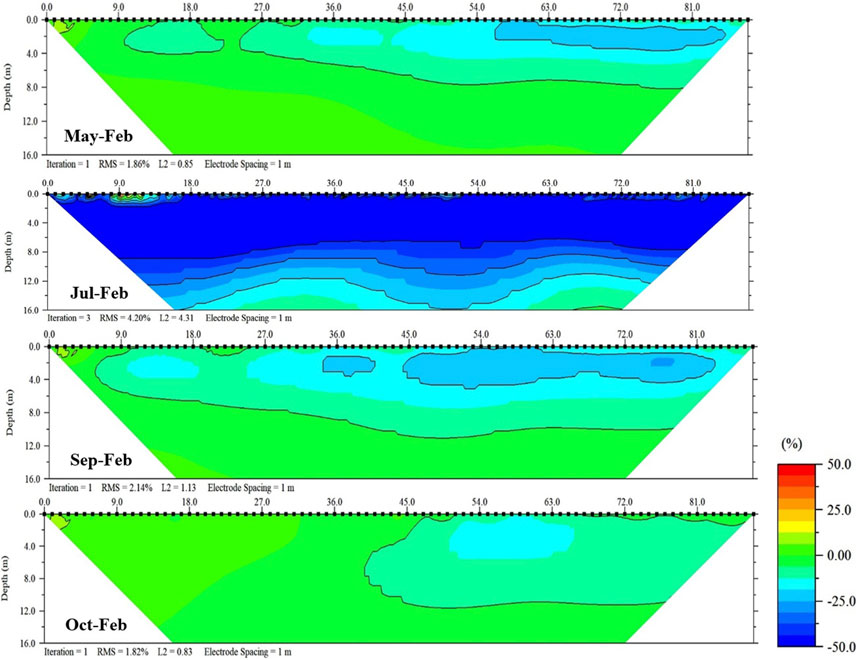
FIGURE 8. The resistivity differences distribution from each month against the dry season (February).

3.2 The inverted Van Genuchten model

Figure 9 presents the fitted VG model for different months at the survey sites in the study area. Generally, the fitted curves during the wet season (blue, green and purple dashed curves) have higher air entry heights than those in the dry season (red and orange curves). Table 1 presents an example of the fitted parameters of the VG curve at the WS05. a varies from 7.33 to 10.46 m, n varies in the range of 1.52–3.12, and ${\theta }_r$ is about 0.05–0.1. In addition, we assumed that the saturated water content would be equal to the average porosity, 0.26, for each measurement.

FIGURE 9

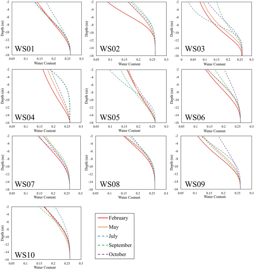
FIGURE 9. The fitted VG model for different months along the survey sites in the Taichung-Nantou Basin. The dashed curves indicate the models for the months in the wet season, and the solid curves are the fitted models for the months in the dry season.

TABLE 1

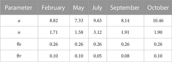
TABLE 1. The estimated parameters of the VG model from the time-lapse resistivity surveys at site WS05.

3.3 The estimation of groundwater levels

Table 2 lists the estimated groundwater levels (GWL) measured at different survey sites during the observation period in 2018. WS01-WS10 are the resistivity survey lines, while 98GH-06, 98GH-09, and 98GH-11 are the available observation wells around the survey area. The GWL covers a depth range of 22.9–51.4 m. The majority of the GWL are gradually increasing both in the observation wells and resistivity measurements from February to July due to an increase in recharge from the rainfall, in contrast to the GWL from July to October, which decreased owing to a decrease in recharge from the rainfall. To observe the spatial distribution trend of the GWL, the GWL were plotted onto the map. Figures 10A–E shows the spatial distribution of GWL for February, May, July, September, and October, respectively. The blue contour color stands for the high GWL, while the red contour color represents the low GWL.

TABLE 2

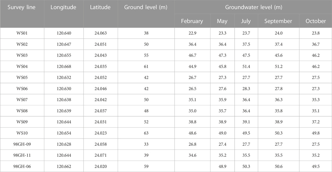
TABLE 2. The estimated groundwater levels were collected at survey sites and observation wells in 2018.

FIGURE 10

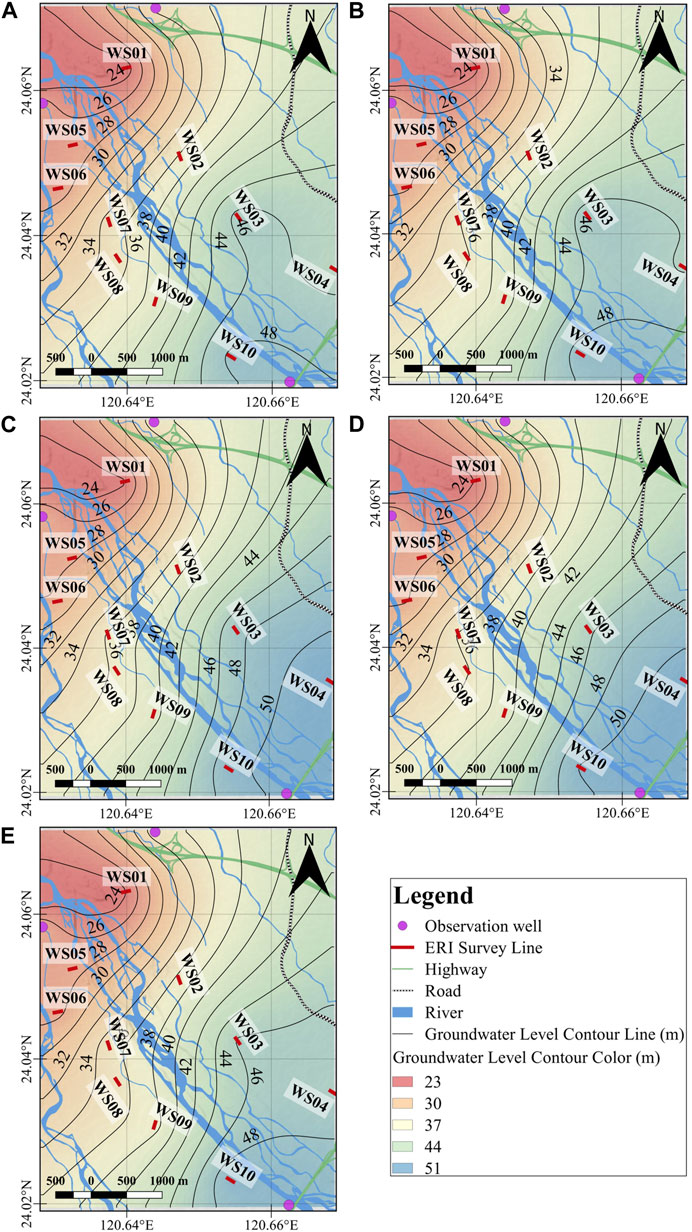
FIGURE 10. The spatial distributions of the groundwater levels in (A) February (the dry season), (B) May (the transition of dry-wet seasons), (C) July (the wet season), (D) September (the wet season), (E) October (the transition of wet-dry seasons) in 2018.

3.4 The estimation of specific yield

Aside from seasonal variations in groundwater levels, it is also vital to understand the water storage capacity of the region for potential groundwater reservoirs. Using Eqs 9, 10, we were able to estimate the theoretical specific yield, S_y, and the specific yield capacity, S_c. The results are listed in Table 3. In this case, the maximum and average for each estimation from all measurements time were calculated. The maximum and average of the theoretical specific yield as well as those of the specific yield capacity are in the range of 0.16–0.25, 0.14–0.24, 0.06–0.24, and 0.04–0.17, respectively. Figure 11 shows the spatial distribution of these estimations.

TABLE 3

TABLE 3. The estimated theoretical specific yields and specific yield capacities collected at ERI survey sites in 2018.

FIGURE 11

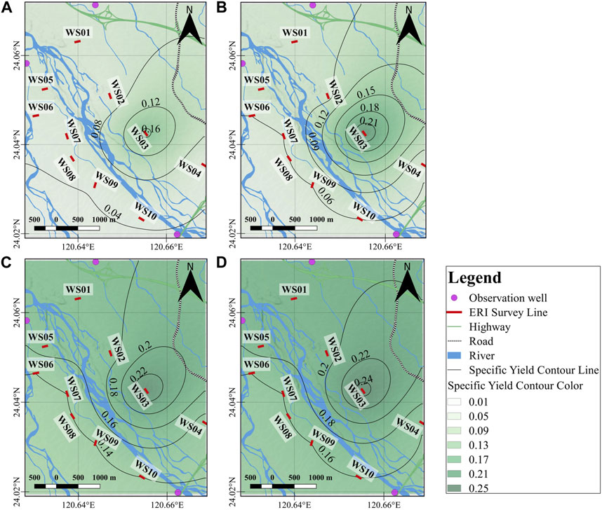
FIGURE 11. The distribution of (A) the average specific yield capacity, (B) maximum specific yield capacity, (C) average theoretical specific yield, (D) maximum theoretical specific yield during the study period.

3.5 The time series clustering results

3.5.1 The VG model parameters

In order to present the spatial distribution of TSC with the VG model parameters, we plotted the result onto the map as shown in Figure 12. The red dot, the green triangle, and the yellow diamond symbolize the cluster 1, cluster 2 and cluster 3, respectively. Table 4 lists the value of each cluster. The evaluation of this result with SI method is shown in Figure 13, in which the orange curve represents the average silhouette index (ASI) of the time series clustering for the VG model. In accordance to this curve, the optimal number of clusters (k) is 3, as it has the highest ASI value.

FIGURE 12

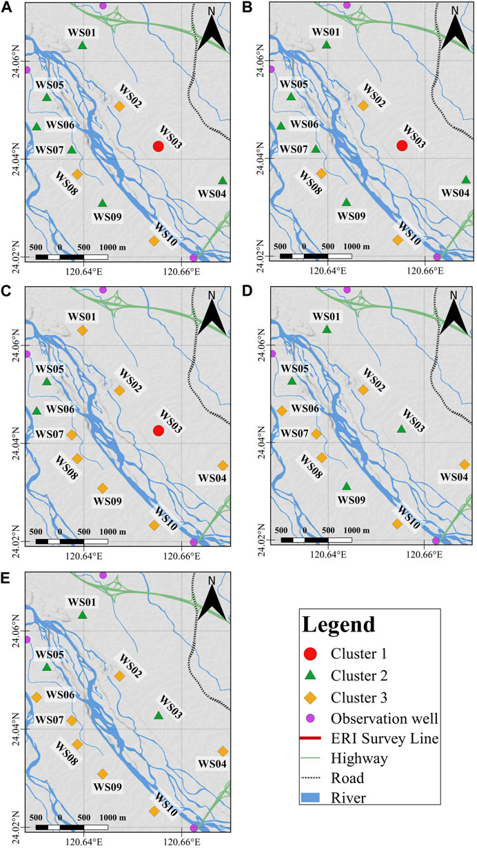
FIGURE 12. The distribution of the TSC result in (A) February (the dry season), (B) May (the transition of dry-wet seasons), (C) July (the wet season), (D) September (the wet season), (E) October (the transition of wet-dry seasons) in 2018.

TABLE 4

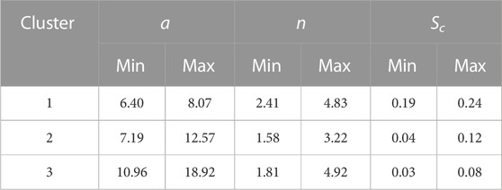
TABLE 4. The range of the a, n, and, S_c of each cluster for the Van Genuchten model.

FIGURE 13

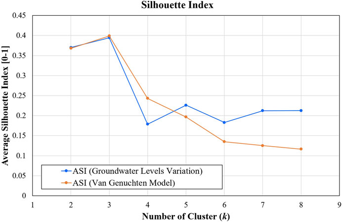
FIGURE 13. The Average Silhouette Index (ASI) of the TSC for groundwater levels variation (blue curve) and the Van Genuchten (VG) model (orange curve). Both curves show that the optimal number of clusters (k) for this data is 3.

3.5.2 The variation of groundwater level changes

PCA is applied prior to HAC for the dimensionality reduction of the datasets. To visualize the proportion of variance accounted for by each principal component (PC), the Scree plot is utilized (Ledesma et al., 2015). This is a graphical method that can be used to determine the number of Principal Components (PCs) to retain. Figure 14 shows the Scree plot, where the red line represents the component variance by each PC, and the blue line shows the cumulative variance. From this plot, we can read off the percentage of the variance in the data explained as we add PCs, the first PC explains roughly 55% of the variance of the data set, and the first two PCs explain about 80%, and so forth. Clearly, a bent point is observed at the first two PCs, which might indicate a good number of PCs to retain. Thus, the number of features is reduced from 4 to 2, while still retaining over 80% of the “information” contained within the original dataset. After PCA, the dataset is processed with HAC analysis. According to the highest ASI of the TSC result for the groundwater level variations (blue curve) in Figure 13, the optimal number of clusters (k) to describe the study data is three clusters (Table 5). Therefore, the spatial distribution of three clusters is plotted on the map, as shown in Figure 15. The red, green and blue rectangles are the cluster 1, cluster 2, and cluster 3, respectively.

FIGURE 14

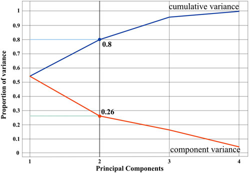
FIGURE 14. The Scree plot to visualize the proportion of the variance accounted for by each principal component (PC), the first two PCs explained about 80% of the original dataset.

TABLE 5

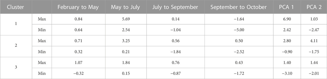
TABLE 5. The result from the HAC analysis for Groundwater Levels variations with three clusters.

FIGURE 15

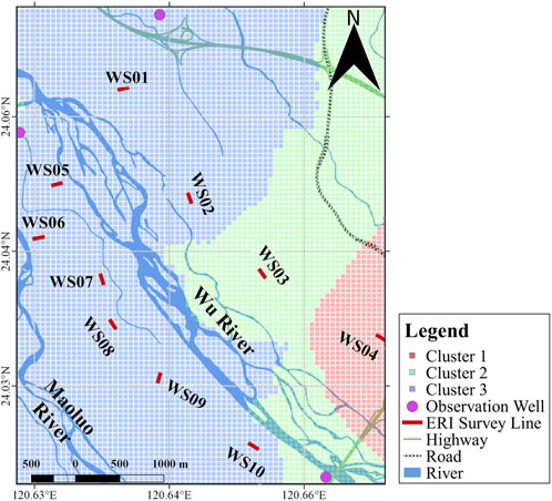
FIGURE 15. The spatial distribution of the three clusters obtained from the HAC analysis for the groundwater levels variation.

4 Discussion

We observed from Figure 10 that the GWL in the northwest of the study area is lower than in the southeast. This is reasonable since the ground level in the northwest is relatively lower than in the southeast. Correspondingly, the high GWL expanded from the southeast to the northwest during the period from February to July and reduced from July to October due to variations in recharge from rainfall events, which means the GWL will fluctuate mainly depending on the amount of rainfall. There is a good agreement between this trend and the inverted resistivity differences sections from each month against the dry season measurement (February) in Figure 8, where a significant decrease in resistivity is observed from the July-February period owing to the water content changes in the vadose zone, where GWL increased to higher levels.

To quantitatively establish areas of similar groundwater level changes during the study period, we applied multivariate analysis (HAC) to the groundwater level variation. Based on the SI method, the result suggests three clusters as the optimal number of groups. As shown in Figure 15, cluster 3 (blue rectangles) covers the majority of the study area, followed by cluster 2 (green rectangles), and cluster 1 (red rectangles). The variation of groundwater changes indicates that cluster 1 experienced a more significant change than its neighboring clusters. Table 5 demonstrates that the GWL of cluster 1 increased by about 5.69 m from the dry season to the wet season and dropped by about −5 m from the wet season to the dry season. The GWL of cluster 2 and 3 increased by about 3.25 and 1.84 m and dropped by about −2.52 and −1.72 m, respectively. In terms of spatial patterns, initially, we assumed that the area between the Wu River and the Maoluo River was divided in such a way that cluster 1 lies in the southeast, cluster 2 in the middle, and cluster 3 in the northwest, based on the GWL distribution that moved from the southeast to the northwest and vice versa each month (see Figure 10). However, further analysis of the GWL change with HAC revealed that cluster 1 covers this area, with only a few areas covered by cluster 2 in the southeast. Cluster 3 covers the rest of the area. This finding suggests a considerable change in GWL in the northern part of the Wu River channel compared to the southern area that parallels the Maoluo River.

Aside from monitoring the seasonal variations of GWL, we were also able to estimate the specific yield of the region, which is one of the essential hydrogeology parameters for qualitative and quantitative studies of groundwater resources, especially for locating potential groundwater reservoirs. Specific yield (S_y) denotes the maximum groundwater volume ratio that can be yielded or stored in an unconfined aquifer in a condition where it is completely dried. However, groundwater volume ratios that may be pumped from or stored in a sediment cannot exceed specific yield owing to capillary fringes in the vadose zone. Hence, in this study, we utilized Eq. 10 to calculate the specific yield capacity (S_c), which is a natural specific yield corresponding to the capillary fringes in the vadose zone. Figures 11A, B present the distribution of the average and maximum of S_c, whereas Figures 11C, D present the distribution of the average and maximum of S_y. Both S_c and S_y exhibit similar patterns where the maximum value is located in WS03, and the minimum value is located in WS04, and WS06-WS10. Nevertheless, the estimated value of S_c is lower for both average and maximum compared to S_y. These results are in line with Chang et al. (2022), who noted that the majority of the estimated specific yield capacity (S_c) value agreed with the value estimated from the in-situ pumping test, which is only three-quarters to two-thirds of the estimated theoretical specific yield (S_y). Furthermore, the estimated S_c range correlates favorably with previous studies by Huang et al. (2014) and Liu et al. (2018), in which the estimated specific yield in this area ranges from 0.01 to 0.1.

We applied the HAC algorithm to the VG model parameters as well, and the result can be seen in Figure 12. Since the S_c was one of the features of this algorithm, there was a positive correlation with the S_c distribution maps in Figure 11. The transition from the dry season to the wet season (Figures 12A–C) shows the aforementioned WS03 site with the highest S_c included in cluster 1 (a: 6.40–8.07, n: 2.41–4.83, and S_c: 0.19–0.24), and is included in cluster 2 (a: 7.19–12.57, n: 1.58–3.22, and S_c: 0.04–0.12) from the wet season to the dry season (Figures 12C–E). In contrast with the sites with low S_c (the WS04, WS06, WS07, WS08, WS09, and WS10 sites), the majority of them are included in cluster 2 and cluster 3 (a: 10.96–18.92, n: 1.81–4.92, and S_c: 0.03–0.08), where the WS08 and WS10 sites are constantly in cluster 3 during the study period. Interestingly, the WS05 site that is located closest to the confluence of the branches between the Wu and Maoluo Rivers is constantly in cluster 1 during the study period. In summary, the implementation of the HAC to the groundwater change variation and the VG model parameters suggests that the WS03 site is a promising area for further groundwater investigation since it has the highest S_c value with a slight change in groundwater levels during the study period under different seasonal conditions.

The Time-lapse ERI measurements provide reliable results for spatial groundwater monitoring in the survey region. These findings are confirmed by comparing the estimated GWL obtained from the ERI survey with the observed GWL from the nearest available observation wells along the river channel (Figure 16). There are three accessible observation wells in the study area, namely, 98GH-09, 98GH-06, and 98GH-11 (see Figure 3). The 98GH-09 well is in the northwest, the 98GH-06 well is in the southeast, and the 98GH-11 well is farther away from the river channel. Thus, the 98GH-09 and 98GH-06 wells were selected for comparison and validation.

FIGURE 16

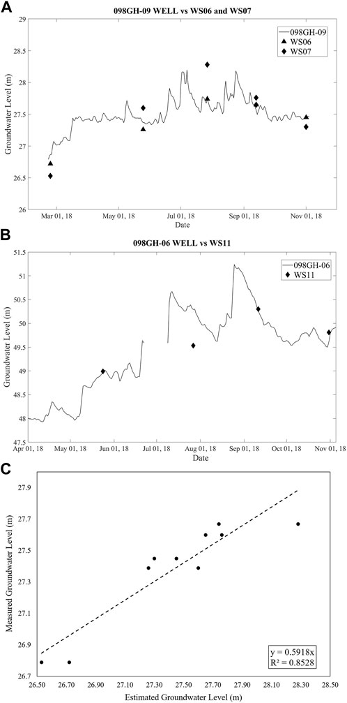
FIGURE 16. A comparison of the estimated and observed GWL at site WS05 and WS06 with observation well 098GH-09 (A), and site WS10 with observation well 098GH-06 (B). The correlation between the estimated and observed GWL with R2 of about 0.85 (C).

Figure 16A compares the 098GH-09 and the ERI WS05 and WS06 sites, whereas Figure 16B compares the 098GH-06 wells and the ERI WS10 site. Interestingly, on closer inspection of Figure 16A, the values of the observed GWL from WS05 (triangles) are more akin to the estimated GWL from the 098GH-09 well compared to the observed GWL from WS06 (diamonds). This difference is understandable since site WS05 location is only about 0.7 km away from observation well 098GH-09, while site WS06 is over 1 km away. Apart from this slight discordance, the result shows that the values do not highly diverge since the location of these sites is still in the same formation deposits, which are the alluvial deposits. Both figures also show that the estimated GWL is consistent with the measured GWL, where GWL increases from February to early September (the dry season to the wet season) and decreases afterward (the wet season to the dry season). On the other hand, Figure 16C demonstrates the correlation between estimated and observed GWL in WS05, WS06, and WS10 sites, where the coefficient of determination R² is about 0.85. This result shows good agreement between the estimated and observed GWL. Taken together, these results have further strengthened our confidence in using the ERI measurement as an alternative and effective method for monitoring seasonal groundwater level changes when observation wells are scarce or unavailable in the target area. Although the present study has yielded insights into applying the ERI method for groundwater monitoring, it is crucial to acknowledge certain limitations that can be addressed in future research. For instance, the technique employed in this study relies on surface electrodes, which may pose challenges in densely vegetated or urban areas, thereby limiting accessibility to specific regions. Consequently, conducting an initial survey of suitable locations becomes necessary. Additionally, the method is sensitive to near-surface conditions, such as vegetation, building foundations, or pathways through rice fields, which can introduce noise and artifacts into the data and affect the interpretation of subsurface groundwater properties. To cope with this issue, it is recommended to avoid such areas whenever possible. In cases where avoidance is not feasible, conducting pre-analysis with obtained raw data prior to the inversion process is suggested. Despite these limitations, our recent findings demonstrate the potential of the proposed method in monitoring groundwater conditions and estimating groundwater parameters under varying seasonal conditions.

5 Conclusion

We have applied Time-lapse Electrical Resistivity Imaging (TL-ERI) and Hierarchical Agglomerative Clustering (HAC) in machine learning for monitoring groundwater levels (GWL) and estimating specific yields in the Taichung-Nantou Basin along the Wu River, Central Taiwan. The findings of our study reveal that the GWL ranged from 22.9 to 51.4 m. During the dry-wet seasons (February to July), the GWL expanded from southeast to northwest and contracted from July to October (wet-dry seasons), primarily influenced by variations in recharge from rainfall events. Notably, the WS03 site exhibited the highest estimated specific yield capacity (S_c), with maximum and average values of approximately 0.24 and 0.17, respectively. Other sites had maximum and average values ranging from 0.06 to 0.09 and 0.04 to 0.07, respectively. Furthermore, the results from HAC indicate that the study area can be divided into three clusters. In cluster 1, the GWL increased by around 5.69 m from the dry season to the wet season and decreased by approximately −5 m from the wet season to the dry season. Clusters 2 and 3 experienced GWL increases of about 3.25 and 1.84 m, respectively, and GWL decreases of approximately −2.52 and −1.72 m, respectively. Additionally, a similar clustering algorithm was applied to the VG model parameters (a, n, and S_c) during the study period, revealing that the measurement sites can be grouped into three clusters. Cluster 1 exhibited parameter ranges of a: 6.40–8.07, n: 2.41–4.83, and S_c: 0.19–0.24. Cluster 2 had parameter ranges of a: 7.19–12.57, n: 1.58–3.22, and S_c: 0.04–0.12. Cluster 3 showed parameter ranges of a: 10.96–18.92, n: 1.81–4.92, and S_c: 0.03–0.08. Notably, WS03, the site with the highest S_c value, was the only site included in cluster 1. Overall, these findings suggest that WS03 is a promising area for further investigation of groundwater reservoirs, as it exhibits the highest S_c value with minimal fluctuations in groundwater levels during the dry and wet seasons. In summary, the TL-ERI method combined with time series clustering in machine learning offers a viable and efficient approach to monitor groundwater levels and estimate specific yields, particularly in situations where limited or no observation wells are available for specific or regional areas under varying seasonal conditions.

Data availability statement

The original contributions presented in the study are included in the article/Supplementary Material, further inquiries can be directed to the corresponding author.

Author contributions

JP: Conceptualization, writing-original draft, writing—review and editing, data curation, investigation, methodology, formal analysis, visualization. P-YC: Conceptualization, writing—review and editing, methodology, supervision. HA: Writing—review and editing, visualization, resources. D-JL: Investigation and resources. C-YS: Resources and data curation. MS: Investigation and visualization. L-CC: Funding acquisition and resources. YD: Resources. All authors contributed to the article and approved the submitted version.

Funding

This research was funded by the Central Geological Survey in the Ministry of Economic Affairs, R.O.C., under project number 107-5226904000-01-02-1.

Acknowledgments

The authors wish to express their sincere gratitude to the Near Surface Geophysics Research Group at National Central University, Taiwan for their valuable assistance rendered during this study, especially to Mr. Yu-Chang Wu. Furthermore, the authors extend their gratitude to the reviewers for their insightful feedback and suggestions that greatly contributed to the refinement of this work.

Conflict of interest

The authors declare that the research was conducted in the absence of any commercial or financial relationships that could be construed as a potential conflict of interest.

Publisher’s note

All claims expressed in this article are solely those of the authors and do not necessarily represent those of their affiliated organizations, or those of the publisher, the editors and the reviewers. Any product that may be evaluated in this article, or claim that may be made by its manufacturer, is not guaranteed or endorsed by the publisher.

Supplementary material

The Supplementary Material for this article can be found online at: https://www.frontiersin.org/articles/10.3389/fenvs.2023.1197888/full#supplementary-material

References

Aduojo, A. A., Ayolabi, E. A., and Adewale, A. (2018). Time dependent electrical resistivity tomography and seasonal variation assessment of groundwater around the Olushosun dumpsite Lagos, South-west, Nigeria. J. Afr. Earth Sci. 147, 243–253. doi:10.1016/j.jafrearsci.2018.06.024

CrossRef Full Text | Google Scholar

Advanced Geosciences (2006). Instruction manual for EarthImager 2D. Austin, TX, USA: Advanced Geosciences Inc.

Google Scholar

Aghabozorgi, S., Seyed Shirkhorshidi, A., and Ying Wah, T. (2015). Time-series clustering – a decade review. Inf. Syst. 53, 16–38. doi:10.1016/j.is.2015.04.007

CrossRef Full Text | Google Scholar

Akhter, G., Ge, Y., Hasan, M., and Shang, Y. (2022). Estimation of hydrogeological parameters by using pumping, laboratory data, surface resistivity and thiessen technique in lower bari doab (indus basin), Pakistan. Appl. Sci. 12 (6), 3055. doi:10.3390/app12063055

CrossRef Full Text | Google Scholar

Archie, G. E. (1942). The electrical resistivity log as an aid in determining some reservoir characteristics. Trans. AIME 146 (01), 54–62. doi:10.2118/942054-G

CrossRef Full Text | Google Scholar

Azmi, M., Ramli, M. H., Hezmi, M. A., Mohd Yusoff, S., and Alel, M. N. A. (2019). Estimation of Soil Water Characteristic Curves (SWCC) of mining sand using soil suction modelling. IOP Conf. Ser. Mater. Sci. Eng. 527, 012016. doi:10.1088/1757-899X/527/1/012016

CrossRef Full Text | Google Scholar

Bai, L., Huo, Z., Zeng, Z., Liu, H., Tan, J., and Wang, T. (2021). Groundwater flow monitoring using time-lapse electrical resistivity and Self Potential data. J. Appl. Geophys. 193, 104411. doi:10.1016/j.jappgeo.2021.104411

CrossRef Full Text | Google Scholar

Bai, T., Tsai, W. P., Chiang, Y. M., Chang, F. J., Chang, W. Y., Chang, L. C., et al. (2019). Modeling and investigating the mechanisms of groundwater level variation in the jhuoshui river basin of central taiwan. Water 11 (8), 1554. doi:10.3390/w11081554

CrossRef Full Text | Google Scholar

Chang, P. Y., Chang, L. C., Hsu, S. Y., Tsai, J. P., and Chen, W. F. (2017). Estimating the hydrogeological parameters of an unconfined aquifer with the time-lapse resistivity-imaging method during pumping tests: Case studies at the Pengtsuo and Dajou sites, Taiwan. J. Appl. Geophys. 144, 134–143. doi:10.1016/j.jappgeo.2017.06.014

CrossRef Full Text | Google Scholar

Chang, P. Y., Hsu, S. Y., Chang, L. C., Chen, W. F., Chen, Y. W., and Lu, H. Y. (2016). Using the resistivity imaging method to monitor the dynamic effects on the vadose zone during pumping tests at the pengtsuo site in pingtung, taiwan. Terr. Atmos. Ocean. Sci. 27 (1), 059. doi:10.3319/tao.2015.08.20.01(t

CrossRef Full Text | Google Scholar

Chang, P. Y., Puntu, J. M., Lin, D. J., Yao, H. J., Chang, L. C., Chen, K. H., et al. (2022). Using time-lapse resistivity imaging methods to quantitatively evaluate the potential of groundwater reservoirs. Water 14 (3), 420. doi:10.3390/w14030420

CrossRef Full Text | Google Scholar

Chen, H. S., Chen, K. S., Chen, C. Y., Hung, C. C., Meng, P. J., and Chen, M. H. (2021). Spatiotemporal distribution of shrimp assemblages in the Western coastal waters off taiwan at the tropic of cancer, western pacific ocean. Coast. Shelf Sci. 255, 107356. doi:10.1016/j.ecss.2021.107356

CrossRef Full Text | Google Scholar

Chen, T. T., Hsu, W. L., and Chen, W. K. (2020). An assessment of water resources in the taiwan strait island using the water poverty index. Sustainability 12 (6), 2351. doi:10.3390/su12062351

CrossRef Full Text | Google Scholar

Chin, K. B., Leong, E. C., and Rahardjo, H. (2010). A simplified method to estimate the soil-water characteristic curve. Can. Geotechnical J. 47 (12), 1382–1400. doi:10.1139/t10-033

CrossRef Full Text | Google Scholar

Dahlin, T., and Zhou, B. (2004). A numerical comparison of 2D resistivity imaging with 10 electrode arrays. Geophys. Prospect. 52 (5), 379–398. doi:10.1111/j.1365-2478.2004.00423.x

CrossRef Full Text | Google Scholar

Delforge, D., Watlet, A., Kaufmann, O., Van Camp, M., and Vanclooster, M. (2021). Time-series clustering approaches for subsurface zonation and hydrofacies detection using a real time-lapse electrical resistivity dataset. J. Appl. Geophys. 184, 104203. doi:10.1016/j.jappgeo.2020.104203

CrossRef Full Text | Google Scholar

Demsa, J., Meng, P. J., and Chen, M. H. (2013). Orange: Data mining toolbox in Python. J. Mach. Learn. Res. 14, 2349–2353. doi:10.5555/2567709.2567736

CrossRef Full Text | Google Scholar

Dibaj, M., Javadi, A. A., Akrami, M., Ke, K. Y., Farmani, R., Tan, Y. C., et al. (2020). Modelling seawater intrusion in the Pingtung coastal aquifer in Taiwan, under the influence of sea-level rise and changing abstraction regime. Hydrogeology J. 28 (6), 2085–2103. doi:10.1007/s10040-020-02172-4

CrossRef Full Text | Google Scholar

Dietrich, S., Carrera, J., Weinzettel, P., and Sierra, L. (2018). Estimation of specific yield and its variability by electrical resistivity tomography. Water Resour. Res. 54 (11), 8653–8673. doi:10.1029/2018wr022938

CrossRef Full Text | Google Scholar

Dudek, A. (2020). “Silhouette index as clustering evaluation tool,” in Classification and data analysis (Midtown Manhattan, New York City: Springer, Cham), 19–33.

CrossRef Full Text | Google Scholar

Dumont, M., Reninger, P., Pryet, A., Martelet, G., Aunay, B., and Join, J. (2018). Agglomerative hierarchical clustering of airborne electromagnetic data for multi-scale geological studies. J. Appl. Geophys. 157, 1–9. doi:10.1016/j.jappgeo.2018.06.020

CrossRef Full Text | Google Scholar

Eyo, E. U., Ng'ambi, S., and Abbey, S. (2022). An overview of soil–water characteristic curves of stabilised soils and their influential factors. J. King Saud Univ. Eng. Sci. 34 (1), 31–45. doi:10.1016/j.jksues.2020.07.013

CrossRef Full Text | Google Scholar

Fredlund, D. G., Sheng, D., and Zhao, J. (2011). Estimation of soil suction from the soil-water characteristic curve. Can. Geotechnical J. 48 (2), 186–198. doi:10.1139/t10-060

CrossRef Full Text | Google Scholar

Genuchten, V. (1980). A closed-form equation for predicting the hydraulic conductivity of unsaturated soils. Soil Sci. Soc. Am. J. 44 (5), 892–898. doi:10.2136/sssaj1980.03615995004400050002x

CrossRef Full Text | Google Scholar

Glover, P. W. J. (2015). “Geophysical properties of the near surface earth: Electrical properties,” in Treatise on Geophysics (Amsterdam: Elsevier), 89–137.

CrossRef Full Text | Google Scholar

Gopinathan, P., Nandini, C., Parthiban, S., Sathish, S., Singh, A. K., and Singh, P. K. (2020). A geo-spatial approach to perceive the groundwater regime of hard rock terrain-a case study from Morappur area, Dharmapuri district, South India. Groundw. Sustain. Dev. 10, 100316. doi:10.1016/j.gsd.2019.100316

CrossRef Full Text | Google Scholar

Habasimbi, P., and Nishimura, T. (2018). Comparison of soil–water characteristic curves in one-dimensional and isotropic stress conditions. Soil Syst. 2 (3), 43. doi:10.3390/soilsystems2030043

CrossRef Full Text | Google Scholar

Han, Z., Huang, S., Huang, Q., Leng, G., Wang, H., Bai, Q., et al. (2019). Propagation dynamics from meteorological to groundwater drought and their possible influence factors. J. Hydrology 578, 124102. doi:10.1016/j.jhydrol.2019.124102

CrossRef Full Text | Google Scholar

Hasan, M., Shang, Y., Jin, W., and Akhter, G. (2020). Estimation of hydraulic parameters in a hard rock aquifer using integrated surface geoelectrical method and pumping test data in southeast Guangdong, China. Geosciences J. 25 (2), 223–242. doi:10.1007/s12303-020-0018-7

CrossRef Full Text | Google Scholar

Ho, H. C., and Chen, M. M. (2000). Explanatory text of the geological map of taiwan scale 1:50.000 sheet 24. New Taipei City: Central Geological Survey of Taiwan.

Google Scholar

Hsu, Y. J., Fu, Y., Bürgmann, R., Hsu, S. Y., Lin, C. C., Tang, C. H., et al. (2020). Assessing seasonal and interannual water storage variations in Taiwan using geodetic and hydrological data. Earth Planet. Sci. Lett. 550, 116532. doi:10.1016/j.epsl.2020.116532

CrossRef Full Text | Google Scholar

Huang, C. C., Lin, C. C., and Tang, C. H. (2014). Analysis and Application of the Pumping test of the mountain area- A case Study in the middle Section of western taiwan. [山區岩層抽水試驗分析及應用-以台灣西部中段山區為例]. Sinotech Eng. 122, 45–52. doi:10.30154/SE

CrossRef Full Text | Google Scholar

Huang, W. C., Chiang, Y., Wu, R. Y., Lee, J. L., and Lin, S. H. (2012). The impact of climate change on rainfall frequency in taiwan. Terr. Atmos. Ocean. Sci. 23 (5), 553. doi:10.3319/tao.2012.05.03.04(WMH)

CrossRef Full Text | Google Scholar

Hung, C. W., and Shih, M. F. (2019). Analysis of severe droughts in taiwan and its related atmospheric and oceanic environments. Atmosphere 10 (3), 159. doi:10.3390/atmos10030159

CrossRef Full Text | Google Scholar

Hung, W. C., Hwang, C., Chen, Y. A., Zhang, L., Chen, K. H., Wei, S. H., et al. (2017). Land subsidence in chiayi, taiwan, from compaction well, leveling and ALOS/PALSAR: Aquaculture-induced relative sea level rise. Remote Sens. 10 (2), 40. doi:10.3390/rs10010040

CrossRef Full Text | Google Scholar

Hwang, J. S. (2003). The development and management policy of water resources in Taiwan. Paddy Water Environ. 1 (3), 115–120. doi:10.1007/s10333-003-0019-y

CrossRef Full Text | Google Scholar

Krahn, J., and Fredlund, D. G. (1972). On total, matric and osmotic suction. Soil Sci. 114 (5), 339–348. doi:10.1097/00010694-197211000-00003

CrossRef Full Text | Google Scholar

Lech, M., Skutnik, Z., Bajda, M., and Markowska-Lech, K. (2020). Applications of electrical resistivity surveys in solving selected geotechnical and environmental problems. Appl. Sci. 10 (7), 2263. doi:10.3390/app10072263

CrossRef Full Text | Google Scholar

Ledesma, R. D., Valero-Mora, P., and Macbeth, G. (2015). The scree test and the number of factors: A dynamic graphics approach. Span. J. Psychol. 18, E11. doi:10.1017/sjp.2015.13

PubMed Abstract | CrossRef Full Text | Google Scholar

Lee, C. H., Chen, W. P., and Lee, R. H. (2006). Estimation of groundwater recharge using water balance coupled with base-flow-record estimation and stable-base-flow analysis. Environ. Geol. 51 (1), 73–82. doi:10.1007/s00254-006-0305-2

CrossRef Full Text | Google Scholar

Lippman, E. (2014). Four-point Ligh10W earth resistivity meter ver. 4.58. Schaufling, Germany: Lipmann Geophysikalische Messgeräte.

Google Scholar

Liu, H. J., Xiao, T., Yang, J. H., Qin, Y., and Gao, J. J. (2018). Parthenolide attenuated bleomycin-induced pulmonary fibrosis via the NF-κB/Snail signaling pathway. Taiwan Assoc. Hydraulic Eng. 6, 111–127. doi:10.1186/s12931-018-0806-z

CrossRef Full Text | Google Scholar

Perdomo, S., Kruse, E. E., and Ainchil, J. E. (2018). Estimation of hydraulic parameters using electrical resistivity tomography (ERT) and empirical laws in a semi-confined aquifer. Near Surf. Geophys. 16 (6), 627–641. doi:10.1002/nsg.12020

CrossRef Full Text | Google Scholar

Puntu, J. M., Chang, P. Y., Lin, D. J., Amania, H. H., and Doyoro, Y. G. (2021). A comprehensive evaluation for the tunnel conditions with ground penetrating radar measurements. Remote Sens. 13 (21), 4250. doi:10.3390/rs13214250

CrossRef Full Text | Google Scholar

Ramsahoye, L., and Lang, S. M. (1961). A simple method for determining specific yield from pumping tests. USA: US Government Printing Office.

Google Scholar

Rodriguez, M. Z., Comin, C. H., Casanova, D., Bruno, O. M., Amancio, D. R., Costa, L. D. F., et al. (2019). Clustering algorithms: A comparative approach. PLoS One 14 (1), e0210236. doi:10.1371/journal.pone.0210236

PubMed Abstract | CrossRef Full Text | Google Scholar

Salem, N., and Hussein, S. (2019). Data dimensional reduction and principal components analysis. Procedia Comput. Sci. 163, 292–299. doi:10.1016/j.procs.2019.12.111

CrossRef Full Text | Google Scholar

Sharma, S., and Verma, G. K. (2015). Inversion of electrical resistivity data: A review. Int. J. Comput. Syst. Eng. 9 (4), 400–406. doi:10.5281/zenodo.1106169

CrossRef Full Text | Google Scholar

Stephens, D. B. (2018). Vadose zone hydrology. Boca Raton: CRC Press.

Google Scholar

Taylor, C. J., and Alley, W. M. (2001). Ground-water-level monitoring and the importance of long-term water-level data (Vol 1217). USA: US Geological Survey Denver, CO.

Google Scholar

Tesfaldet, Y. T., and Puttiwongrak, A. (2019). Seasonal groundwater recharge characterization using time-lapse electrical resistivity tomography in the thepkasattri watershed on phuket island, Thailand. Hydrology 6 (2), 36. doi:10.3390/hydrology6020036

CrossRef Full Text | Google Scholar

Wahab, S., Saibi, H., and Mizunaga, H. (2021). Groundwater aquifer detection using the electrical resistivity method at Ito Campus, Kyushu University (Fukuoka, Japan). Geosci. Lett. 8 (1), 15. doi:10.1186/s40562-021-00188-6

CrossRef Full Text | Google Scholar

Wang, S. J., Lee, C. H., Yeh, C. F., Choo, Y. F., and Tseng, H. W. (2021). Evaluation of climate change impact on groundwater recharge in groundwater regions in taiwan. Water 13 (9), 1153. doi:10.3390/w13091153

CrossRef Full Text | Google Scholar

Ward, J. H. (1963). Hierarchical grouping to optimize an objective function. J. Am. Stat. Assoc. 58 (301), 236–244. doi:10.1080/01621459.1963.10500845

CrossRef Full Text | Google Scholar

Yeh, H. F., and Hsu, H. L. (2019). Using the Markov chain to analyze precipitation and groundwater drought characteristics and linkage with atmospheric circulation. Sustainability 11 (6), 1817. doi:10.3390/su11061817

CrossRef Full Text | Google Scholar