Multiscale phenology of seasonally dry tropical forests in an aridity gradient

The leaf phenology of seasonally dry tropical forests (SDTFs) is highly seasonal, marked by synchronized flushing of new leaves triggered by the first rains of the wet season. Such phenological transitions may not be accurately detected by remote sensing vegetation indices and derived transition dates (TDs) due to the coarse spatial and temporal resolutions of satellite data. The aim of this study was to compared TDs from PhenoCams and satellite remote sensing (RS) and used the TDs calculated from PhenoCams to select the best thresholds for RS time series and calculate TDs. For this purpose, we assembled cameras in seven sites along an aridity gradient in the Brazilian Caatinga, a region dominated by SDTFs. The leafing patterns were registered during one to three growing seasons from 2017 to 2020. We drew a region of interest (ROI) in the images to calculate the normalized green chromatic coordinate index. We compared the camera data with the NDVI time series (2000–2019) derived from near-infrared (NIR) and red bands from MODIS product data. Using calibrated PhenoCam thresholds reduced the mean absolute error by 5 days for SOS and 34 days for EOS, compared to common thresholds in land surface phenology studies. On average, growing season length (LOS) did not differ significantly among vegetation types, but the driest sites showed the highest interannual variation. This pattern was applied to leaf flushing (SOS) and leaf fall (EOS) as well. We found a positive relationship between the accumulated precipitation and the LOS and between the accumulated precipitation and maximum and minimum temperatures and the vegetation productivity (peak and accumulated NDVI). Our results demonstrated that (A) the fine temporal resolution of phenocamera phenology time series improved the definitions of TDs and thresholds for RS landscape phenology; (b) long-term RS greening responded to the variability in rainfall, adjusting their timing of green-up and green-down, and (C) the amount of rainfall, although not determinant for the length of the growing season, is related to the estimates of vegetation productivity.

1 Introduction

Phenological data have been successfully used to understand ecological aspects from the individual level, as in plant–animal interactions (Morellato et al., 2016), to the ecosystem level, in terms of the role of vegetation dynamics in driving carbon and energy fluxes (Reich, 1995; Polgar and Primack, 2011; Richardson et al., 2013). The newly realized potential of phenology as a monitoring tool, in tandem with recent advances in technology, has enabled the use of automated phenological monitoring techniques at different levels of observation (Morellato et al., 2016; Alberton et al., 2017; Albernethy et al., 2018; Piao et al., 2019). New digital near-remote sensing sensors have proven to effectively monitor multiple sites (Richardson et al., 2018) while advancing in answering key ecological questions even for tropical regions (Alberton et al., 2014; Alberton et al., 2017; Alberton et al., 2019; Paloschi et al., 2020; Alberton et al., 2023; Medeiros et al., 2023; Wang et al., 2023).

Land surface phenology (LSP) works with satellite imagery collections from a wide variety of orbital sensors. Among the most commonly applied mechanisms to track long-term leafing trends are the MODIS products (Huete et al., 2002; Khare et al., 2022). The derived time series of vegetation indices (VIs), such as enhanced vegetation index (EVI) and normalized difference vegetation index (NDVI), is the base for calculations of the phenological metrics that define the growing seasons, such as the start of season (SOS), the peak of season (POS), and the end of season (EOS), that in general correspond to the green-up, maturity, and senescence stages of a target vegetation (Zhang et al., 2003; Tuanmu et al., 2010; Berra and Gaulton, 2021). Leafing transition dates derived from MODIS time series have been reliably applied to the regional scale for seasonal vegetation in the tropics (Streher et al., 2017). Nonetheless, the evaluation of the correspondence between satellite-derived transition dates and community biological events (phenophases) remains a challenge since leaf transitions cannot be identified from moderate-resolution remote sensing images, yet most studies do not validate satellite data with on-the-ground phenological observations or ground-based sensors (Chambers et al., 2013; Rankine et al., 2017).

Several methods have been applied to calculate phenological metrics from satellite-derived time series data (Jönson and Eklund, 2002; Jönson and Eklund, 2004; de Beurs and Henebry, 2005; de Beurs and Henebry, 2009; Zeng et al., 2020). The curve fitting is a common approach (e.g., Gaussian or logistic models) based on the detection of changes in the curvature rate of the greening and green-down patterns and usually defining standardized thresholds from the seasonal amplitude of the curve (e.g., 10, 20, 50%, and 90%; Zhang et al., 2003; Jönson and Eklund, 2002; Jönson and Eklund, 2004; Tuanmu et al., 2010). In this sense, the usage of PhenoCam, a ground-based digital sensor, has been proposed as a tool to validate or complement satellite data by testing the correspondence and the bias between the transition dates derived from both satellites and phenocameras (Klosterman et al., 2014; Melaas et al., 2016; Zhang et al., 2018; Thapa et al., 2021). Nevertheless, the usage of phenocamera time series to calibrate satellite indices, based on the choice of the best representative threshold for a given transition date, has been rarely applied (Richardson et al., 2018). This can be particularly important for a fast-response vegetation, such as the Brazilian Caatinga, a seasonally dry tropical forest (SDTF), as the minimum time interval for the currently available remote satellite imagery is about 7–15 days, and constant cloudiness may reduce the available temporal imagery. The Caatinga biome is dominated by deciduous tree species, mainly driven by soil moisture seasonality (Vico et al., 2015; Paloschi et al., 2020; Wright et al., 2021), changing from leafless to fully developed crowns a few days after the first rainfall events (Machado et al., 1997; Alberton et al., 2019).

The Brazilian Caatinga biome is characterized by low annual rainfall, ranging from 250 to 1,200 mm, and a long dry season with elevated air temperatures (Araújo et al., 2007; de Queiroz et al., 2017). Most tree species from the Caatinga are deciduous, remaining leafless (100% leaf shedding) throughout the dry season. This phenological behavior is regarded as an adaptation to avoid water loss or irreversible collapse of xylem water transport capabilities during the dry season (Wright et al., 2021). Consequently, leaf flushing and leaf shedding in the Caatinga are driven mainly by changes in soil moisture (Paloschi et al., 2020; Wright et al., 2021) and, therefore, rainfall patterns (Alberton et al., 2019). While leaf flushing is triggered synchronically among species and takes place a few days after a rain event, even a minor event (Oliveira et al., 2015; Alberton et al., 2019), the patterns of leaf fall are more diverse, with some species shedding their leaves few days after the rainfall cessation and others staying green for longer periods (Amorim et al., 2009; Lima et al., 2012; Pezzini et al., 2014; Oliveira et al., 2015; Silva et al., 2020). The finely resolved daily phenological observations of repeated digital photographs provide essential information to detect the transition dates in this system characterized by the fast response of vegetation to rainfall (Alberton et al., 2019).

Semi-arid ecosystems exert a dominant role in the trend and interannual variations of terrestrial CO₂ uptake (Ahlstrom, 2015). The vegetation phenology is tightly associated with productivity in ecosystems with pronounced seasonal rainfall (Alberton et al., 2019; 2023). Accurately identifying the timing of leaf flush and fall is essential for comprehending how these ecosystems transition from carbon sinks and sources throughout the year. The validation of Land Surface Phenology (LSP) using phenocamera data, as conducted in tropical ecosystems by Wang et al. (2023), assumes paramount significance when one aims to precisely determine the phenological transition dates measured with LSP. This importance stems from the inherent limitations of calculating transition dates from satellite-derived indices, as explained earlier. Therefore, the calibration of RS method-derived phenological transition dates is essential to provide reliable information for the assessment of large-scale ecological processes.

The Caatinga is the largest continuous SDTF in the world (849.516 km²; see de Queiroz et al., 2017; Fernandes et al., 2022). Its distribution over a wide geographic area favors considerable variability of rainfall patterns, resulting in spatially different dry season time, intensity, and length (Sampaio, 1995; Gutiérrez et al., 2014; de Carvalho et al., 2020). More specifically, there is a gradient of increasing aridity and interannual variability in rainfall from the coastal areas toward the middle of the continent (Sampaio, 1995; Souza et al., 2016; de Carvalho et al., 2020). The spatial and interannual variability of rainfall patterns present across the Caatinga distribution range may strongly influence the leafing patterns of local Caatinga vegetation (Ramos et al., unpublished), reinforcing the importance of calibrated RS methods to accurately measure long-term phenological patterns across areas, encompassing environmental variability.

The implementation of precise methods for monitoring the timing of phenological events and their responsiveness to environmental conditions is an essential step toward understanding shifts related to climate change. Therefore, phenocamera monitoring may allow for a deeper comprehension of climate change impacts across SDTFs. Furthermore, the Caatinga region is home to numerous rural communities that depend on agriculture and natural resources for their sustenance (Araújo et al., 2007; Ribeiro et al., 2015). Gaining insight into phenological patterns becomes paramount in order to optimize the scheduling of crop planting and harvesting, as well as to promote the sustainable management of natural resources. Accurate phenological data serve as a valuable tool for enhancing agricultural practices and safeguarding the livelihoods of local communities (Luna-Nieves et al., 2017).

Thus, here, we address the following questions: (1) Can the daily time series (green chromatic coordinates) obtained by ground-based phenocamera digital images calibrate satellite RS methods by the extraction of phenological transition dates in SDTFs? We used the phenocamera-derived transition dates to estimate the optimum thresholds for the measurements of satellite-derived phenological transition dates in seven sites with different vegetation structures and gradients of aridity in the Caatinga SDTF. (2) Does the land surface phenology of SDTF change across a gradient with contrasting environmental conditions and vegetation structure? (3) Do the accumulated rainfall, soil moisture, water deficit, and air temperature influence the long-term greening responses detected by land surface NDVI across the SDTFs? We apply RS techniques after calibration with phenocamera data to quantify the land surface phenological transition dates and length of the growing season in seven areas of Caatinga, using a MODIS time series of 20 years, evaluating how these different SDTFs respond to changes in the environmental factors across the aridity gradient. Regarding the second objective, our hypothesis is that as the aridity increases, the length of the growing season is shortened, increasing interannual variability. In a similar way, for the leaf flushing and fall seasons, we expect increasing interannual variability as the aridity increases. For the third objective, we expect to find a significant influence of water availability, such as accumulated rainfall, soil moisture, and water deficit, shortening the growing season as the aridity increases. Conversely, in less arid sites, temperature emerges as a key factor influencing the time and length of the growing season.

2 Materials and methods

2.1 Study area

The Caatinga vegetation is the largest SDTF in the New World, occurring mainly in Northeastern Brazil under a semi-arid climate, Köppen’s BSh (Alvares et al., 2013). We have set up permanent plots for long-term monitoring at seven areas in the Caatinga (Figure 1) across a range of aridity gradient levels (Table 1).

FIGURE 1

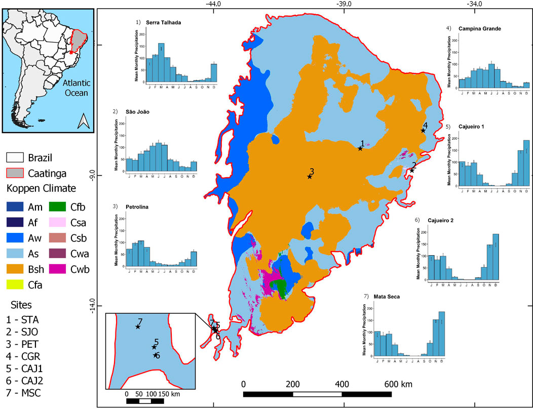
FIGURE 1. Location and climate of the Caatinga in Brazil, delimited by the red line, highlighting the seven study sites (black stars) and Koppen’s climate classification for Brazil from the work of Alvares et al. (2013) with emphasis for the semi-arid (Bsh) climate of Caatinga SDTF in orange. Numbers refer to the location of seven phenocamera study sites: Petrolina (3), Serra Talhada (1), São João (2), Campina Grande (4), Cajueiro 1 (5), Cajueiro 2 (6), and Mata Seca (7) sites. Climate dataset obtained from Abatzoglou et al., 2018 for the period 2000-2020.

TABLE 1

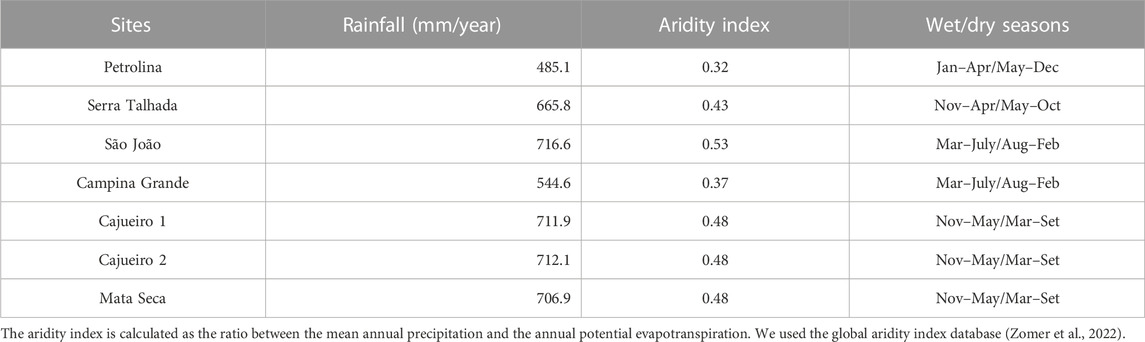
TABLE 1. Mean annual rainfall, aridity index, and the start and end dates of the wet and dry seasons for the Caatinga sites.

2.1.1 Petrolina

It is located at a protected area from the Brazilian Agricultural Research Corporation (Embrapa, semi-arid unit), Petrolina (PET) Municipality (9.0480° S, 40.3198° W), Pernambuco State, at 395 m a.s.l. The area has been protected from grazing and anthropic disturbances for the last 40 years. The most common soil is Acrisol, and the vegetation is a scrubland composed of trees with an average height of ∼4.5 m and tree density of approximately 500 individuals ha⁻¹ over an herbaceous and shrubby stratum dominated by bromeliads. The dominant tree species are Senegalia polyphylla (DC.) Britton and Rose (Fabaceae), Manihot sp. (Euphorbiaceae), Cenostigma microphyllum (Mart. ex G. Don) Gagnon and G.P. Lewis (Fabaceae), Sapium glandulosum (L.) Morong (Euphorbiaceae), Handroanthus spongiosus (Rizzini) S.Grose (Bignoniaceae), and Commiphora leptophloeos (Mart.) J.B.Gillett (Burseraceae). Together, these species account for 88% of the area’s total relative abundance of trees.

2.1.2 Serra Talhada

It is an experimental area located at Serra Talhada (STA) Municipality (7.97008° S; 38.3849° W), Pernambuco State, at 467 m a.s.l. Cattle and goats graze the area during the rainy season. The main soil class is Calcisol, and the vegetation is mainly composed of trees with an average height of ∼5 m and tree density of approximately 780 individuals ha⁻¹. The dominant tree species are Aspidosperma pyrifolium Mart. and Zucc. (Apocynaceae), Cenostigma nordestinum Gagnon and G.P. Lewis (Fabaceae), S. polyphylla, and Anadenanthera colubrina var. cebil (Griseb.) Altschul (Fabaceae). Together, these species account for 79% of the area’s total relative abundance of trees.

2.1.3 São João

It is an experimental area surrounded by agricultural lands located at São João (SJO) Municipality (8.80967°S; 36.4054°W), Pernambuco State, at 762 m a.s.l. Cattle and goats graze the area during the entire year. The most common soil is Arenosol, and the vegetation is mainly composed of trees with an average height of ∼5 m and tree density of approximately 670 individuals ha⁻¹. The dominant tree species are Pilosocereus pachycladus F.Ritter (Cactaceae), C. leptophloeos, Mimosa tenuiflora (Willd.) Poir. (Fabaceae), Piptadenia flava (Spreng. ex DC.) Benth. (Fabaceae), Lippia origanoides Kunth (Verbenaceae), and S. glandulosum. Together, these species account for 71% of the area’s total relative abundance of trees.

2.1.4 Campina Grande

It is a protected area from the Instituto Nacional do Semiárido (INSA) located at Campina Grande (CGA) Municipality (7.280389° S; 35.976307° W), Paraíba State, at 493 m a.s.l. The area has been protected from grazing and anthropic disturbances for the last 10 years. The main soil class is sandy loam, and the vegetation is mainly composed of trees with an average height of ∼5.1 m and tree density of approximately 675 individuals ha⁻¹. The dominant tree species are Cenostigma pyramidale (Tul.) Gagnon and G.P. Lewis (Fabaceae), Combretum monetaria Mart. (Combretaceae), A. pyrifolium, Manihot sp., and P. flava. Together, these species account for 71% of the area’s total relative abundance of trees.

2.1.5 Parque Loagoa do Cajueiro (CAJ 1 and CAJ 2)

It is a conservation area located at Matias Cardoso Municipality, Minas Gerais State, at 462 a.s.l. The mean annual total precipitation is around 712 mm, there are five dry months, and the average annual temperature is 24 °C (Pezzini et al., 2014). There are two distinct vegetation types in the area, and we set up a Mobotix camera in the first and a Bushnell camera in the second. The vegetation in the first area (CAJ 1) is a tall forest composed of trees with an average height of ∼13 m with a closed canopy (∼85%). The dominant tree species are Cenostigma pluviosum var. sanfranciscanum (G.P.Lewis) Gagnon and G.P. Lewis (Fabaceae), A. colubrina (Vell.) Brenan (Fabaceae), Astronium urundeuva M. Allemão (Anacardiaceae), and Plathymenia reticulata Benth. (Fabaceae). The vegetation in the second area (CAJ 2) is an open scrubland SDTF (Carrasco) composed of trees with an average height of ∼4 m with an open canopy (∼30%). The dominant tree species are A. pyrifolium, Callisthene microphylla Warm. (Vochysiaceae), Cenostigma macrophyllum Tul. (Fabaceae), Guapira tomentosa (Casar.) Lundell (Nyctaginaceae), Mimosa arenosa (Willd.) Poir. (Fabaceae), Poecilanthe ulei (Harms) Arroyo and Rudd (Fabaceae), Pterocarpus rohrii Vahl (Fabaceae), Pterodon emarginatus Vogel (Fabaceae), and Terminalia fagifolia Mart. (Combretaceae).

2.1.6 Parque Estadual da Mata Seca

The sixth site is a conservation area located at Manga Municipality, Minas Gerais State, at 462 a.s.l. The area is 3 km from CAJ, the previous site. The mean annual precipitation is 706.9 mm, with five dry season months and 24 °C of mean annual temperature (Pezzini et al., 2014). The vegetation in the area is a tall forest composed of trees with an average height of ∼13 m with a closed canopy (∼95%) and the absence of an herbaceous and shrub layer. The dominant tree species are Handroanthus ochraceus (Cham.) Mattos (Bignoniaceae), Amburana cearensis (Allemão) A.C.Sm. (Fabaceae), A. urundeuva, and Cavanillesia umbellata Ruiz and Pav (Malvaceae).

2.2 Methodology

2.2.1 Camera set up, image acquisition and processing

2.2.1.1 Phenocameras set up and phenological in situ time series

Camera setup: We used images from seven cameras in this study: four digital hemispherical lens MOBOTIX Q25 cameras (MOBOTIX AG, Germany; for detailed information on the usage of MOBOTIX cameras for phenological observations (see Alberton et al., 2017), placed in vertical downward (180°) orientation, and three digital standard lens Bushnell Trophy Cam HD Essential E3 cameras (Bushnell, EUA), placed in landscape orientation (Figure 2). The MOBOTIX cameras were placed on the top of the flux towers in PET (10 m high; Figure 2D), STA (10 m high; Figure 2B), SJO (10 m high; Figure 2C), and at the forest site in CAJ (18 m high; Figure 2F). The MOBOTIX cameras were placed at an average distance of 10 m above the vegetation canopies, positioned to the west (STA and SJO), to the east (PET) and to the northeast (CAJ). The Bushnell cameras were placed at the top of the flux tower in CGA (13 m high; Figure 2E) and Parque Estadual da Mata Seca (MSC) (19 m high; Figure 2H) and on a pole at the Carrasco site in CAJ (6 m high; Figure 2G), positioned to the northwest (CGA) and southwest (MSC and CAJ). The energy supply of Mobotix cameras comes from a system composed of a 12 V battery charged by solar panels, while Bushnell cameras are charged by AA lithium batteries.

FIGURE 2

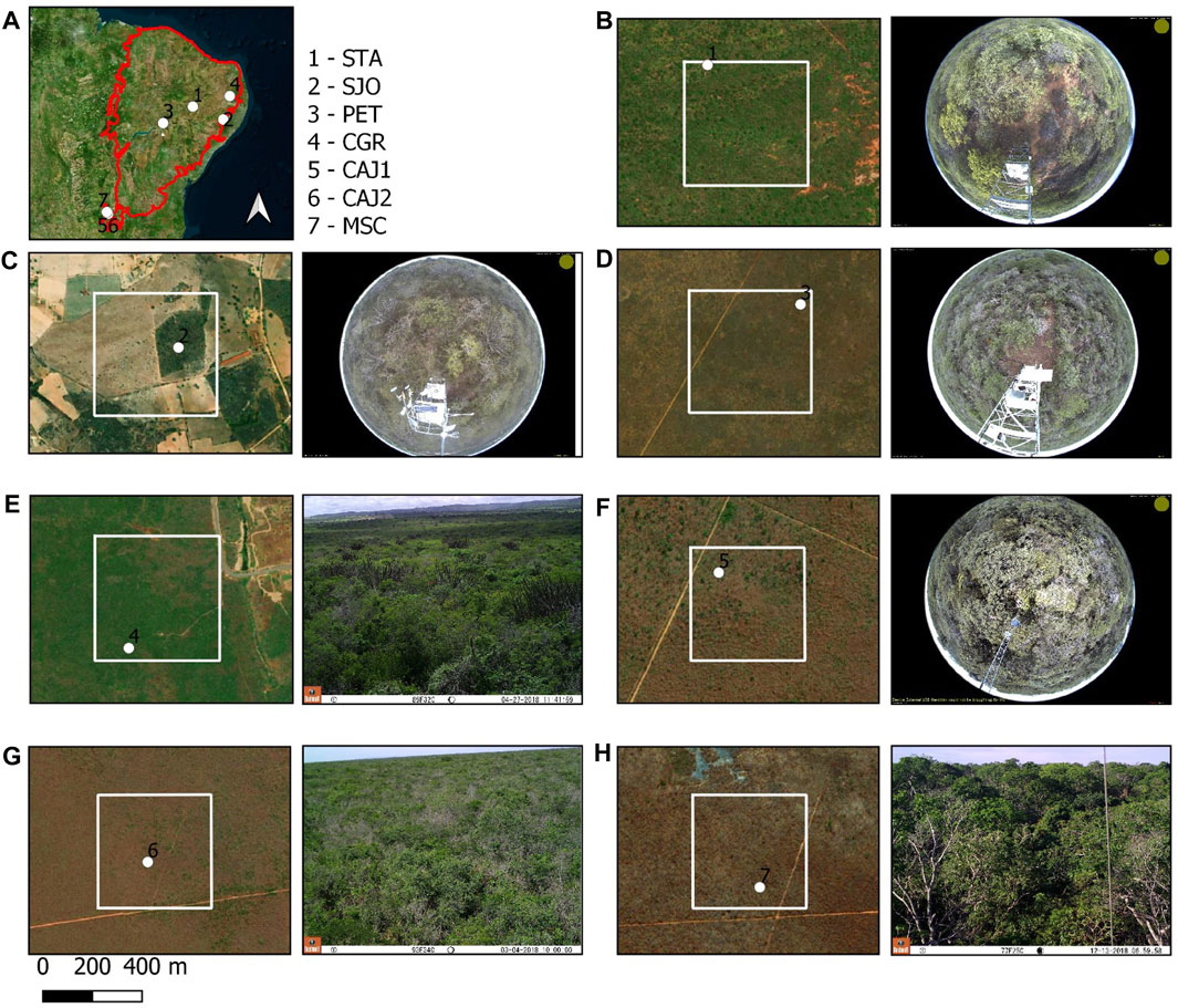
FIGURE 2. General location of the Caatinga study sites. (A) The MODIS pixels (Left), with the phenocamera indicated by the white dot, and the respective typical phenocamera images (right): (B) STA, (C) SJO, (D) PET, (E) CCR, (F) CAJ 1, (G) CAJ 2, and (H) MSC. The globe web-based map was derived from Bing satellite.

Cameras were programmed to take daily images, varying from three to four images, in the first 5 minutes of each hour, from 06:00 a.m. to 06:00 p.m. (UC-3; Universal Time Coordinated). Images were taken in the JPEG format with a pixel resolution of 1,280 × 960 (Alberton et al., 2017). The leafing patterns were registered during one to three growing seasons from 2017 to 2020, with different starting and ending dates depending on the site or camera: PET, 01/11/2017 to 31/12/2020; STA, 28/11/2017 to 31/12/2020; CGA, 28/11/2017 to 31/12/2020; SJO, 20/12/2017 to 03/05/2020, and CAJ, 04/03/2018 to 24/11/2020.

Images were visually screened to remove photographs with an obstructed field of view. To represent the plant community of each site, we drew a region of interest (ROI) in the images, which consisted of the selection of the entire vegetated area but excluded the bare ground, the tower area (for the Mobotix images), and the borders of the image (Alberton et al., 2017; 2019). The digital numbers (DNs) red, green, and blue (RGB) color channels were extracted from the JPEG images for each community ROI across all the daily images available. The total RGB DN was calculated as shown in Eq. 1 (Richardson et al., 2009). Then, the normalized green chromatic coordinate index (GCC; see Alberton et al., 2017; Richardson et al., 2009) was calculated as the ratio of the relative brightness of the green color channel (green DN) to the total DN brightness, as shown in Eq. 2:

$TotalRGBDN=redDN+greenDN+blueDN,(1)$

$Gcc=\frac{GreenDN}{TotalRGBDN}.(2)$

To suppress day-to-day illumination issues in the GCC time series, we calculated the 90th percentile of all mid-day photographs (from 10:00 a.m. to 16:00 p.m.) (adapted from the work of Sonnentag et al., 2012). For data analysis, we used daily GCC time series.

2.2.1.2 Satellite data

The MODIS 16-day nadir BRDF-adjusted reflectance product (MCD43A4) provided the red and near-infrared (NIR) bands for the NDVI calculation. This dataset is produced daily using 16 days of Terra and Aqua MODIS data at 500 m resolution (Guerschman et al., 2015). The landscape had a homogeneous composition in the 500 m resolution pixels used for all the Caatinga sites (Figure 2), except for the SJO site, which was composed mostly of pasture (Figure 2C). Moreover, with the exception of the SJO site, the field of view of phenocamera images was representative of the dominant vegetation observed in the MODIS pixels for all sites (Figure 2).

The images used in this study were from February 2000 to December 2020. The NDVI series were assembled for each experimental site with the pixel value of the MCD43A4 product, the phenocamera being the central pixel of the geographic coordinates of each test site (Figure 2). The processes for obtaining time series NDVI MODIS were performed using the Google Earth Engine (GEE) tool (Gorelick et al., 2017). The GEE tool allows you to visualize, manipulate, edit, and create temporal and spatial data (Gorelick et al., 2017; Li et al., 2017; Pastor-Guzman et al., 2018).

2.3 Data analyses

The workflow to calculate phenological metrics from remote sensing and phenocamera data is described in Figure 3.

FIGURE 3

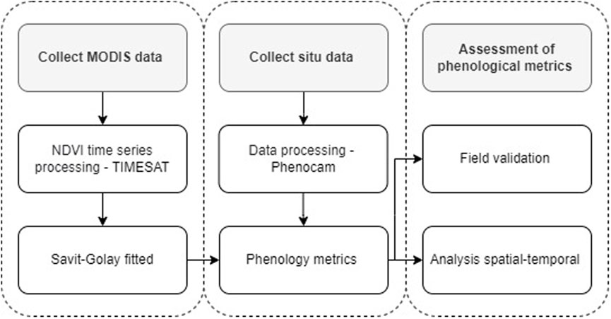
FIGURE 3. Flow chart of the methodology used to calculate the phenological metrics, SOS, EOS, and LOS based on phenocamera in situ and NDVI MODIS time series.

2.3.1 Phenological metrics extracted from the GCC time series

We applied generalized additive models (GAMs) to the camera-derived GCC time series to produce phenological curves (Alberton et al., 2019). Then, we calculated the phenological transition dates (Figure 3) of each growing season by applying the methodology of derivatives proposed by Alberton et al. (2019) and applied in the work of Paloschi et al. (2020). We determined an average threshold value for the GCC greenness rising (50%) for the SOS and green-down (80%) for the EOS. Then, we calculated the length of season (LOS) as the difference between the EOS and SOS dates for each growing season. The SOS corresponds to the start time of the leaf out phenophase, and the EOS the leaf fall phenophase or the time when vegetation is mostly leafless (Alberton et al., 2019; Htitiou et al., 2019). Therefore, the proposed threshold was estimated based on the phenocamera daily photographs to allow visual validation of the phenological transitions of each monitored vegetation site. We used the camera-derived green-up and green-down thresholds to calibrate the extraction of the phenological metrics from the NDVI time series.

2.3.2 Phenological metrics extracted from the NDVI time series

In the initial step, the NDVI time series were calculated in Google Earth Engine (GEE) using near-infrared (NIR) and red bands from MODIS product data (MCD43A4). Next, we used TIMESAT software (Jönsson and Eklundh, 2004; Jönsson and Eklundh, 2012) to smooth the time series and calculated the phenological metrics. The Savitzky–Golay filter (Savitzky and Golay, 1964) from TIMESAT was applied to smooth the NDVI time series. Then, the following phenological metrics were calculated: start of season, end of season, length of season, peak value of NDVI (PEAK), amplitude (AMPL), and the difference between the peak and base level values (see Table 2).

TABLE 2

TABLE 2. Phenological metrics calculated from indices extracted from the phenocamera near-surface phenology (GCC) and from the satellite MODIS land surface phenology (NDVI) indices.

TIMESAT software defines the percentage of the amplitude (threshold) for the vegetation index used. Different amplitude percentages were tested to assess the most appropriate value for all seven sites studied. The phenological metrics derived from the in situ cameras (see Section 2.4.1) were the reference used to evaluate the remote sensing data (i.e., the threshold that corresponds to a given phenocamera transition date). Then, based on the phenocamera thresholds estimated, we set the TIMESAT parameters for estimating the phenological metrics of a 20-year NDVI time series spanning from 2000 to 2019. We calculated the same aforementioned phenological metrics (SOS, EOS, LOS, PEAK, and AMPL) for the twenty-year NDVI time series.

2.4 Statistical analyses

2.4.1 Evaluating remote sensing phenological metrics

To evaluate the better parameters to calculate the remote sensing phenological metrics (SOS and EOS), four amplitudes were tested with different percentiles: 5%, 10%, 15%, and 20%, and compared with the in situ phenological data using the statistical mean absolute error (MAE) (Eq. 3). The thresholds 5%, 10%, 15%, and 20% are commonly used in the literature (Teles et al., 2015; Browning et al., 2017; Ghosh and Mishra, 2017). Moreover, it is necessary to validate the appropriate SOS and EOS thresholds in TIMESAT as these thresholds in tropical dry forests in Brazil have not yet been studied in detail. So, we tested these thresholds to evaluate the best configuration.

$MAE=\frac{1}{n}{\displaystyle \sum _{i=1}^n}\left|y_i-\widehat{y}i\right|,(3)$

where yi represents the value of the in situ phenological metric, ŷi represents the predicted value of remote sensing phenological metric, and n is the number of data (year). After defining the MAE for each site, we computed the mean of MAE values for all sites. The smaller the error, the closer the result of the remote sensing phenological metric to the value of the phenological metric in situ.

2.4.2 Long-term seasonality patterns of the Caatinga and its environmental drivers

To understand the temporal variability of land surface phenology across the Caatinga sites, we used descriptive circular statistics (Zar, 1996; Morellato et al., 2000; Morellato et al., 2010) applied to the phenological metrics SOS, EOS, and peak, calculated from the 20 years’ NDVI time series for each site, separately. We transformed the days of the year (DOYs) into angles of a circumference, resulting in a mean value of ∼1° each day, starting on DOY 1 and stopping on DOY 365 each year (Zar, 1996; Morellato et al., 2010). To describe the temporal patterns of the phenological metrics, we used the mean angle µ, which is the angle around each concentrating most variables. To infer the interannual variability of the phenological metrics across sites, we used the angular standard deviation (±SD) and the concentration (r) around the mean vector.

To evaluate how environmental factors influence land surface phenology across the Caatinga sites, we fitted linear models (lm R function). We examined variation in phenological metrics (length of the growing season (LOS) and productivity (accumulated NDVI and peak of NDVI) as a function of environmental factors using the time series of all sites together. Environmental factors included accumulated precipitation, water deficit, soil moisture, and minimum and maximum temperatures. The environmental factors used in this study were obtained from the TerraClimate database (Abatzoglou et al., 2018) available at GEE. The dataset with a spatial resolution of 0.04° uses climate-assisted interpolation, combining climatological normals from the WorldClim dataset (Abatzoglou et al., 2018), used for various applications (Ahamed et al., 2022; Andrade et al., 2022; Medeiros et al., 2023). We built one linear model for each combination of one response variable and one explanatory variable. We also evaluated if the sites differ in the LOS by fitting a linear model with the LOS as a function of the site since most predictors were highly correlated with each other. We analyzed data in R (R Core Team, 2020).

3 Results

3.1 Phenological patterns from phenocameras and satellite

We recorded phenology simultaneously using phenocameras (GCC) from 2017–2020, which encompassed one to three complete growing seasons, depending on the site (Supplementary Table S1; Figure 4) and overlapping with the MODIS time series (NDVI). The vegetation of all sites showed a seasonal leafing pattern (Figure 4), with marked leaf flushing (GCC and NDVI rising) and leaf fall (GCC and NDVI declining), except for the last growing season (2019–2020) of CAJ 1 registered using a phenocamera, which had 352 days of duration (Supplementary Table S1). For each growing season, the NDVI always peaked after the GCC (Figure 4). The LOS for the Caatinga sites determined using phenocameras was highly variable, ranging from 177 in the driest site, Petrolina, to 352 days in the wettest site, Cajueiro 1, the tallest forest site (Supplementary Table S1). Additionally, there was high interannual variability in the LOS in the three driest sites, ranging from 177 to 245 days, from 216 to 265, and from 229 to 292 in Petrolina, Serra Talhada, and Campina Grande, respectively (Supplementary Table S1).

FIGURE 4

FIGURE 4. Phenocamera GCC (green dots) and MODIS NDVI (orange dots) time series after calibration and the respective phenological transition dates, start of season, and end of season, from 2017 to 2020 for the sites of Petrolina, Campina Grande, Serra Talhada, São João, Cajueiro 1, Cajueiro 2, and Mata Seca. The GCC green dots correspond to the 90th percentiles extracted from the images of the mid-day hours (from 10:00 to 14:00 h), and the NDVI values correspond to the Savitzky–Golay smoothed time series. The vertical lines correspond to the phenological transition dates, SOS (continuous lines), and EOS (dashed lines) calculated for the GCC and NDVI, green and orange lines, respectively.

3.2 Evaluating phenophase transition dates from all platforms

In general, there was good agreement between the SOS calculated from GCC and NDVI time series. The SOS dates for MODIS were biased early by 5 days on average (Supplementary Table S2) in relation to the SOS phenocamera in the lowest MAE selected (5% threshold). The MAE of the SOS dates calculated from the satellite time series in comparison to the camera-derived SOS was highly variable across sites, changing from 6 days at CGA to 53 days at SJO (Table 3). The MAE across sites varied with the threshold used (Table 3), with the 5% threshold resulting in the lowest MAE (14.9 days; Table 3). The usage of the 5% threshold reduced the MAE by 5.27 days compared to the 20% threshold, which is a commonly used value for land surface phenology but produced the highest values of MAE for the Caatinga sites (Table 3).

TABLE 3

TABLE 3. Mean absolute error (MAE) of the start of season estimates varying the values of the estimate and seasonal amplitudes in TIMESAT.

The agreement between the EOS calculated from the GCC and the NDVI time series was worse when compared to the SOS phenophase. The EOS dates for MODIS were biased late by 11 days on average (Supplementary Table S3) in relation to EOS PhenoCam in the lowest MAE selected (20% threshold). The MAE of the EOS dates calculated from the satellite time series in comparison to the camera-derived EOS was highly variable across sites, changing from 9 days at CGA to 99 days at SJO, but was, in general, higher than the MAE for the SOS dates (Table 4). The MAE across sites varied with the threshold used (Table 4), with the 20% threshold resulting in the lowest MAE (25.60 days; Table 4). The usage of the 20% threshold reduced the MAE by 34.34 days compared to the 5% threshold, which produced the highest values of MAE (59.94 days; Table 4). Additionally, usage of the 20% threshold reduced the MAE by 15.60% (Table 4) compared to the 10% threshold, a commonly used value for LSP.

TABLE 4

TABLE 4. Mean absolute error (MAE) of the end of season estimates varying the values of the estimate and seasonal amplitudes in TIMESAT.

3.3 Caatinga leafing patterns from MODIS long-term time series

The transition dates for the start of the season, end of the season, and the NDVI peak of the 20 growing seasons (2000–2019) were seasonal for all seven sites, as indicated by the significance of the Rayleigh test (Z) (Supplementary Table S4). In general, the SD for both TDs and the NDVI peak was lower as the precipitation increased (Figures 5E–F), indicating that the interannual variability in leaf flushing and fall and in the time of the maximum photosynthetic activity decreased toward moist sites. Additionally, the concentration around the mean vector (µ) for these phenophases was low for the driest sites (Figures 5A–C) but increased as the site’s precipitation increased (Figures 5E, F), indicating that the TDs are more concentrated around the mean in the moister sites, which is a characteristic of lower interannual variability. On the other hand, the patterns for the TDs at the SJO site (Figure 5D), which has the highest precipitation among the sites, contrasted with the abovestated result, showing the highest SD and lowest concentration around the mean vector for both TDs and for the time of the NDVI peak.

FIGURE 5

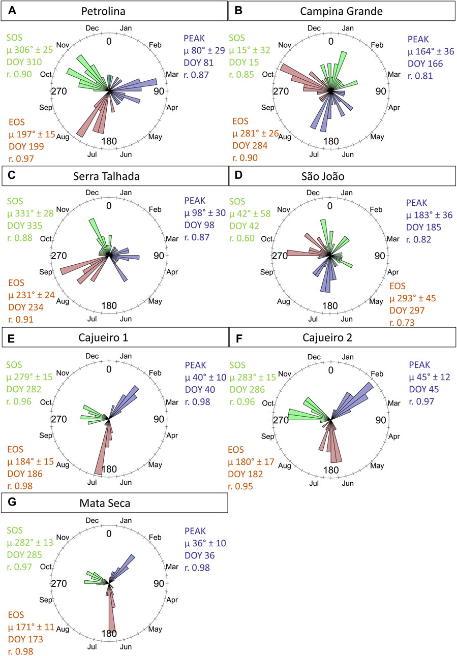
FIGURE 5. Circular histograms of transition dates - TDs representing the Start of Season and the End of Season (SOS and EOS) for the Caatinga sites calculated from MODIS time series from 2000 to 2019. The mean vector (µ) ± SD (standard deviation) for the SOS and EOS is shown in green and brown, respectively. The peak is shown in purple. r = concentration around the mean vector. DOY represents the mean angle converted to day of the year.

The LOS measured with the long-term MODIS time series did not differ on average (F = 1.95; p = 0.07) across the Caatinga sites (Figure 6A) but presented high interannual variability in the driest sites (PET, CGA, STA, and SJO) (PET, CGA, and STA) when compared to the wettest sites (CAJ 1, CAJ 2 and MSC) (Figure 6B), with exception of SJO. This pattern for the LOS confirmed the trend of increasing variability in the LOS for arid sites observed with phenocamera data (Table 3) and added information on the interannual LOS variability for the less arid sites.

FIGURE 6

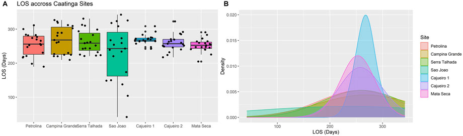
FIGURE 6. Interannual variability of lenght of the season (LOS) for the Caatinga sites calculated from MODIS time series from 2000 to 2019. (A) Mean ± SD and (B) distribution of LOS across sites.

3.4 Caatinga land surface greening patterns from MODIS: long-term time series and environmental drivers

The land surface long-term (from 2000 to 2019) evaluation of the length of the growing season across sites was influenced by the accumulated precipitation but not by water deficit, soil moisture, and minimum and maximum temperatures (Figure 7). The productivity measured as the accumulated NDVI and peak NDVI were influenced by the accumulated precipitation and minimum and maximum temperatures (Figure 7). Thus, a positive relationship was observed between productivity and accumulated precipitation and minimum and maximum temperatures, with increases in productivity when these environmental variables increased (Figure 7).

FIGURE 7

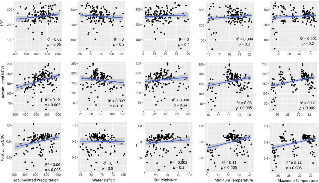
FIGURE 7. Effects of the environmental factors accumulated precipitation, water deficit, soil moisture, and minimum and maximum temperatures on the land surface phenological parameter length of the growing season and the productivity parameters of accumulated NDVI and peak NDVI across the Caatinga sites. Data are long-term land surface NDVI greening extracted from MODIS time series from 2000 to 2019.

4 Discussion

4.1 Seasonal phenological patterns and differences between methods

The GCC and NDVI patterns for all seven sites indicated that the leafing patterns of vegetation were markedly seasonal, a result observed for other seasonally dry ecosystems (Rankine et al., 2017; Yan et al., 2019; Paloschi et al., 2020). The high interannual variability in the LOS registered using phenocams in the driest sites suggests that plants in these communities adjust their phenology to cope with the rainfall unpredictability characteristic of the driest areas in the Caatinga region (de Carvalho et al., 2020). However, this needs to be interpreted with caution for the wettest sites (Cajueiro and Mata Seca) since only one growing season was analyzed.

The peak of GCC always preceded the peak of NDVI for all sites and growing seasons, and this delay may represent two different aspects of the canopy activity. The peak of canopy greenness is sensitive to the changes in the leaf color, representing how green the canopy is, which is influenced by the young leaves being produced (Keenan et al., 2014; Zhang et al., 2018). The NDVI peak is a proxy for the maximum photosynthetic activity (Jin et al., 2013; Del Castillo et al., 2018) and is representative of the total leaf variation on a vegetation canopy (Zhang et al., 2018).

In general, we observed better agreement between the phenocamera- and satellite-derived SOS than for the EOS transition dates. The leaf flushing in the Caatinga SDTF occurs fast and synchronously after the first rains of the rainy season (Alberton et al., 2019; Paloschi et al., 2020), and this pattern was detected similarly in both RS methods. A similar analysis for temperate deciduous vegetation indicates a better correspondence between the SOS and satellite index (Hufkens et al., 2012; Keenan et al., 2014; Klosterman et al., 2014; Zhang et al., 2018) and also for evergreen vegetation (Khare et al., 2022) in those very seasonal ecosystems. The better agreement of TDs from both methods with the SOS is likely related to the fast leaf flushing response in all these markedly seasonal ecosystems (Zhang et al., 2018).

The lower agreement in EOS and the late EOS for the NDVI in comparison to the phenocamera GCC may be caused by the more gradual rate of change of VI from the satellite during leaf fall in comparison to the phenocamera (Hufkens et al., 2012; Yan et al., 2019). However, in the Caatinga SDTF, the phenocamera GCC tends to fall more gradually after its leaf out peak, during the leaf senescence phase, than the NDVI, which may have caused the differences between both methods. Spatial heterogeneity has also been suggested to be an important source of variation in phenological metrics between phenocameras and satellites (Liu et al., 2017; Richardson et al., 2018; Moon et al., 2019), but with the exception of the SJO site in this study, the pixel around the camera used for the satellite NDVI calculations presented a homogenous landscape dominated by the SDTF vegetation (Figure 2). We found that MAE for the SOS and EOS was highest at the SJO site, likely due to the high spatial heterogeneity and the inclusion of sections of farmlands within the pixel encompassing the sampled Caatinga vegetation.

When the calibrated amplitude threshold of 5% for the calculations of the SOS was used, the error between the phenocamera- and satellite-derived SOS was reduced in around 5 days in relation to the 20% threshold, which may not be a significant reduction. However, for the calculation of the EOS phenophase, the usage of the 20% calibrated threshold expressively reduced the error in around 34 days in relation to the 10% threshold. The 20% amplitude threshold for calculating the SOS and EOS transition dates is a common method applied in LSP (Streher et al., 2017; Diem et al., 2018; Doussoulin-Guzmán et al., 2022), but the 10% amplitude threshold suggested by Jönsson and Eklundh (2002) produced lower biases between the phenocamera- and satellite-derived PTs for deciduous broadleaf forests (Richardson et al., 2018) and plants from arid ecosystems (Browning et al., 2017). However, for the semi-arid Caatinga SDTF, the 10% amplitude threshold was shown to produce the highest bias between both methods for the EOS phases, evidencing the importance of understanding the local sources of VI variability and which environmental factors trigger the seasonal responses of the vegetation, to infer trends in LSP.

4.2 Land surface phenological variability across sites and its environmental drivers

The leaf production (SOS) calculated for 20 growing seasons of the NDVI time series from 2000 to 2019 demonstrated, as expected, an increase in the interannual variability towards most arid sites across the Caatinga. The increase in rainfall variability as the total rainfall decreases is a typical characteristic of the Caatinga region, resulting in the unpredictability of rainfall onset and in the mean annual rainfall in these areas across the years (Sampaio, 1995; Gutiérrez et al., 2014; de Carvalho et al., 2020). The leaf flushing of trees generally occurs shortly after the rainfall pulses in the Caatinga vegetation (Machado et al., 1997; Oliveira et al., 2015; Alberton et al., 2019; Paloschi et al., 2020; Alberton et al., 2023; Medeiros et al., 2023), and the higher variability of the SOS in most arid sites indicates a local response of plants to cope with water unpredictability as aridity increases across the Caatinga. A similar result was found for the TDs of brown down or leaf senescence (EOS), with an increase in interannual variability concurrent with increasing aridity. A late or an early EOS can be solely a response to the SOS shifts across years since these phenophases are not uncoupled, with the EOS following the responses of the SOS.

We expected an increase in the length of the growing season with the increase in the mean annual rainfall; however, the LOS did not differ on average across the sites. Also, the land surface parameter length of the growing season (LOS) increased toward the increase in accumulated precipitation, considering the data of all sites and the 20 growing seasons together. Other climatic variables evaluated, such as water deficit, soil moisture, and minimum and maximum temperatures, did not influence the LOS. On the other hand, the interannual variability in LOS was expressively higher with the increase in aridity. These results indicate that although the LOS did not differ across sites, they were adjusted from year to year through the changes in the timings of leaf flush and fall, probably as a response to rainfall variations. The high interannual variability of rainy season duration is likely to favor the coexistence of multiple drought-deciduous strategies inside plant communities, such as evergreen and different levels of deciduousness (Vico et al., 2015).

We measured accumulated and peak NDVI as proxies for ecosystem productivity and found a direct relationship between these variables and water availability (positive relation with accumulated precipitation and soil moisture and negative relation with water deficit). Our results suggest that the Caatinga productivity increases toward the moistest sites and/or when the total annual rainfall is higher. Gross primary productivity (GPP) and evapotranspiration (ET) of Caatinga have demonstrated strong dependency on water availability, being constrained mostly to the rainy season (Costa et al., 2022; Alberton et al., 2023), showing higher productivity in years of higher rainfall (Marques et al., 2020). Nevertheless, it is important to acknowledge that the explained variance in several of the relationships examined between land surface phenology and environmental variables was relatively low. This can likely be attributed to the additive influence of these environmental variables. Even though the relationships were significant for more than one variable, they were tested individually, with one comparison made at a time (for example, accumulated precipitation and peak NDVI and water deficit and peak NDVI), owing to their autocorrelation.

Extreme rainfall events have been observed in the Caatinga region as a consequence of climatic phenomena such as El Niño (Gutiérrez et al., 2014). Additionally, future climate projections for the area indicate rising temperatures, leading to hotter days and nights (Torres et al., 2017). These projections also suggest that surface soils are expected to become drier and more frequent, intense rainfall episodes are expected, followed by prolonged dry and warm periods characterized by a lack of precipitation and extended dry spells (Marengo et al., 2017; Torres et al., 2017). However, it is important to note that climate projections vary across the region (Torres et al., 2017). This emphasizes the critical need for a comprehensive understanding of phenological responses to climate and environmental factors on a larger scale while utilizing the most accurate and precise data available.

5 Conclusion

The phenocamera data successfully improved the accuracy of phenological metrics estimated from satellites, but it was more relevant for the leaf fall (EOS) period than for the leaf flushing (SOS) period. The long-term calibrated satellite phenological measurements unravel the leaf phenological patterns of the Caatinga sites across a large spatial scale. We showed that although all sites share the same semi-arid climate, the phenology of plant communities may be adapted to the changes in local aridity and the predictability of water availability. Aridity shapes land surface phenology across sites, resulting in no differences in averages but increasing the interannual variability in leaf out, fall, and length of the growing season. Additionally, the mean annual rainfall was a good predictor of the growing season length within and across the Caatinga sites.

Data availability statement

The raw data supporting the conclusion of this article will be made available by the authors, without undue reservation.

Author contributions

DR: conceptualization, data curation, formal analysis, investigation, methodology, visualization, writing–original draft, and writing–review and editing. JA: conceptualization, data curation, formal analysis, investigation, methodology, validation, visualization, writing–original draft, and writing–review and editing. BA: conceptualization, data curation, formal analysis, investigation, methodology, visualization, writing–original draft, and writing–review and editing. MM:data curation, funding acquisition, investigation, project administration, and writing–original draft. TD: funding acquisition, project administration, resources, supervision, writing–original draft, and writing–review and editing. NN: data curation, formal analysis, and writing–original draft. JL: data curation, investigation, and writing–review and editing. RS: data curation, investigation, and writing–review and editing. ES: data curation, investigation, project administration, and writing–review and editing. JS: data curation, investigation, and writing–review and editing. ME-S: data curation, investigation, project administration, and writing–review and editing. LM: conceptualization, data curation, funding acquisition, investigation, project administration, resources, supervision, writing–original draft, and writing–review and editing. JC: conceptualization, data curation, formal analysis, funding acquisition, investigation, methodology, project administration, supervision, visualization, writing–original draft, and writing–review and editing.

Funding

The authors declare financial support was received for the research, authorship, and/or publication of this article. This research was funded by the São Paulo Research Foundation FAPESP (grants FAPESP-NERC #2015/50488-5 and FAPESP-Microsoft Research Institute #2013/50155-0, #2009/54208-6, #2019/11835-2, #2021/10639-5, and #2022/07735-5), the National Council for Scientific and Technological Development—CNPq (grants #483223/2011-5 and #409341/2021-5), and FACEPE (Caatinga-FLUX Project, grant APQ 0062-1.07/15). DR and BA received fellowships from FAPESP [(#2017/17380-1) and (#2014/00215-0 and #2016/01413-5), respectively]. LM received research productivity fellowships and grants from CNPq (#311820/2018-2 and #401577/2022-8).

Acknowledgments

The authors thank the Unidade Acadêmica de Serra Talhada (UAST) and Unidade Acadêmica de Garanhuns (UAG) from Universidade Federal Rural de Pernambuco (UFRPE) and the National Observatory of Water and Carbon Dynamics in the Caatinga Biome (NOWCDCB) for allowing the use of academic installations and providing technical assistance and the Instituto Estadual de Florestas de Minas Gerais (IEF-MG) for the support in the Parque Estadual Lagoa do Cajueiro and Parque Estadual da Mata Seca. They also thank Embrapa Semiárido for all the support and collaboration in the Caatinga-FLUX site at Petrolina, Joabe Almeida and Cidney Bezerra for technical support during fieldwork, and Valdemir Silva for support with camera installation.

Conflict of interest

The authors declare that the research was conducted in the absence of any commercial or financial relationships that could be construed as a potential conflict of interest.

Publisher’s note

All claims expressed in this article are solely those of the authors and do not necessarily represent those of their affiliated organizations, or those of the publisher, the editors, and the reviewers. Any product that may be evaluated in this article, or claim that may be made by its manufacturer, is not guaranteed or endorsed by the publisher.

Supplementary material

The Supplementary Material for this article can be found online at: https://www.frontiersin.org/articles/10.3389/fenvs.2023.1275844/full#supplementary-material

References

Abatzoglou, J. T., Dobrowski, S. Z., Parks, S. A., and Hegewisch, K. C. (2018). Terraclimate, a high-resolution global dataset of monthly climate and climatic water balance from 1958-2015. Sci. Data 5, 170191. doi:10.1038/sdata.2017.191

PubMed Abstract | CrossRef Full Text | Google Scholar

Abernethy, K., Bush, E. R., Forget, P., Mendoza, I., and Morellato., L. P. C. (2018). Current issues in tropical phenology: a synthesis. Biotropica 50 (3), 477–482. doi:10.1111/btp.12558

CrossRef Full Text | Google Scholar

Ahamed, A., Knight, R., Alam, S., Pauloo, R., and Melton, F. (2022). Assessing the utility of remote sensing data to accurately estimate changes in groundwater storage. Sci. Total Environ. 807, 150635. doi:10.1016/j.scitotenv.2021.150635

PubMed Abstract | CrossRef Full Text | Google Scholar

Ahlström, A., Raupach, M. R., Schurgers, G., Smith, B., Arneth, A., Jung, M., et al. (2015). The dominant role of semi-arid ecosystems in the trend and variability of the land CO2 sink. Science 348, 895–899. doi:10.1126/science.aaa1668

PubMed Abstract | CrossRef Full Text | Google Scholar

Alberton, B., Almeida, J., Helm, R., Torres, R. S., Menzel, A., and Morellato, L. P. C. (2014). Using phenological cameras to track the green up in a cerrado savanna and its on-the-ground validation. Ecol. Inf. 19, 62–70. doi:10.1016/j.ecoinf.2013.12.011

CrossRef Full Text | Google Scholar

Alberton, B., Martin, T. C. M., Da Rocha, H. R., Richardson, A. D., Moura, M. S. B., Torres, R. S., et al. (2023). Relationship between tropical leaf phenology and ecosystem productivity using phenocameras. Front. Environ. Sci. 11, 1223219. doi:10.3389/fenvs.2023.1223219

CrossRef Full Text | Google Scholar

Alberton, B., Torres, R. D. S., Cancian, L. F., Borges, B. D., Almeida, J., Mariano, G. C., et al. (2017). Introducing digital cameras to monitor plant phenology in the tropics: applications for conservation. Perspect. Ecol. Conservation 15 (2), 82–90. doi:10.1016/j.pecon.2017.06.004

CrossRef Full Text | Google Scholar

Alberton, B., Torres, R. S., Silva, T. S. F., Rocha, H., Soelma, M., and Morellato, P. C. (2019). Leafing patterns and drivers across seasonally dry tropical communities. Remote Sens. 11, 2267. doi:10.3390/rs11192267

CrossRef Full Text | Google Scholar

Alvares, C. A., Stape, J. L., Sentelhas, P. C., Gonçalves, J. L. M., and Sparovek, G. (2013). Köppen’s climate classification map for Brazil. Meteorol. Z. 22 (6), 711–728. doi:10.1127/0941-2948/2013/0507

CrossRef Full Text | Google Scholar

Amorim, I. L. de, Sampaio, E. V. de S. B., and Araújo, E. de L. (2009). Fenologia de espécies lenhosas da caatinga do Seridó, RN. Rev. Árvore 33 (3), 491–499. doi:10.1590/s0100-67622009000300011

CrossRef Full Text | Google Scholar

Andrade, J. M., Neto, A. R., Bezerra, U. A., Moraes, A. C., and Montenegro, S. M. (2022). A comprehensive assessment of precipitation products: temporal and spatial analyses over terrestrial biomes in Northeastern Brazil. Remote Sens. Appl. Soc. Environ. 28, 100842. doi:10.1016/j.rsase.2022.100842

CrossRef Full Text | Google Scholar

Araújo, L. E., Castro, C. C., and de Albuquerque, U. P. (2007). Dynamics of Brazilian Caatinga–a review concerning the plants, environment and people. Funct. Ecosyst. communities 1 (1), 15–28.

Google Scholar

Berra, E. F., and Gaulton, R. (2021). Remote sensing of temperate and boreal forest phenology: a review of progress, challenges and opportunities in the intercomparison of in-situ and satellite phenological metrics. For. Ecol. Manag. 480, 118663. doi:10.1016/j.foreco.2020.118663

CrossRef Full Text | Google Scholar

Browning, D. M., Karl, J. W., Morin, D., Richardson, A. D., and Tweedie, G. E. (2017). Phenocams bridge the gap between field and satellite observations in an arid grassland ecosystem. Remote Sens. 9, 1071. doi:10.3390/rs9101071

CrossRef Full Text | Google Scholar

Caparros-Santiago, J. A., Rodriguez-Galiano, V., and Dash, J. (2021). Land surface phenology as indicator of global terrestrial ecosystem dynamics: a systematic review. ISPRS J. Photogrammetry Remote Sens. 171, 330–347. doi:10.1016/j.isprsjprs.2020.11.019

CrossRef Full Text | Google Scholar

Chambers, L. E., Altwegg, R., Barbraud, C., Barnard, P., Beaumont, L. J., Crawford, R. J. M., et al. (2013). Phenological changes in the southern hemisphere. PLOS ONE 8 (10), e75514. doi:10.1371/journal.pone.0075514

PubMed Abstract | CrossRef Full Text | Google Scholar

Cornelius, C., Estrella, N., Franz, H., and Menzel, A. (2012). Linking altitudinal gradients and temperature responses of plant phenology in the Bavarian Alps. Plant Biol. 15, 57–69. doi:10.1111/j.1438-8677.2012.00577.x

PubMed Abstract | CrossRef Full Text | Google Scholar

Costa, G. B., Mendes, K. R., Viana, L. B., Almeida, G. V., Mutti, P. R., e Silva, C. M. S., et al. (2022). Seasonal ecosystem productivity in a seasonally dry tropical forest (caatinga) using flux tower measurements and remote sensing data. Remote Sens. 14, 3955. doi:10.3390/rs14163955

CrossRef Full Text | Google Scholar

De Beurs, K. M., and Henebry, G. M. (2005). Land surface phenology and temperature variation in the International Geosphere-Biosphere Program high-latitude transects. Glob. Change Biol. 11 (5), 779–790. doi:10.1111/j.1365-2486.2005.00949.x

CrossRef Full Text | Google Scholar

De Beurs, K. M., and Henebry, G. M. (2009). Spatio-temporal statistical methods for modelling land surface phenology. Phenol. Res., 177–208. doi:10.1007/978-90-481-3335-2_9

CrossRef Full Text | Google Scholar

de Carvalho, A. A., Montenegro, A. A. de A., Silva, H. P. da, Lopes, I., Morais, J. E. F. de, and Silva, T. G. F. da. (2020). Trends of rainfall and temperature in Northeast Brazil. Rev. Bras. Eng. Agrícola Ambient. 24 (1), 15–23. doi:10.1590/1807-1929/agriambi.v24n1p15-23

CrossRef Full Text | Google Scholar

Del Castillo, E. G., Sanchez-Azofeifa, A., Gamon, J. A., and Quesada, M. (2018). Integrating proximal broad-band vegetation indices and carbon fluxes to model gross primary productivity in a tropical dry forest. Environ. Res. Lett. 13 (6), 065017. doi:10.1088/1748-9326/aac3f0

CrossRef Full Text | Google Scholar

de Lima, A. L. A., de Sá Barretto Sampaio, E. V., de Castro, C. C., Rodal, M. J. N., Antonino, A. C. D., and de Melo, A. L. (2012). Do the phenology and functional stem attributes of woody species allow for the identification of functional groups in the semiarid region of Brazil? Trees 26 (5), 1605–1616. doi:10.1007/s00468-012-0735-2

CrossRef Full Text | Google Scholar

de Oliveira, C. C., Zandavalli, R. B., de Lima, A. L. A., and Rodal, M. J. N. (2015). Functional groups of woody species in semi-arid regions at low latitudes. Austral Ecol. 40 (1), 40–49. doi:10.1111/aec.12165

CrossRef Full Text | Google Scholar

de Queiroz, L. P., Cardoso, D., Fernandes, M. F., and Moro, M. F. (2017). “Diversity and evolution of flowering plants of the Caatinga domain,” in Caatinga. The largest tropical dry forest region in South America. Editors J. M. da Silva, I. R. Leal, and M. Tabarelli (Germany: Springer International Publishing), 23–63. doi:10.1007/978-3-319-68339-3_2

CrossRef Full Text | Google Scholar

Diem, P., Pimple, U., Sitthi, A., Varnakovida, P., Tanaka, K., Pungkul, S., et al. (2018). Shifts in growing season of tropical deciduous forests as driven by El Niño and La niña during 2001–2016. Forests 9 (8), 448. doi:10.3390/f9080448

CrossRef Full Text | Google Scholar

Doussoulin-Guzmán, M.-A., Pérez-Porras, F.-J., Triviño-Tarradas, P., Ríos-Mesa, A.-F., García-Ferrer Porras, A., and Mesas-Carrascosa, F.-J. (2022). Grassland phenology response to climate conditions in biobio, Chile from 2001 to 2020. Remote Sens. 14 (3), 475. doi:10.3390/rs14030475

CrossRef Full Text | Google Scholar

Fernandes, M. F., Cardoso, D., Pennington, R. T., and de Queiroz, L. P. (2022). The origins and historical assembly of the Brazilian caatinga seasonally dry tropical forests. Front. Ecol. Evol. 10, 1–13. doi:10.3389/fevo.2022.723286

CrossRef Full Text | Google Scholar

Ghosh, S., and Mishra, D. R. (2017). Analyzing the long-term phenological trends of salt marsh ecosystem across coastal Louisiana. Remote Sens. 9 (12), 1340. doi:10.3390/rs9121340

CrossRef Full Text | Google Scholar

Gorelick, N., Hancher, M., Dixon, M., Ilyushchenko, S., Thau, D., and Moore, R. (2017). Google Earth engine: planetary-scale geospatial analysis for everyone. Remote Sens. Environ. 202, 18–27. doi:10.1016/j.rse.2017.06.031

CrossRef Full Text | Google Scholar

Guerschman, J. P., Scarth, P. F., McVicar, T. R., Renzullo, L. J., Malthus, T. J., Stewart, J. B., et al. (2015). Assessing the effects of site heterogeneity and soil properties when unmixing photosynthetic vegetation, non-photosynthetic vegetation and bare soil fractions from Landsat and MODIS data. Remote Sens. Environ. 161, 12–26. doi:10.1016/j.rse.2015.01.021

CrossRef Full Text | Google Scholar

Gutiérrez, A. P. A., Engle, N. L., De Nys, E., Molejón, C., and Martins, E. S. (2014). Drought preparedness in Brazil. Weather Clim. Extrem. 3, 95–106. doi:10.1016/j.wace.2013.12.001

CrossRef Full Text | Google Scholar

Htitiou, A., Boudhar, A., Lebrini, Y., Hadria, R., Lionboui, H., Elmansouri, L., et al. (2019). The performance of random forest classification based on phenological metrics derived from sentinel-2 and landsat 8 to map crop cover in an irrigated semi-arid region. Remote Sens. Earth Syst. Sci. 2, 208–224. doi:10.1007/s41976-019-00023-9

CrossRef Full Text | Google Scholar

Huete, A., Didan, K., Miura, T., Rodriguez, E. P., Gao, X., and Ferreira, L. G. (2002). Overview of the radiometric and biophysical performance of the MODIS vegetation indices. Remote Sens. Environ. 83 (1–2), 195–213. doi:10.1016/S0034-4257(02)00096-2

CrossRef Full Text | Google Scholar

Hufkens, K., Friedl, M., Sonnentag, O., Braswell, B. H., Milliman, T., and Richardson, A. D. (2012). Linking near-surface and satellite remote sensing measurements of deciduous broadleaf forest phenology. Remote Sens. Environ. 117, 307–321. doi:10.1016/j.rse.2011.10.006

CrossRef Full Text | Google Scholar

Jin, C., Xiao, X., Merbold, L., Arneth, A., Veenendaal, E., and Kutsch, W. L. (2013). Phenology and gross primary production of two dominant savanna woodland ecosystems in Southern Africa. Remote Sens. Environ. 135, 189–201. doi:10.1016/j.rse.2013.03.033

CrossRef Full Text | Google Scholar

Jolly, W. M., Nemani, R., and Running, S. W. (2005). A generalized, bioclimatic index to predict foliar phenology in response to climate. Glob. Change Biol. 11 (4), 619–632. doi:10.1111/j.1365-2486.2005.00930.x

CrossRef Full Text | Google Scholar

Jonsson, P., and Eklundh, L. (2002). Seasonality extraction by function fitting to time-series of satellite sensor data. IEEE Trans. Geoscience Remote Sens. 40 (8), 1824–1832. doi:10.1109/tgrs.2002.802519

CrossRef Full Text | Google Scholar

Jönsson, P., and Eklundh, L. (2004). TIMESAT—a program for analyzing time-series of satellite sensor data. Comput. geosciences 30 (8), 833–845. doi:10.1016/j.cageo.2004.05.006

CrossRef Full Text | Google Scholar

Jönsson, P., and Eklundh, L. (2012). Timesat 3.1 - software manual. Lund: Lund University, 82.

Google Scholar

Keenan, T. F., Gray, J., Friedl, M. A., Toomey, M., Bohrer, G., Hollinger, D. Y., et al. (2014). Net carbon uptake has increased through warming-induced changes in temperate forest phenology. Nat. Clim. Chang. 4, 598–604. doi:10.1038/nclimate2253

CrossRef Full Text | Google Scholar

Khare, S., Deslauriers, A., Morin, H., Latifi, H., and Rossi, S. (2022). Comparing time-lapse PhenoCams with satellite observations across the boreal forest of quebec, Canada. Remote Sens. 14, 100. doi:10.3390/rs14010100

CrossRef Full Text | Google Scholar

Klosterman, S. T., Hufkens, K., Gray, J. M., Melaas, E., Sonnentag, O., Lavine, I., et al. (2014). Evaluating remote sensing of deciduous forest phenology at multiple spatial scales using PhenoCam imagery. Biogeosciences 11, 4305–4320. doi:10.5194/bgd-11-2305-2014

CrossRef Full Text | Google Scholar

Li, X., Zhou, Y., Asrar, G. R., and Meng, L. (2017). Characterizing spatiotemporal dynamics in phenology of urban ecosystems based on Landsat data. Sci. Total Environ. 605, 721–734. doi:10.1016/j.scitotenv.2017.06.245

PubMed Abstract | CrossRef Full Text | Google Scholar

Liu, Y., Wang, Z., Sun, Q., Erb, A. M., Li, Z., Schaaf, C. B., et al. (2017). Evaluation of the VIIRS BRDF, Albedo and NBAR products suite and an assessment of continuity with the long term MODIS record. Remote Sens. Environ. 201, 256–274. doi:10.1016/j.rse.2017.09.020

CrossRef Full Text | Google Scholar

Luna-Nieves, A. L., Meave, J. A., Morellato, L. P. C., and Ibarra-Manríquez, G. (2017). Reproductive phenology of useful Seasonally Dry Tropical Forest trees: guiding patterns for seed collection and plant propagation in nurseries. For. Ecol. Manag. 393, 52–62. doi:10.1016/j.foreco.2017.03.014

CrossRef Full Text | Google Scholar

Machado, I. C. S., Barros, L. M., and Sampaio, E. V. S. B. (1997). Phenology of caatinga species at Serra Talhada, PE, northeastern Brazil. Biotropica 29 (1), 57–68. doi:10.1111/j.1744-7429.1997.tb00006.x

CrossRef Full Text | Google Scholar

Marengo, J. A., Torres, R. R., and Alves, L. M. (2017). Drought in Northeast Brazil—past, present, and future. Theor. Appl. Climatol. 129, 1189–1200. doi:10.1007/s00704-016-1840-8

CrossRef Full Text | Google Scholar

Marques, T. V., Mendes, K., Mutti, P., Medeiros, S., Silva, L., Perez-Marin, A., et al. (2020). Environmental and biophysical controls of evapotranspiration from seasonally dry tropical forests (caatinga) in the Brazilian semiarid. Agric. For. Meteorology 287, 107957. doi:10.1016/j.agrformet.2020.107957

CrossRef Full Text | Google Scholar

Medeiros, R., Andrade, J., Ramos, D., Moura, M., Pérez-Marin, A. M., dos Santos, C. A., et al. (2023). Remote sensing phenology of the Brazilian caatinga and its environmental drivers. Remote Sens. 14 (11), 2637. doi:10.3390/rs14112637

CrossRef Full Text | Google Scholar

Melaas, E. K., Sulla-Menashe, D., Gray, J. M., Black, T. A., Morin, T. H., Richardson, A. D., et al. (2016). Multisite analysis of land surface phenology in North American temperate and boreal deciduous forests from Landsat. Remote Sens. Environ. 186, 452–464. doi:10.1016/j.rse.2016.09.014

CrossRef Full Text | Google Scholar

Migliavacca, M., Galvagno, M., Cremonese, E., Rossini, M., Meroni, M., Sonnentag, O., et al. (2011). Using digital repeat photography and eddy covariance data to model grassland phenology and photosynthetic CO2 uptake. Agric. For. Meteorology 151 (10), 1325–1337. doi:10.1016/j.agrformet.2011.05.012

CrossRef Full Text | Google Scholar

Moon, M., Zhang, X., Henebry, G. M., Liu, L., Gray, J. M., Melaas, E. K., et al. (2019). Long-term continuity in land surface phenology measurements: a comparative assessment of the MODIS land cover dynamics and VIIRS land surface phenology products. Remote Sens. Environ. 226, 74–92. doi:10.1016/j.rse.2019.03.034

CrossRef Full Text | Google Scholar

Morellato, L. P. C., Alberti, L. F., and Hudson, I. L. (2010). “Applications of circular statistics in plant phenology: a case studies approach,” in Phenological research. Editors I. L. Hudson, and M. R. Keatley (Dordrecht: Springer Netherlands), 339–359.

CrossRef Full Text | Google Scholar

Morellato, L. P. C., Alberton, B., Alvarado, S. T., Borges, B., Buisson, E., Camargo, M. G. G., et al. (2016). Linking plant phenology to conservation biology. Biol. Conserv. 195, 60–72. doi:10.1016/j.biocon.2015.12.033

CrossRef Full Text | Google Scholar

Morellato, L. P. C., Talora, D. C., Takahasi, A., Bencke, C. C., Romera, E. C., and Zipparro, V. B. (2000). Phenology of Atlantic rain forest trees: a comparative study. Biotropica 32, 811–823. doi:10.1111/j.1744-7429.2000.tb00620.x

CrossRef Full Text | Google Scholar

Paloschi, R. A., Ramos, D. M., Ventura, D. J., Souza, R., Souza, E., Morellato, L. P. C., et al. (2020). Environmental drivers of water use for caatinga woody plant species: combining remote sensing phenology and sap flow measurements. Remote Sens. 13 (1), 75. doi:10.3390/rs13010075

CrossRef Full Text | Google Scholar

Pastor-Guzman, J., Dash, J., and Atkinson, P. M. (2018). Remote sensing of mangrove forest phenology and its environmental drivers. Remote Sens. Environ. 205, 71–84. doi:10.1016/j.rse.2017.11.009

CrossRef Full Text | Google Scholar

Pezzini, F. F., Ranieri, B. D., Brandão, D. O., Fernandes, G. W., Quesada, M., Espírito-Santo, M. M., et al. (2014). Changes in tree phenology along natural regeneration in a seasonally dry tropical forest. Plant Biosyst. 148 (5), 965–974. doi:10.1080/11263504.2013.877530

CrossRef Full Text | Google Scholar

Piao, S., Liu, Q., Chen, A., Janssens, I. A., Fu, Y., Dai, J., et al. (2019). Plant phenology and global climate change: current progresses and challenges. Glob. Change Biol. 25 (6), 1922–1940. doi:10.1111/gcb.14619

PubMed Abstract | CrossRef Full Text | Google Scholar

Polgar, C. A., and Primack, R. B. (2011). Leaf-out phenology of temperate woody plants: from trees to ecosystems. New Phytol. 191 (4), 926–941. doi:10.1111/j.1469-8137.2011.03803.x

PubMed Abstract | CrossRef Full Text | Google Scholar

Rankine, C., Sánchez-Azofeifa, G. A., Guzmán, J. A., Espirito-Santo, M. M., and Sharp, I. (2017). Comparing MODIS and near-surface vegetation indexes for monitoring tropical dry forest phenology along a successional gradient using optical phenology towers. Environ. Res. Lett. 12 (10), 105007. doi:10.1088/1748-9326/aa838c

CrossRef Full Text | Google Scholar

R Core Team (2020). R: a language and environment for statistical computing. Vienna, Austria: R Foundation for Statistical Computing. Available at: http://www.R-project.org/ December 10, 2020).

Google Scholar

Reich, P. B. (1995). Phenology of tropical forests: patterns, causes, and consequences. Can. J. Bot. 73, 164–174. doi:10.1139/b95-020

CrossRef Full Text | Google Scholar

Ribeiro, E. M. S., Arroyo-Rodríguez, V., Santos, B. A., Tabarelli, M., and Leal, I. R. (2015). Chronic anthropogenic disturbance drives the biological impoverishment of the Brazilian Caatinga vegetation. J. Appl. Ecol. 52, 611–620. doi:10.1111/1365-2664.12420

CrossRef Full Text | Google Scholar

Richardson, A. D., Andy Black, T., Ciais, P., Delbart, N., Friedl, M. A., Gobron, N., et al. (2010). Influence of spring and autumn phenological transitions on forest ecosystem productivity. Philosophical Trans. R. Soc. B Biol. Sci. 365 (1555), 3227–3246. doi:10.1098/rstb.2010.0102

PubMed Abstract | CrossRef Full Text | Google Scholar

Richardson, A. D., Braswell, B. H., Hollinger, D. Y., Jenkins, J. P., and Ollinger, S. V. (2009). Near-surface remote sensing of spatial and temporal variation in canopy phenology. Ecol. Appl. 19, 1417–1428. doi:10.1890/08-2022.1

PubMed Abstract | CrossRef Full Text | Google Scholar

Richardson, A. D., Hufkens, K., Milliman, T., and Frolking, S. (2018). Intercomparison of phenological transition dates derived from the PhenoCam Dataset V1.0 and MODIS satellite remote sensing. Sci. Rep. 8 (1), 5679. doi:10.1038/s41598-018-23804-6

PubMed Abstract | CrossRef Full Text | Google Scholar

Richardson, A. D., Jenkins, J. P., Braswell, B. H., Hollinger, D. Y., Ollinger, S. V., and Smith, M. L. (2007). Use of digital webcam images to track spring green-up in a deciduous broadleaf forest. Oecologia 152 (2), 323–334. doi:10.1007/s00442-006-0657-z

PubMed Abstract | CrossRef Full Text | Google Scholar

Richardson, A. D., Keenan, T. F., Migliavacca, M., Ryu, Y., Sonnentag, O., and Toomey, M. (2013). Climate change, phenology, and phenological control of vegetation feedbacks to the climate system. Agric. For. Meteorol. 169, 156–173. doi:10.1016/j.agrformet.2012.09.012

CrossRef Full Text | Google Scholar

Sampaio, E. (1995). “Overview of the Brazilian caatinga,” in Seasonally dry tropical forests. Editors S. H. Bullock, H. A. Mooney, and E. Medina (New York: Cambridge University Press), 35–58.

CrossRef Full Text | Google Scholar

Savitzky, A., and Golay, M. J. E. (1964). Smoothing and differentiation of data by simplified least squares procedures. Anal. Chem. 36 (8), 1627–1639. doi:10.1021/ac60214a047

CrossRef Full Text | Google Scholar

Silva, J. O., Espírito-Santo, M. M., Santos, J. C., and Rodrigues, P. (2020). Does leaf flushing in the dry season affect leaf traits and herbivory in a tropical dry forest? Sci. Nat. 107 (6), 51–10. doi:10.1007/s00114-020-01711-z

PubMed Abstract | CrossRef Full Text | Google Scholar

Sonnentag, O., Hufkens, K., Teshera-Sterne, C., Young, A. M., Friedl, M., Braswell, B. H., et al. (2012). Digital repeat photography for phenological research in forest ecosystems. Agric. For. Meteorol. 22, 159–177. doi:10.1016/j.agrformet.2011.09.009

CrossRef Full Text | Google Scholar

Souza, R., Feng, X., Antonino, A., Montenegro, S., Souza, E., and Porporato, A. (2016). Vegetation response to rainfall seasonality and interannual variability in tropical dry forests. Hydrol. Process. 30 (20), 3583–3595. doi:10.1002/hyp.10953

CrossRef Full Text | Google Scholar

Streher, A. S., Sobreiro, J. F. F., Morellato, L. P. C., and Silva, T. S. F. (2017). Land surface phenology in the tropics: the role of climate and topography in a snow-free mountain. Ecosystems 20 (8), 1436–1453. doi:10.1007/s10021-017-0123-2

CrossRef Full Text | Google Scholar

Teles, T. S., Galvão, L. S., Breunig, F. M., Balbinot, R., and Gaida, W. (2015). Relationships between MODIS phenological metrics, topographic shade, and anomalous temperature patterns in seasonal deciduous forests of south Brazil. Int. J. Remote Sens. 36 (18), 4501–4518. doi:10.1080/01431161.2015.1084437

CrossRef Full Text | Google Scholar

Thapa, S., Garcia Millan, V. E., and Eklundh, L. (2021). Assessing forest phenology: a multi-scale comparison of near-surface (uav, spectral reflectance sensor, PhenoCam) and satellite (MODIS, sentinel-2) remote sensing. Remote Sens. 13, 1597. doi:10.3390/rs13081597

CrossRef Full Text | Google Scholar

Torres, R. R., Lapola, D. M., and Gamarra, N. R. L. (2017). “Future climate change in the Caatinga,” in Caatinga. The largest Tropical dry forest region in South America. Editors J. M. C. Silva, I. R. Leal, and M. Tabarelli (Cham: Springer International Publishing), 383–409.

CrossRef Full Text | Google Scholar

Tuanmu, M.-N., Viña, A., Bearer, S., Xu, W., Ouyang, Z., Zhang, H., et al. (2010). Mapping understory vegetation using phenological characteristics derived from remotely sensed data. Remote Sens. Environ. 114 (8), 1833–1844. doi:10.1016/j.rse.2010.03.008

CrossRef Full Text | Google Scholar

Vico, G., Thompson, S. E., Manzoni, S., Molini, A., Albertson, J. D., Almeida-Cortez, J. S., et al. (2015). Climatic, ecophysiological, and phenological controls on plant ecohydrological strategies in seasonally dry ecosystems. Ecohydrology 8 (4), 660–681. doi:10.1002/eco.1533

CrossRef Full Text | Google Scholar

Wang, J., Song, G., Liddell, M., Morellato, P., Lee, C. K. F., Yang, D., et al. (2023). An ecologically-constrained deep learning model for tropical leaf phenology monitoring using PlanetScope satellites. Remote Sens. Environ. 286, 113429. doi:10.1016/j.rse.2022.113429

CrossRef Full Text | Google Scholar

Wright, C. L., Lima, A. L. A., Souza, E. S., West, J. B., and Wilcox, B. P. (2021). Plant functional types broadly describe water use strategies in the Caatinga, a seasonally dry tropical forest in northeast Brazil. Ecol. Evol. 11 (17), 11808–11825. doi:10.1002/ece3.7949

PubMed Abstract | CrossRef Full Text | Google Scholar

Yan, D., Scott, R. L., Moore, D. J. P., Biederman, J. A., and Smith, W. K. (2019). Understanding the relationship between vegetation greenness and productivity across dryland ecosystems through the integration of PhenoCam, satellite, and eddy covariance data. Remote Sens. Environ. 223, 50–62. doi:10.1016/j.rse.2018.12.029

CrossRef Full Text | Google Scholar

Zar, J. H. (1996). Biostatistical analysis. Upper Saddle River, New Jersey: Prentice-Hall, 662.

Google Scholar

Zeng, L., Wardlow, B. D., Xiang, D., Hu, S., and Li, D. (2020). A review of vegetation phenological metrics extraction using time-series, multispectral satellite data. Remote Sens. Environ. 237, 111511. doi:10.1016/j.rse.2019.111511

CrossRef Full Text | Google Scholar

Zhang, X., Friedl, M. A., Schaaf, C. B., Strahler, A. H., Hodges, J. C. F., Gao, F., et al. (2003). Monitoring vegetation phenology using MODIS. Remote Sens. Environ. 84, 471–475. doi:10.1016/S0034-4257(02)00135-9

CrossRef Full Text | Google Scholar

Zhang, X., Jayavelu, S., Liu, L., Friedl, M. A., Henebry, G. M., Liu, Y., et al. (2018). Evaluation of land surface phenology from VIIRS data using time series of PhenoCam imagery. Agric. For. Meteorology 256-257, 137–149. doi:10.1016/j.agrformet.2018.03.003

CrossRef Full Text | Google Scholar

Zomer, R. J., Xu, J., and Trabucco, A. (2022). Version 3 of the global aridity index and potential evapotranspiration database. Sci. Data 9 (1), 409. doi:10.1038/s41597-022-01493-1

PubMed Abstract | CrossRef Full Text | Google Scholar