Evolution characteristics, carbon emission effects and influencing factors of production-living-ecological space in Taihang Mountain poverty belt, China

The rapid advancement of urbanization and industrialization in China has gradually spread to the poor mountainous areas, which has not only brought about rapid economic development but has also caused the increasing competition for production-living-ecological spaces (PLES) and many ecological and environmental problems, carbon emissions have also increased. As an economically less developed and ecologically fragile area in China, whether the transition of the PLES in the mountain poverty belt has unique characteristics? How the PLES transition in mountainous areas affects carbon emissions and what are the important factors affecting carbon emissions? To explore these issues in depth, we studied the Taihang Mountain area in Shijiazhuang (TMS) using remote sensing image interpretation data from 2000, 2010, and 2020, and we analyzed the PLES evolution characteristics, carbon emission changes, carbon emission effects and its influencing factors of PLES. The results are as follows: 1) The TMS was dominated by ecological and production space. From 2000 to 2020, the production space decreased by 384.66 km², the ecological space increased by 123.80 km², and the living space increased by 260.86 km². Agricultural production space was mainly converted to ecological and rural living space. Industrial and mining productive space was mainly converted to agricultural productive space and urban living space. 2) The study area was in a state of carbon deficit, the transition of ecological space and agricultural productive space to industrial and mining productive space and living space were the main transition types caused the carbon emissions increasing, and that of industrial and mining productive space to agricultural productive space was the main type caused the carbon emissions decreasing. 3) The proportion of construction land, urbanization rate and proportion of secondary industry are the main factors leading to the increase of carbon emissions. Per capita energy consumption, forest coverage and proportion of tertiary industry are the main factors leading to the decrease of carbon emissions. This can provide new ideas for research on carbon emissions from land-use changes and a theoretical basis for the optimization of territorial space in the mountainous areas of China.

1 Introduction

Recently, China has made significant progress in its economic development. Simultaneously, rapid urbanization and industrialization have led to man–land and production–living–ecological spaces (PLES) conflicts, which have caused many ecological and environmental problems, including rapid increases in carbon emissions. The carbon emissions of China account for about 25% of the global total (Zhou, et al., 2023). The Chinese government has been committed to achieve carbon peak and carbon neutrality by 2030 and 2060. With the implementation of Chinese territorial spatial planning, the priority of China’s land management strategy has shifted from land-use patterns to space regulation, that is, the PLES mode (Zhang et al., 2021). PLES transition is a deepening application of land-use transition in the new era. Many studies have shown that land-use transition is an important cause of carbon emissions (Houghton, 2018). It is unknown how the PLES transition affect carbon emissions. Mountainous areas in China are economically less developed and ecologically fragile, as well as important ecological environment protection areas and carbon sink sources. Recently, these areas have faced the dual tasks of economic development and ecological protection, causing a complicated land-use transition (Zhang et al., 2018) and the conflict of PLES, which has induced a series of social, economic, and ecological effects. Therefore, it is important to study PLES transition and its carbon emission effect.

Land use is a hotspot issue facing mankind (Arrow, et al., 1995), and many studies have been carried out on the issue, focusing on land-use transitions (Drummond et al., 2017), land use/cover changes (LUCCs) (Goldewijk, 2001; Winkler et al., 2021), the effects of land use/cover changes on biodiversity (Newbold et al., 2015), ecosystem services (Balthazar et al., 2014), greenhouse gases (de Sousa-Neto et al., 2018), nitrogen (Ojoyi et al., 2017), and the influencing factors of land use change (Weber et al., 2001; Deslatte et al., 2022; Lambin et al., 2011). With the introduction of PLES in China and its gradual evolution into an important theoretical direction land use, many studies have been conducted under the framework of PLES, such as the functional identification and spatial division (Duan et al., 2021; Bai et al., 2022), coupling coordination analysis (Yang et al., 2020; Cui et al., 2022), spatial conflict (Zhao et al., 2022), and spatial pattern optimization (Tian et al., 2020; Liao et al., 2022).Among them, research on the transition of PLES and ecological effects is currently a very important research aspect, involving research on ecosystem service value (Wang et al., 2022), eco-environment quality (Yang et al., 2018), and study areas covering China (Kong et al., 2021), provinces (Chen et al., 2022), and cities (Jiang et al., 2022). As an economically less developed and ecologically fragile area in China, it is worth studying further whether the transition of the PLES in the mountain poverty belt has unique characteristics.

Land-use change is one of the most important causes of carbon emissions. The net carbon emissions from land-use changes accounted for 12.5% of total carbon emissions in the world from 1990 to 2010 (Houghton et al., 2012). About 1/4 of anthropogenic carbon emissions were caused by land-use changes over the past 20 years (Barnett et al., 2005). In tropical Asia, carbon emissions from land-use change accounted for approximately 75% of total carbon emissions (Houghton and Hackler, 1999). Land use changes may emit tens of billions of tons of carbon over the next few centuries (Schimel, 2010). How does PLES transition affect China’s carbon emissions? Some researchers pointed out that the spatial evolution of PLES has a negative impact on carbon emissions (Liu et al., 2023). Some researchers pointed out that the expansion of living space leads to an increase in carbon emissions (Li et al., 2023), and some researchers believed that the transition of ecological space to production and living spaces was the main reason for the increase in carbon emissions (Zheng et al., 2022). Mountainous areas in China are important carbon sink sources and play a vital role in protecting the regional ecological environment and reducing carbon emissions. Therefore, the manner in which the PLES transition in mountainous areas affects regional carbon emissions requires further study.

Influencing factors of carbon emissions is another significant research direction of carbon emissions. Many studies point out that economics, population, technology, industrial structures, and energy structures significantly affect carbon emissions (Ang et al., 1998; Chontanawat, 2018; Vujovi et al., 2018). Generally, economic increase and population growth caused the increasing of energy demand, therefore resulting in increased carbon emissions (Henriques and Borowiecki, 2017; Li, 2020). It shows an inverted U-shaped relationship between economic development and carbon emissions (Hidemichi et al., 2018; Arshed et al., 2021). Technological progress and industrial structure optimization are helpful to decreasing carbon emissions (Wang, et al., 2018). Urbanization is also an important reason in regard to the increase in carbon emissions in Asian countries (Shahbaz et al., 2015; Nosheen et al., 2020). Afforestation increases carbon sinks, whereas deforestation increases carbon emissions (Woodbury et al., 2007). Whether the transition of the PLES has a direct impact on carbon emissions requires further investigation. What are the important factors affecting carbon emissions in mountainous areas? It should be noted though that there are few studies on special regions, especially mountain poverty belts.

Based on this, this study takes the Taihang Mountains area of Shijiazhuang (TMS) in China as an example, aimed to deeply analyze the carbon emission effects of the PLES and examine the influencing factors on carbon emissions. The indicators of “Contribution rate of PLES transition to carbon emissions” and “Marginal carbon emissions of PLES” were introduced to describe the carbon emission effects, and the Improved STIRPAT Model was used to examine the influencing factors on carbon emissions. Theoretically, this study can provide new ideas for international research on land-use change and carbon emissions, and enrich international research on the factors influencing carbon emissions. Practically, the results of this study can provide a theoretical basis for the optimization of land space and low-carbon development in mountainous areas of China and provide a reference for the formulation of relevant land space control policies.

According to the purpose, the remaining elements of the paper is arranged as follows. The Materials and Methods are organized in Section 2, and Section 3 is Results analysis. The final Section 4 concludes Discussion, Conclusion and the Policy suggestions.

2 Materials and methods

2.1 Study area

The Taihang Mountain area in the west of Shijiazhuang (TMS) is located in the middle of the Taihang Mountain area in Hebei Province (Figure 1) between 37° 27′-38° 42′N and 113° 31′- 114° 33′E, and it includes Xingtang County, Lingshou County, Pingshan County, Jingxing Mining Area, Luquan District, Jingxing County, Yuanshi County, and Zanhuang County. The terrain of the TMS is high in the west and low in the east, with an altitude of 100–2281 m. The geomorphic types vary and are complicated; there are mid-mountains, low mountains, hills, intermountain basins, and valleys from east to west. The study area is ecologically fragile. The land use pattern has undergone urban expansion, reduction in cultivated land, deforestation to cultivated land abandonment, and recovery growth of forest land. It is the epitome of the transition of PLES in mountainous areas of China.

Figure 1

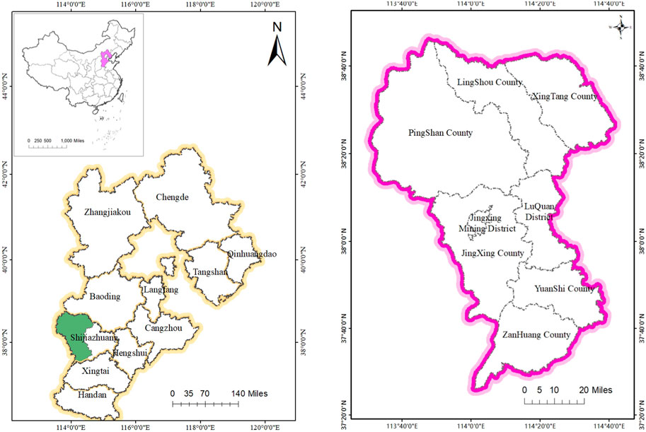
Figure 1. The geographical location of TMS.

2.2 Data sources

Land use data (30 m resolution) from 2000, 2010, and 2020 were obtained from the Data Centre for Resources and Environmental Sciences, Chinese Academy of Sciences (https://www.resdc.cn). Socio-economic data and energy data were obtained from the “Shijiazhuang Economic Statistics Yearbook,” and soil data from the second national soil survey of Hebei Province.

About the division of PLES, land use types were divided into single functional types (Chen et al., 2015) and composite functional types (Zhang et al., 2017). Based on the classification criteria (Data Center for Resources and Environmental Sciences, 2018), this paper classifies PLES into 3 primary categories, that is Production space (PS), Living space (LS), Ecological space (ES); and 8 subcategories, that is Agricultural productive space (APS), Industrial and mining productive space (IMPS), Urban living space (ULS), Rural living space (RLS), Forest ecological space (FES), Meadow ecological space (MES), Water ecological space (WES) and Other ecological space (OES).

2.3 Methods

2.3.1 Transfer matrix of PLES

The transfer matrix of PLES can not only disclose the PLES structure but also quantitatively describe the dynamic evolution of PLES transition from the beginning to the end. The transfer matrixes of 2000–2010, 2010–2020, and 2000–2020 were obtained using the spatial overlay function of ArcGIS. As shown in Formula 1:

$S_{ij}=\left[\begin{array}{cccc}{S}_{11}& S_{12}& ...& S_{1n}\\ S_{21}& S_{22}& ...& S_{2n}\\ ...& ...& ...& ...\\ S_{m1}& S_{m2}& ...& S_{mn}\end{array}\right](1)$

where S is the area of PLES and S_ij is the area transferred from type i to type j. Each row in the matrix represents the flow direction from type i to other types, and each column represents the source from other types to type j. The transfer-in and transfer-out areas of PLES were calculated based on the transfer matrix, and the percentage of the transferred area was calculated based on PLES in different periods.

2.3.2 Carbon emission calculation of PLES

2.3.2.1 Calculation of carbon emissions

Carbon emissions are calculated by carbon density and corresponding land use area, the expression is as follows:

$C_s={\displaystyle \sum _{i=1}^n}{S}_{\mathrm{i}}*S{D}_i(2)$

where C_s is total carbon emission, S_i is the area of PLES, i = 1,2. n represents the type of PLES, SD_i is carbon density, where “−”represents carbon sink, “+” represents carbon emission.

Referring to the carbon density of different land use types by relevant research (Zhu et al., 2019; Yang et al., 2020), we constructed the preliminary carbon density of PLES in the TMS. On this basis, we modified the soil carbon sink density referring to the soil carbon density of each soil type in Hebei Plain (Luan et al., 2011; Gao et al., 2018). The vegetation carbon sink density was modified based on the carbon density of different vegetation types in North China (Chen, 2003). Furthermore, the carbon emissions density was modified referring to the corresponding relationship between industrial space and energy consumption (Zhao et al., 2010). Finally, we determined the carbon density of PLES in the TMS (Table 1).

Table 1

Table 1. Carbon density of production—living–ecological spaces (PLES) Unit: t/hm².

2.3.2.2 Contribution rate of PLES transition to carbon emissions

Referring to the index of “ecological contribution rate of land use transition (Yang et al., 2018),” we introduce the index of carbon-emissions contribution rate of PLES transition as follows:

$\mathrm{R}=\left({\mathrm{C}}_{\mathrm{b}}-{\mathrm{C}}_{\mathrm{e}}\right){\mathrm{S}}_{\mathrm{i}}/\Delta \text{TC}(3)$

where R is the carbon-emissions contribution rate of the PLES transition, C_b is the carbon density in the beginning, C_e is the carbon density in the end, S_i is the area of PLES transition, and ΔTC is the carbon emission changes during the period.

2.3.2.3 Marginal carbon emissions of PLES

Marginal carbon emissions is the change in carbon emissions caused by the change of per unit PLES, which indicates the sensitivity of the area to carbon emissions (Hu et al., 2015). The expression is as follows:

$\text{MC}=\text{TC}/\mathrm{S}(4)$

where MC is the marginal carbon emissions, TC is carbon emission changes, and S is area changes.

2.3.3 Analysis of influencing factors of carbon emissions

2.3.3.1 Improved STIRPAT model

The STIRPAT model was firstly proposed by York and Dietz (York et al., 2003) based on the IPAT identity, and it has been applied widely to examine the influence of population, economy and technology on ecological environment. It also been used to estimate the influencing factors of CO₂ emissions and has good scalability. The basic expression is as follows:

$I=a{P}^b{A}^c{T}^{d}e(5)$

where I represents the environmental effect, P represents the population, A represents the wealth, T represents technology; a is the dominant coefficient; b, c, and d are Elasticity coefficients; and e is error.

We take the logarithm of the two sides and construct an extended influencing factors, then get Model (6):

$\ln I=\ln a+b\ln P+c\ln A+d\ln T+\ln e+f\ln O(6)$

where I represents CO₂ emissions, lna is a constant term, lne is a random distractor, O is added factor.

2.3.3.2 Variable description

Based on the research of carbon emissions caused by land use changes (Fahey et al., 2010; Zhang et al., 2021), the land use changes of forest land and construction land will cause carbon emission changes, therefore, the paper added the indicators of forest coverage rate and proportion of construction land. As shown in Table.2.

Table 2

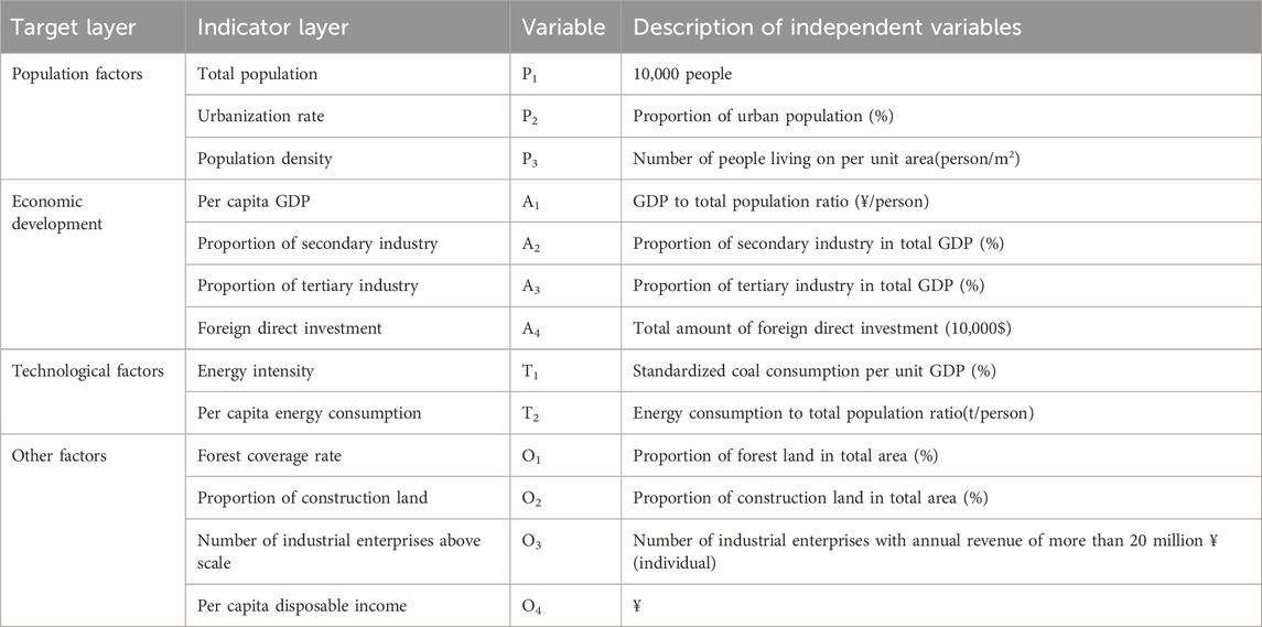
Table 2. Indicator of carbon emission influencing.

3 Results

3.1 Evolution characteristics of PLES

PLES in the TMS is dominated by ecological space and production space, of which agricultural productive space accounts for the largest proportion, next came forest ecological space and grassland ecological space; the sum of these three spaces accounts for more than 90% in the TMS. The evolution characteristics of PLES are: 1) From 2000 to 2020, the production space decreased by 384.66 km², of which agricultural productive space decreased continuously by a total of 380.19 km². Industrial and mining productive space first increased by 8.60 km² from 2000 to 2010 and then decreased by 13.07 km² from 2010 to 2020. 2) From 2000 to 2020, ecological space increased slightly by 123.80 km², of which forest ecological space first increased by 247.22 km² from 2000 to 2010 and then decreased by 105.99 km² from 2010 to 2020. Meadow ecological space first decreased by 111.54 km² from 2000 to 2010 and then increased by 116.18 km² from 2010 to 2020. 3) From 2000 to 2020, living space significantly increased by 260.86 km². Urban and rural living spaces increased continuously by 71.28 km² and 189.58 km², respectively (Table 3).

Table 3

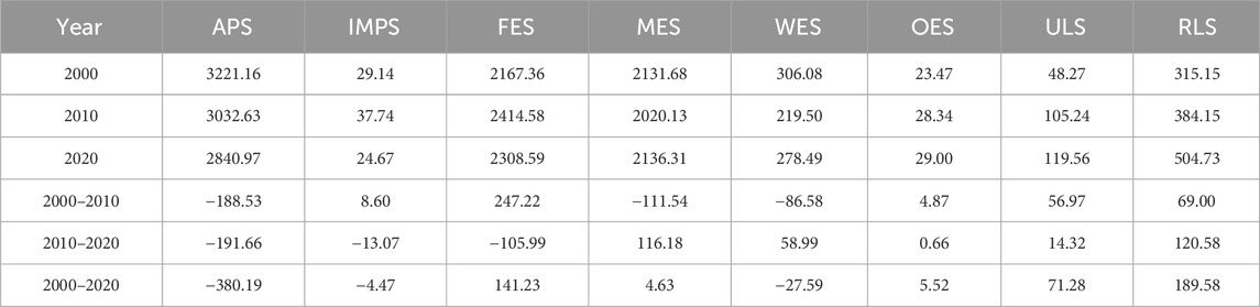
Table 3. Areas and changes in PLES of the TMS during 2000-2020. Unit: km².

With the rapid economic development and urbanization of Shijiazhuang City, urban and rural living spaces increased rapidly. Also, agricultural productive space was occupied, leading to serious contradictions between living and production land. Recently, with the reformation of the energy structure, high-energy-consumption, high-pollution, and high-emissions industries were eliminated, and the growth in industrial and mining productive space was controlled.

As shown in Figure 2, forest and meadow ecological spaces are mainly distributed in Pingshan, Jingxing, Lingshou, and Zanhuang County. Water ecological space includes Hutuo River, Gangnan Reservoir, and Huangbizhuang Reservoir, which are located in Pingshan County and Luquan District. Agricultural productive space is mainly located in the east of TMS, such as Xingtang, Luquan, and Yuanshi County. Urban living space is scattered in each county (district) and is concentrated in Luquan District and Jingxing Mining District. Industrial productive space is generally located in the peripheral areas of urban living space, while rural living space is scattered in all counties (districts).

Figure 2

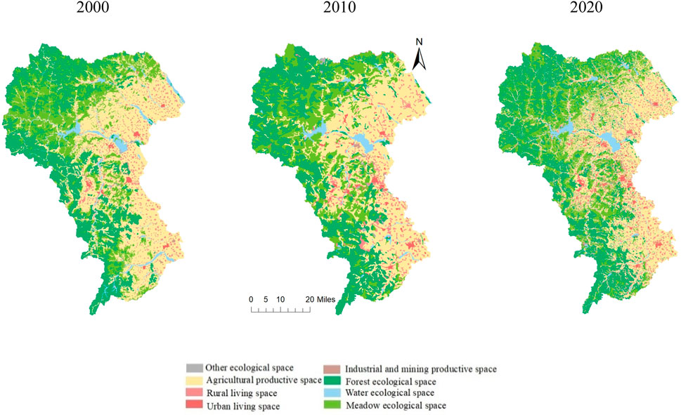
Figure 2. PLES distribution of the TMS during 2000-2020.

3.2 Transition of PLES

To understand the transition of PLES, we calculated the transition structure and transition rates using Eq. 1, and the results are as follows:

From Table 4 we can see that from the perspective of the transfer-in, agricultural productive space was mainly transferred from meadow ecological space, and industrial and mining productive space was mainly transferred from rural productive land. Forest ecological space was mainly transferred from rural productive space and meadow ecological space, water ecological land was mainly transferred from agricultural productive space, and other ecological space was mainly transferred from forest ecological space and meadow ecological space. Urban living space was mainly transferred from agricultural productive space and rural living space, and rural living space was mainly transferred from agricultural productive space.

Table 4

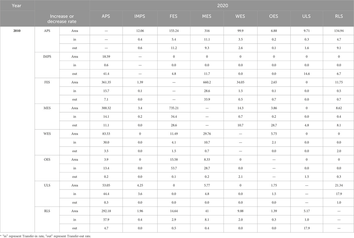
Table 4. Transition matrix and transition rates of PLES during 2000–2020 Unit: km², %.

From the perspective of the transfer-out, agricultural productive space was mainly converted to forest ecological space, meadow ecological space, and rural living space, and industrial and mining productive space was converted to agricultural productive space and urban living space. Forest ecological space was converted to meadow ecological space, and meadow ecological space was converted to forest ecological space and agricultural ecological space; water ecological space was converted to agricultural productive space and forest ecological space, and other ecological space was converted to agricultural productive space and water ecological space. Finally, urban living space was converted to agricultural productive space, and rural living space was converted to agricultural productive space.

With the rapid urbanization of Shijiazhuang City, huge amounts of agricultural productive space and ecological space was occupied by urban living space. With the implementation of a series of ecological engineering projects such as forest rehabilitation from slope agriculture, the cultivated land with serious soil erosion and obvious ecological vulnerability has gradually transformed into ecological space, further restoring the latter.

3.3 Carbon emission effects of PLES

3.3.1 Spatial-temporal evolution of carbon emission

As shown in Table 5, from 2000 to 2020, carbon emissions were 130.96 × 10⁴ t, 387.69 × 10⁴ t, and 222.06 × 10⁴ t, respectively, and carbon storage was 20.11 × 10⁴ t, 17.33 × 10^4 t, and 21.55 × 10⁴ t, respectively. The study area has been in a state of carbon deficit. From the perspective of the changing trend, carbon emissions first rapidly increased by 256.73 × 10⁴ t from 2000 to 2010 and then slowly decreased by 165.63 × 10⁴ t from 2010 to 2020. Carbon storage first decreased by 2.78 × 10⁴ t from 2000 to 2010 and then increased by 4.21 × 10⁴ t from 2010 to 2020. The carbon deficit first increased by 255.84 × 10⁴ t from 2000 to 2010 and then decreased by 165.20 × 10⁴ t from 2010 to 2020.

Table 5

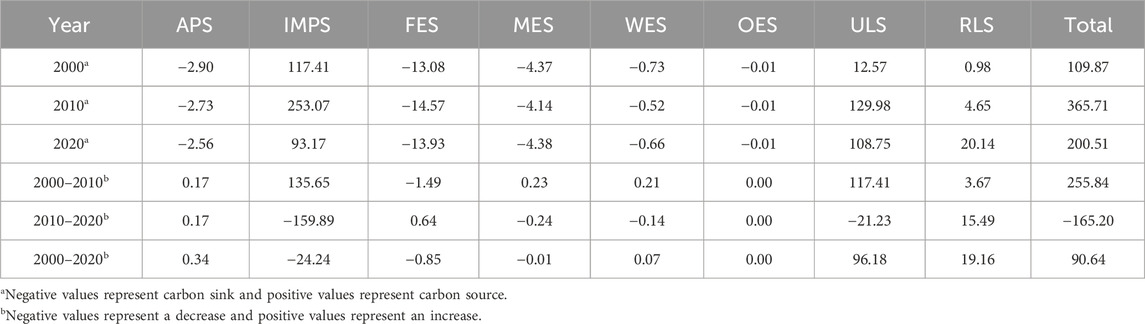
Table 5. Carbon emission structure and changes in PLES. Unit: 10⁴ t.

From the perspective of PLES types, agricultural productive space, as well as forest, meadow, water, and other ecological space were carbon sinks, and industrial and mining productive space, urban living space, and rural living space were carbon sources. From 2000 to 2020, the carbon storage of agricultural productive space has been decreasing, with a total reduction of 0.34 × 10⁴ t. The carbon storage of ecological space first increased by 1.06 × 10⁴ t from 2000 to 2010 and then decreased by 0.26 × 10⁴ t from 2000 to 2020, with a total increase of 0.80 × 10⁴ t. The carbon emissions of industrial and mining space first increased by 135.65 × 10⁴ t from 2000 to 2010 and then decreased by 159.89 × 10⁴ t from 2010 to 2020, with a total reduction of 24.24 × 10⁴ t. The carbon emissions of urban living space first increased by 117.41 × 10⁴ t from 2000 to 2010 and then decreased by 21.23 × 10⁴ t from 2010 to 2020, with a total increase of 96.18 × 10⁴ t. The emissions of rural residential land increased gradually, with a total increase of 19.16 × 10⁴ t. Thus, the carbon emissions have shifted from “high pollution, high emissions” to “low pollution, low emissions.” With the implementation of a series of energy conservation policies, coal consumption has dropped significantly and has been replaced by clean energy such as electricity and natural gas, thereby leading to a obviously decrease in carbon emissions.

The data of PLES and carbon density were input into the ArcGIS 10.8 to obtain the carbon emissions pattern (Figure 3). Carbon emissions were divided into high, medium-high, medium, low-medium, and low levels following the equal-interval method by the means of Nature break Point. As shown in Figure 3, low and low-medium levels of carbon emissions belonging to carbon surplus areas were distributed in agricultural productive space and ecological space, mainly in Xingtang, Lingshou, Pingshan, Jingxin, and Zanhuang County. The medium, medium-high, and high levels belonging to carbon emission areas were distributed in industrial and mining productive space, urban living space, and rural living space, mainly in Luquan District, Jingxing Mining District, Yuanshi County. From the perspective of spatial pattern changes, from 2000 to 2010, the low and low-medium levels decreased significantly, whereas the medium level increased obviously. From 2010 to 2020, the low and low-medium levels were further reduced, and the high-level areas increased.

Figure 3

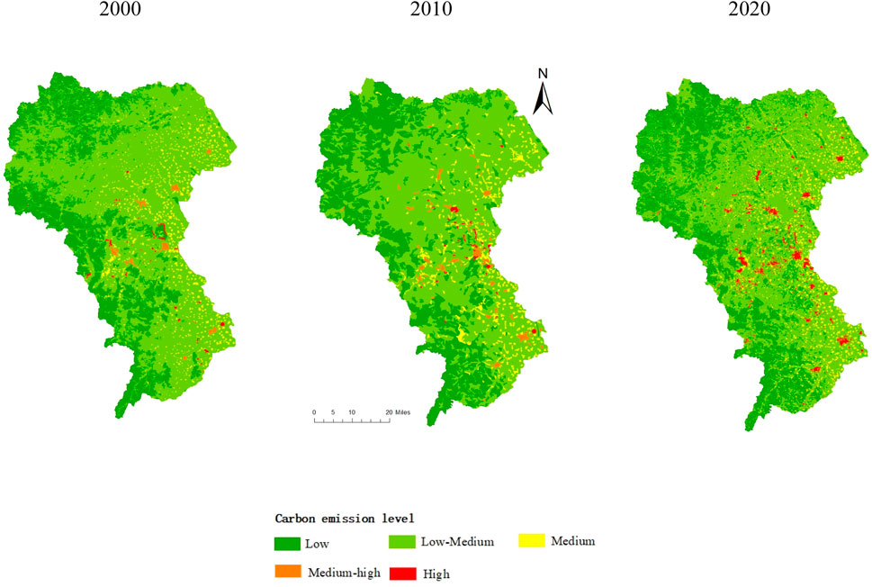
Figure 3. Carbon emission pattern of PLES.

3.3.2 Carbon-emissions contribution rate of PLES

The carbon-emissions contribution rate of PLES was calculated based on Formula 2 (Table 6).

Table 6

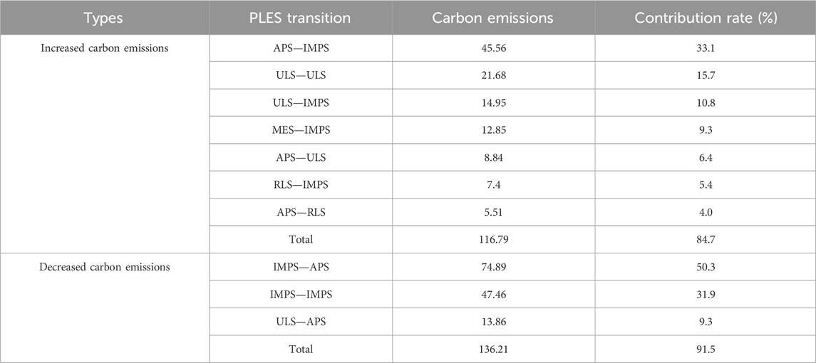
Table 6. Carbon-emissions contribution rate of main PLES transition types Unit: 10⁴ t, %.

The main transition types of carbon emissions were in agricultural productive space, industrial and mining productive space, urban living space, and rural living space. In the transition types caused the carbon emissions increasing, there are two transition directions. One is from carbon sink to carbon source, such as agricultural production space to industrial and mining productive space, urban living space and rural living space, and meadow ecological space to industrial and mining productive space, accounting for 52.8% of the increase in total carbon emissions. The second is from low-to high-density carbon emissions, such as urban living space to industrial and mining productive space, rural living space to urban living space, and urban living space to urban living space, accounting for 31.9% of the increase in total carbon emissions. In the main transition types caused the carbon emissions reduction, the contribution rate of industrial and mining productive space to agricultural productive space was the highest, followed by industrial and mining productive space to itself, and the third is urban living space to agricultural living space. All three account for 91.5% of the total reduction in carbon emissions.

3.3.3 Marginal change in carbon emissions

The marginal change in carbon emissions can reflect the influence of areas on carbon emissions or sink. The marginal carbon emissions of industrial and mining productive space were the highest at 54231.40 t, followed by urban living space at 13493.02 t; those of rural living space were the lowest at 1010.74 t, indicating that the three PLES types were the main carbon emission sources. The marginal carbon sink of forest ecological space was the highest at 60.36 t, followed by water ecological space and water ecological space at 20.52 t and 23.80 t, respectively, whereas those of agricultural productive space and other ecological space were the lowest at 9.002 t and 5.00 t, indicating that the three PLES types were the main carbon sink sources.

3.4 Influencing factors of carbon emissions

3.4.1 Parameter estimation results of panel data model

Based on panel data from 2000 to 2020, this paper used the improved STIRPAT model to analyze the influencing factors using Stata12.0 software. The results were shown in Table 7.

Table 7

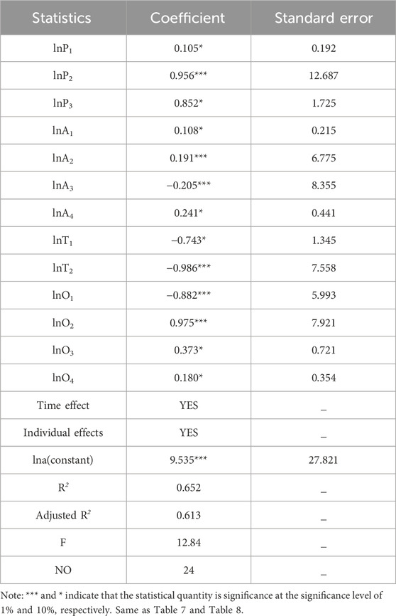
Table 7. Estimated results of fixed effect model.

It can be seen from Table 7, the coefficient of Total population, Population density, Per capita GDP, Foreign direct investment, Per capita energy consumption, Number of industrial enterprises above scale, Per capita disposable income did not pass the t-test, which showed that these indicators did not conform to the Kuznets hypothesis. All the other coefficients passed the t-test under the given condition. The baseline regression equation was:

$\ln C_{it}=9.535+0.956\ln P_2+0.191\ln A_2-0.205\ln A_3-0.986\ln T_2-0.882\ln O_1+0.975\ln O_2(7)$

3.4.2 Analysis of influencing factors

The improved STIRPAT model obtained from the results is shown in Eq. 7. From the fitting results of the model, the order of the effects of the influencing factors was as follows: O₂>P₂>A₂>A₃>O₁>T₂. Among these, the proportion of construction (O₂), land urbanization rate (P₂), and proportion of secondary industry (A₂) were positively correlated with total carbon emissions, while the proportion of tertiary industry (A₃), forest coverage rate (O₁), and per capita energy consumption (T₂) were negatively correlated.

The proportion of construction land (O₂) was the strongest factor for the increase of carbon emissions in the TMS, and the elasticity coefficient was found to be 0.975%, indicating that for every 1% increase in the proportion of construction land, the total carbon emissions will increase by 0.975%. This indicates that the transition of the PLES has a direct impact on carbon emissions. For every 1% increase in urbanization rate (P₂), the proportion of secondary industries (A₂), total carbon emissions will increase by 0.956% and 0.191%, respectively. The study area is located in the poverty belt of the Taihang Mountains, and its economic development had low and late starting points. By accelerating industrialization, the economic level has improved, resulting in excessive energy consumption and high carbon emissions.

Per capita energy consumption (T₂) is the strongest factor in regard to the decrease in carbon emissions, and the elasticity coefficient is −0.986%, indicating that for every 1% increase in per capita energy consumption, the total carbon emissions will decrease by 0.986%. Therefore, improvements in technology can promote improvements in energy-use efficiency, which is an effective way to reduce total carbon emissions.

The influence coefficient of forest coverage rate (O₁), and Per capita energy consumption (A₃) are −0.882% and −0.205%, respectively, and each increase of 1% will decrease the total carbon emissions by 0.882% and 0.205%, respectively. From 2000 to 2020, the forest coverage rate in the TMS increased from 52.16% to 53.9%, which caused the carbon sink value to increase and the net carbon emissions decreased. It can be seen that the transformation of PLES is an important reason for the decrease of carbon emissions. The tertiary industry in the study area has developed rapidly, from 29.75% in 2000 to 52.62% in 2020. Tertiary industries such as tourism and social services have achieved rapid development. It has low carbon emission intensities, which cause a decrease in carbon emissions.

3.4.3 Robustness test

To ensure the reliability of the research results, we conducted a robustness test on the following aspects:

3.4.3.1 Increasing the control variables

To eliminate the influence of the unobservable factors, this study increased the indicator of the proportion of local financial expenditures to GDP and we then conducted a regression analysis once again. In China, the government’s macro-control policies can directly affect industrial structure, energy conservation, and emission reduction technology, thus indirectly affecting carbon emissions. With reference to the relevant literature (Zeng et al., 2019), this study selected an indicator of the proportion of local financial expenditure to GDP as the proxy variable for government macro control. The test results indicate that increasing the indicator is consistent with the baseline regression results, which proves the reliability of the regression results (Table 8).

Table 8

Table 8. Robustness test: increasing control variables.

3.4.3.2 Replace the explained variable

The explanatory variables used in the baseline regression were based on carbon emissions from land-use changes. This study used the total carbon emissions of each county obtained from the Statistical Yearbook as explanatory variables. The test results indicated whether the explained variable was replaced, which was consistent with the baseline regression results, thus proving the reliability of the regression results (Table 9).

Table 9

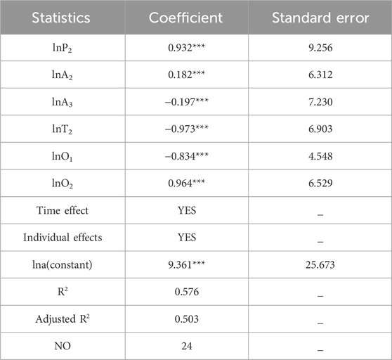
Table 9. Robustness test: replacing the explained variable.

4 Conclusion and discussion

4.1 Discussion

4.1.1 Comparisons between this paper and previous studies

In terms of the transition of the PLES, the PLES in the TMS experienced the process of first decreasing and then increasing ecological space and continuing to increase the living space, which is consistent with the ecological space changes in the mountainous areas of China (Wang and Liu, 2023) and the trends of forest change in Asia (Hansen, 2013). Driven by rapid industrialization and urbanization, the labor force in the mountainous areas has been transferred to cities and towns, leading to natural vegetation restoration and expansion of forestland.

In terms of the carbon emission effects, ecological space is the main source of carbon sinks. The changes seen in the forestland and grassland directly affect the amount of carbon sinks, which is consistent with relevant international research conclusions (Jandl et al., 2007). In recent years, China has vigorously implemented afforestation and strengthened forest management; therefore, the area of ecological space in the TMS has increased, and the carbon sink capacity has improved. The expansion of industrial and mining production and urban living spaces were the main reasons for the increase in carbon emissions, which is consistent with the relevant international research (Grimm et al., 2008; Beesley, 2012; Burgin et al., 2016). However, the difference is that carbon emissions in the study area first increased and then decreased, reflecting it has gone through the process of polluting first and then remediation in the TMS. And it also reflected the conflict in the PLES experienced a process of conflict intensification leading to gradual coordination.

In terms of the factors influencing carbon emissions, urbanization, economic growth, and energy consumption are the main reasons found for the increase in carbon emissions, which is consistent with the research conclusions of developing countries, such as Pakistan and Africa (Aftab et al., 2021; Namahoro et al., 2021). This reflects the enormous pressure on developing countries to reduce carbon emissions. Energy intensity and increased forest area are important reasons for the reduction in carbon emissions, which is consistent with the conclusions of other countries (Ang, 1999; Henriques and Borowiecki, 2017). However, this study argues that the PLES transition, especially the transition between the ecological space and production space, is another important reason for carbon emissions.

4.1.2 Limitations and prospect of this study

Owing to limited data access, this study takes the Taihang Mountain area, located west of Shijiazhuang, as an example to study the transition of the PLES and carbon emissions in the Taihang Mountain area in China, which may not be sufficiently comprehensive.

Due to the complex topography of the TMS, land-use patterns are affected by altitude, slope, aspect, soil erosion, and other factors that may influence carbon emissions. Future studies should consider these factors in relation to carbon emissions.

4.2 Conclusion

In this study, the spatial-temporal evolution characteristics of the PLES transition was explored in the TMS from 2000 to 2020 based on the land-use transfer matrix. Secondly, the carbon effects of the PLES transition were described through the indicators of “Contribution rate” and “Marginal carbon emissions”. Finally, the influencing factors were analyzed by the Improved STIRPAT Model. It can provide a theoretical basis for the optimization of territorial space in the mountainous areas of China. The main conclusions are as follows:

(1) The TMS is mainly composed of ecological space and production space. During the study period, the ecological space and living space increased by 123.80 km² and 260.86 km², respectively, while the production space decreased by 384.66 km². The TMS has been in a state of carbon deficit, and it has experienced a process of increasing first and then decreasing. Carbon storage of ecological space increased by 0.80 × 10⁴t, while that of agricultural productive space decreased by 0.34 × 10⁴t. Carbon emissions of industrial and mining productive space decreased by 24.24 × 10⁴t, while that of living space increased by115.30 × 10⁴t.

(2) The transition between agricultural productive space and industrial and mining productive space was the main transition types caused the increase or decrease of carbon emissions. The marginal carbon emission of industrial and mining productive space was the largest, and the marginal carbon sink of forest ecological space was the largest.

(3) Proportion of construction land was the strongest factor leading to the increase of carbon emissions, with the elasticity coefficient of 0.975%, followed by the factors of urbanization rate and proportion of secondary industry. Per capita energy consumption is the strongest factor leading to the decrease of carbon emissions, with the elasticity coefficient is −0.986%, followed by the factors of forest coverage and proportion of tertiary industry.

4.3 Policy recommendations

Based on the aforementioned analysis, we can formulate different policies according to different territorial space control objectives and gradually coordinate the PLES.

(1) For ecological space, the core is to enhance the carbon sequestration capacity. The carbon storage of forest and meadow ecological space in the TMS is much larger than that of other ecological spaces, so the scale of forestland and grassland can be continuously increased. The vacating space should preferentially restore to forest and meadow ecological space. The carbon sequestration capacity can also be improved by planting local tree species and optimizing the proportion of mixed species.

(2) For agricultural productive space, because it has a certain carbon sequestration capacity, so we should actively develop green agriculture, reduce the application of pesticides and fertilizers, and implement straw returning. Combining with the terrain and climate resources in the study area, develop unique mountain green agriculture. For industrial and mining productive space, reduce pollution energy and increase clean energy to reduce carbon emissions, and establish industrial parks to optimize the layout of industrial production space.

(3) For urban living space, delineate the urban boundary to control the urban expansion. Reasonable arrange the park green space in the urban area to enhance the carbon sequestration capacity. For rural living space, guide moderately intensive arrangement of rural living spaces through village relocation and mergers, and construct modern new rural living space. Increase the area of green land in the village to enhance the carbon sequestration capacity.

Data availability statement

The raw data supporting the conclusion of this article will be made available by the authors, without undue reservation.

Author contributions

JC: Writing–original draft, Writing–review and editing. YZ: Methodology, Writing–review and editing. HD: Data curation, Software, Writing–review and editing. TZ: Supervision, Writing–review and editing.

Funding

The author(s) declare financial support was received for the research, authorship, and/or publication of this article. This research was funded by the Humanities and Social Science Research Project of Hebei Education Department, grant number SQ2023040.

Conflict of interest

The authors declare that the research was conducted in the absence of any commercial or financial relationships that could be construed as a potential conflict of interest.

Publisher’s note

All claims expressed in this article are solely those of the authors and do not necessarily represent those of their affiliated organizations, or those of the publisher, the editors and the reviewers. Any product that may be evaluated in this article, or claim that may be made by its manufacturer, is not guaranteed or endorsed by the publisher.

References

Aftab, S., Ahmed, A., Chandio, A. A., Korankye, B. A., and Fang, W. (2021). Modeling the nexus between carbon emissions, energy consumption, and economic progress in Pakistan: evidence from cointegration and causality analysis. Energy Rep. 7, 4642–4658. doi:10.1016/j.egyr.2021.07.020

CrossRef Full Text | Google Scholar

Ang, B. W. (1999). Is the energy intensity a less useful indicator than the carbon factor in the study of climate change. Energy Policy 27, 943–946. doi:10.1016/S0301-4215(99)00084-1

CrossRef Full Text | Google Scholar

Ang, B. W., Zhang, F. Q., and Choi, K. H. (1998). Factorizing changes in energy and environmental indicators through decomposition. Energy 23 (6), 489–495. doi:10.1016/S0360-5442(98)00016-4

CrossRef Full Text | Google Scholar

Arrow, K., Bolin, B., Costanza, R., Dasgupta, P., Folke, C., Holling, C., et al. (1995). Economic growth, carrying capacity, and the environment. Science 268, 91–95. doi:10.1016/0921-8009(95)00059-3

PubMed Abstract | CrossRef Full Text | Google Scholar

Arshed, N., Munir, M., and Iqbal, M. (2021). Sustainability assessment using STIRPAT approach to environmental quality: an extended panel data analysis. Environ. Sci. Pollut. Res. 28, 18163–18175. doi:10.1007/s11356-020-12044-9

PubMed Abstract | CrossRef Full Text | Google Scholar

Bai, R., Shi, Y., and Pan, Y. (2022). Land-use classifying and identification of the Production-Living-Ecological Space of island villages-A case study of islands in the western sea area of Guangdong Province. Land 11, 705. doi:10.3390/land11050705

CrossRef Full Text | Google Scholar

Balthazar, V., Vanacker, V., Molina, A., and Lambin, E. F. (2015). Impacts of forest cover change on ecosystem services in high Andean mountains. Ecol. Indic. 48, 63–75. doi:10.1016/j.ecolind.2014.07.043

CrossRef Full Text | Google Scholar

Barnett, T. P., Adam, J. C., and Lettenmaier, D. P. (2005). Potential impacts of a warming climate on water availability in snow-dominated regions. Nature 438, 303–309. doi:10.1038/nature04141

PubMed Abstract | CrossRef Full Text | Google Scholar

Beesley, L. (2012). Carbon storage and fluxes in existing and newly created urban soils. J. Environ. Manage. 104, 158–165. doi:10.1016/j.jenvman.2012.03.024

PubMed Abstract | CrossRef Full Text | Google Scholar

Burgin, S., Franklin, M. J. M., and Hull, L. (2016). Wetland loss in the transition to urbanisation: a case study from Western Sydney, Australia. Wetlands 36, 985–994. doi:10.1007/s13157-016-0813-0

CrossRef Full Text | Google Scholar

Chen, L., Zhou, Sh. L., Zhou, B. B., Zhao, K., Wu, X., and Xian, Y. (2015). Characteristics and driving forces of regional land use transition based on the leading function classification: a case study of Jiangsu Province. Econ. Geogr. 35, 155–162. doi:10.15957/j.cnki.jjdl.2015.02.022

CrossRef Full Text | Google Scholar

Chen, X. L. (2003). Research on carbon sequestration functions of main forest types in northern China. Doctor. Beijing: Beijing Forestry University.

Google Scholar

Chen, Z., Liu, Y., and Tu, S. (2022). Comprehensive eco-environmental effects caused by land use transition from the perspective of Production–Living–Ecological Spaces in a typical region: a case study of the Guangxi Zhuang Autonomous Region, China. Land 11, 2160. doi:10.3390/land11122160

CrossRef Full Text | Google Scholar

Chontanawat, J. (2018). Decomposition analysis of CO₂ emission in ASEAN: an extended IPAT model. Energy Procedia 153, 186–190. doi:10.1016/j.egypro.2018.10.057

CrossRef Full Text | Google Scholar

Cui, X., Xu, N., Chen, W., Wang, G., Liang, J., Pan, S., et al. (2022). Spatio-temporal variation and influencing factors of the coupling coordination degree of production-living-ecological space in China. Int. Environ. Res. Public Health 19, 10370. doi:10.3390/ijerph191610370

CrossRef Full Text | Google Scholar

Data Center for Resources and Environmental Sciences, Chinese Academy of Sciences (RESDC) (2018). China land use/land cover remote sensing monitoring data classification system. Beijing, China: RESDC.

Google Scholar

Deslatte, A., Szmigiel-Rawska, K., Tavares, A. F., Ślawska, J., Karsznia, I., and Łukomska, J. (2022). Land use institutions and social-ecological systems: a spatial analysis of local landscape changes in Poland. Land Use Policy 114, 105937. doi:10.1016/j.landusepol.2021.105937

CrossRef Full Text | Google Scholar

de Sousa-Neto, E. R., Gomes, L., Nascimento, N., Pacheco, F., and Ometto, J. P. (2018). Land use and land cover transition in Brazil and their effects on greenhouse gas emissions. Soil Manag. Clim. Change, 309–321. doi:10.1016/B978-0-12-812128-3.00020-3

CrossRef Full Text | Google Scholar

Drummond, M. A., Griffith, G. E., Auch, R. F., Stier, M. P., Taylor, J. L., Hester, D. J., et al. (2017). Understanding recurrent land use processes and long-term transitions in the dynamic south-central United States, c. 1800 to 2006. Land Use Policy 68, 345–354. doi:10.1016/j.landusepol.2017.07.061

CrossRef Full Text | Google Scholar

Duan, Y., Wang, H., Huang, A., Xu, Y., Lu, L., and Ji, Z. (2021). Identification and spatial-temporal evolution of rural "production-living-ecological" space from the perspective of villagers' behavior-A case study of Ertai Town, Zhangjiakou City. Land Use Policy 106, 105457. doi:10.1016/j.landusepol.2021.105457

CrossRef Full Text | Google Scholar

Fahey, T. J., Woodbury, P. B., Battles, J. J., Goodale, C. L., Hamburg, S. P., Ollinger, S. V., et al. (2010). Forest carbon storage: ecology, management, and policy. Front. Ecol. Environ. 8, 245–252. doi:10.1890/080169

CrossRef Full Text | Google Scholar

Gao, H., Fu, T. G., Liu, J. T., Liang, H., and Han, L. (2018). Ecosystem services management based on differentiation and regionalization along vertical gradient in Taihang Mountain, China. Sustainability 10 (4), 986–1000. doi:10.3390/su10040986

CrossRef Full Text | Google Scholar

Goldewijk, K. K. (2001). Estimating global land use change over the past 300 years: the HYDE Database. Glob. Biogeochem. Cycles 15 (2), 417–433. doi:10.1029/1999GB001232

CrossRef Full Text | Google Scholar

Grimm, N. B., Faeth, S. H., Golubiewski, N. E., Redman, C. L., Wu, J. G., Bai, X. M., et al. (2008). Global change and the ecology of cities. Science 319, 756–760. doi:10.1126/science.1150195

PubMed Abstract | CrossRef Full Text | Google Scholar

Hansen, M. C., Potapov, P. V., Moore, R., Hancher, M., Turubanova, S. A., Tyukavina, A., et al. (2013). High-resolution global maps of 21st-century forest cover change. Science 342, 850–853. doi:10.1126/science.1244693

PubMed Abstract | CrossRef Full Text | Google Scholar

Henriques, T. S., and Borowiecki, K. J. (2017). The drivers of long-run CO₂ emissions in Europe, North America and Japan since 1800. Energy Policy 101, 537–549. doi:10.1016/j.enpol.2016.11.005

CrossRef Full Text | Google Scholar

Hidemichi, F., Kazuyuki, I., Andrew, C., Kagawa, S., and Managi, S. (2018). An analysis of urban environmental Kuznets curve of CO₂ emissions: empirical analysis of 276 global metropolitan areas. Appl. Energy 228, 1561–1568. doi:10.1016/j.apenergy.2018.06.158

CrossRef Full Text | Google Scholar

Houghton, R. A. (2018). Interactions between land-use change and climate-carbon cycle feedbacks. Curr. Clim. Change Rep. 4, 115–127. doi:10.1007/S40641-018-0099-9

CrossRef Full Text | Google Scholar

Houghton, R. A., and Hackler, J. L. (1999). Emissions of carbon from forestry and land-use change in tropical Asia. Glob. Change Biol. 5, 481–492. doi:10.1046/j.1365-2486.1999.00244.x

CrossRef Full Text | Google Scholar

Houghton, R. A., House, J. I., Pongratz, J., van der Werf, G. R., DeFries, R. S., Hansen, M. C., et al. (2012). Carbon emissions from land use and land-cover change. Biogeosciences 9 (12), 5125–5142. doi:10.5194/bg-9-5125-2012

CrossRef Full Text | Google Scholar

Hu, G. X., Lei, G. P., and Zhou, H. (2015). Effects of different land use patterns on carbon emission in heilongjiang province. Res. Soil Water Conservation 22 (6), 287–292. doi:10.13869/j.cnki.rswc.2015.06.040

CrossRef Full Text | Google Scholar

Jandl, R., Lindner, M., Vesterdal, L., Bauwens, B., Baritz, R., Hagedorn, F., et al. (2007). How strongly can forest management influence soil carbon sequestration? Geoderma 137, 253–268. doi:10.1016/j.geoderma.2006.09.003

CrossRef Full Text | Google Scholar

Jiang, X. T., Zhai, S. Y., Liu, H., Chen, J., Zhu, Y., and Wang, Z. (2022). Multi-scenario simulation of production-living-ecological space and ecological effects based on shared socioeconomic pathways in Zhengzhou, China. Ecol. Indic. 137, 108750. doi:10.1016/j.ecolind.2022.108750

CrossRef Full Text | Google Scholar

Kong, D. Y., Chen, H. G., and Wu, K. S. (2021). The evolution of "Production-Living-Ecological" space, eco-environmental effects and its influencing factors in China. J. Nat. Resour. 36, 1116–1135. doi:10.31497/zrzyxb.20210503

CrossRef Full Text | Google Scholar

Lambin, E. F., and Meyfroidt, P. (2011). Global land use change, economic globalization, and the looming land scarcity. Proceedings of the National Academy of Sciences of the United States of America 108 (9), 3465–3472. doi:10.1073/pnas.1100480108

PubMed Abstract | CrossRef Full Text | Google Scholar

Li, X. S., Li, Zh.X., and Xie, X. T. (2023). Analysis of the interaction mechanism of urbanization, carbon emissions, and production-living-ecological space in Henan Province of China. Trans. CSAE 39(11), 256–265.

Google Scholar

Li, Y. H. (2020). Measure of the impact of fiscal decentralization on carbon emissions based on the STIRPAT model. Stat. Decis. 19, 136–140. doi:10.13546/j.cnki.tjyjc.2020.18.031

CrossRef Full Text | Google Scholar

Liao, G., He, P., Gao, X., Lin, Z., Huang, C., Zhou, W., et al. (2022). Land use optimization of rural production-living-ecological space at different scales based on the BP-ANN and CLUE-S models. Ecol. Indic. 137, 108710-. doi:10.1016/j.ecolind.2022.108710

CrossRef Full Text | Google Scholar

Liu, T. H., Ji, Z. X., Duan, Y. M., and Xu, Y. Q. (2023). Spatial pattern evolution and carbon effect of production-living-ecological space in Zhangjiakou city under carbon peak and carbon neutrality goals. Acta Sci. Nat. Univ. Pekin. 59 (3), 513–522. doi:10.13209/j.0479-8023.2023.025

CrossRef Full Text | Google Scholar

Luan, W. L., Song, Z. F., and Li, S. M. (2011). Changes of soil organic carbon content in Hebei Plain. Acta Geogr. Sin. 85, 1528–1535.

Google Scholar

Namahoro, J. P., Wu, Q., Zhou, N., and Xue, S. (2021). Impact of energy intensity, renewable energy, and economic growth on CO₂ emissions: evidence from Africa across regions and income levels. Renew. Sustain. Energy Rev. 2021, 111233. doi:10.1016/j.rser.2021.111233

CrossRef Full Text | Google Scholar

Newbold, T., Hudson, L. N., Hill, S. L. L., Contu, S., Lysenko, I., Senior, R. A., et al. (2015). Global effects of land use on local terrestrial biodiversity. Nature 520 (7545), 45–50. doi:10.1038/nature14324

PubMed Abstract | CrossRef Full Text | Google Scholar

Nosheen, M., Abbasi, M. A., and Iqbal, J. (2020). Analyzing extended STIRPAT model of urbanization and CO₂ emissions in Asian countries. Environ. Sci. Pollut. Res. 27, 45911–45924. doi:10.1007/s11356-020-10276-3

PubMed Abstract | CrossRef Full Text | Google Scholar

Ojoyi, M. M., Mutanga, O., Odindi, J., Kahinda, J. M. M., and Abdel-Rahman, E. M. (2017). Implications of land use transitions on soil nitrogen in dynamic landscapes in Tanzania. Land Use Policy 64, 95–100. doi:10.1016/j.landusepol.2017.02.023

CrossRef Full Text | Google Scholar

Schimel, D. S. (2010). Terrestrial ecosystems and the carbon cycle. Glob. Change Biol. 1 (1), 77–91. doi:10.1111/j.1365-2486.1995.tb00008.x

CrossRef Full Text | Google Scholar

Shahbaz, M., Loganathan, N., Sbia, R., and Afza, T. (2015). The effect of urbanization, affluence and trade openness on energy consumption: a time series analysis in Malaysia. Renew. Sustain. Energy Rev. 47 (11), 683–693. doi:10.1016/j.rser.2015.03.044

CrossRef Full Text | Google Scholar

Tian, F., Li, M., Han, X., Liu, H., and Mo, B. (2020). A production-living-ecological space model for land-use optimisation: a case study of the core Tumen River region in China. Ecol. Model. 437, 109310. doi:10.1016/j.ecolmodel.2020.109310

CrossRef Full Text | Google Scholar

Vujovi, T., Petkovi, Z., Pavlovi, M., and Jović, S. (2018). Economic growth based in carbon dioxide emission intensity. Phys. A Stat. Mech. its Appl. S0378437118305028 506, 179–185. doi:10.1016/j.physa.2018.04.074

CrossRef Full Text | Google Scholar

Wang, A., Liao, X., Tong, Z., Du, W., Zhang, J., Liu, X., et al. (2022). Spatial-temporal dynamic evaluation of the ecosystem service value from the perspective of “production-living-ecological” spaces: a case study in Dongliao River Basin, China. J. Clean. Prod. 333, 130218. doi:10.1016/j.jclepro.2021.130218

CrossRef Full Text | Google Scholar

Wang, S., and Liu, F. (2023). Spatiotemporal evolution of land use efficiency in southwest Mountain area of China: a case study of yunnan province. Agriculture 13, 1343. doi:10.3390/agriculture13071343

CrossRef Full Text | Google Scholar

Wang, Y., Yang, G., Dong, Y., Cheng, Y., and Shang, P. (2018). The scale, structure and influencing factors of total carbon emissions from households in 30 provinces of China—based on the extended STIRPAT Model. Energies 11, 1125. doi:10.3390/en11051125

CrossRef Full Text | Google Scholar

Weber, A., Fohrer, N., and Mo¨ller, D. (2001). Long-term land use changes in a mesoscale watershed due to socio-economic factors-effects on landscape structures and functions. Ecol. Model. 140 (1-2), 125–140. doi:10.1016/S0304-3800(01)00261-7

CrossRef Full Text | Google Scholar

Winkler, K., Fuchs, R., Rounsevell, M., and Herold, M. (2021). Global land use changes are four times greater than previously estimated. Nat. Commun. 12, 2501. doi:10.1038/s41467-021-22702-2

PubMed Abstract | CrossRef Full Text | Google Scholar

Woodbury, P. B., Heath, L. S., and Smith, J. E. (2007). Effects of land use change on soil carbon cycling in the conterminous United States from 1900 to 2050. Glob. Biogeochem. Cycles 21 (3). doi:10.1029/2007GB002950

CrossRef Full Text | Google Scholar

Yang, Q. K., Duan, X. J., and Wang, L. (2018). Land use transformation based on ecological-production-living spaces and associated eco-environment effects: a case study in the Yangtze River Delta. Sci. Geogr. Sin. 38, 97–106. doi:10.13249/j.cnki.sgs.2018.01.011

CrossRef Full Text | Google Scholar

Yang, Y., Bao, W., and Liu, Y. (2020). Coupling coordination analysis of rural production-living-ecological space in the Beijing-Tianjin-Hebei region. Ecol. Indic. 117 (4), 106512. doi:10.1016/j.ecolind.2020.106512

CrossRef Full Text | Google Scholar

Yang, Y. Y., Bao, W. K., Li, Y. H., Wang, Y., and Chen, Z. (2020). Land use transition and its eco-environmental effects in the Beijing-Tianjin-Hebei urban agglomeration: a production-living-ecological perspective. Land 9, 285. doi:10.3390/land9090285

CrossRef Full Text | Google Scholar

York, R., Rose, E., and Dietz, T. (2003). STIRPAT, IPAT and Impact: analytic tools for unpacking the driving forces of environmental impacts. Ecol. Econ. 46, 351–365. doi:10.1016/S0921-8009(03)00188-5

CrossRef Full Text | Google Scholar

Zeng, L., Lu, H., Liu, Y., Zhou, , and Hu, (2019). Analysis of regional differences and influencing factors on China's carbon emission efficiency in 2005-2015. Energies12 16, 3081. doi:10.3390/en12163081

CrossRef Full Text | Google Scholar

Zhang, B. L., Gao, J. B., Gao, Y., Cai, W. M., and Zhang, F. R. (2018). Land use transition of mountainous rural areas in China. Acta Geogr. Sin. 73, 503–517.

Google Scholar

Zhang, D., Wang, Z., Li, S., and Zhang, H. (2021). Impact of land urbanization on carbon emissions in urban agglomerations of the middle reaches of the yangtze river. Int. J. Environ. Res. Public Health 18, 1403. doi:10.3390/ijerph18041403

PubMed Abstract | CrossRef Full Text | Google Scholar

Zhang, H. Q., Xu, E. Q., and Zhu, H. Y. (2017). Ecological-Living-Productive land classification system in China. J. Resour. Ecol. 8, 121–128. doi:10.5814/j.issn.1674-764x.2017.02.002

CrossRef Full Text | Google Scholar

Zhao, R. Q., Huang, X. J., and Zhong, T. Y. (2010). Research on carbon emission intensity and carbon footprint of different industrial spaces in China. Acta Geogr. Sin. 65, 1048–1057.

Google Scholar

Zhao, T., Cheng, Y., Fan, Y., and Fan, X. (2022). Functional tradeoffs and feature recognition of rural Production-Living-Ecological Spaces. Land 11, 1103. doi:10.3390/land11071103

CrossRef Full Text | Google Scholar

Zheng, Y. W., Liu, X. H., Xiong, M. Q., Li, F. J., Fu, Y. J., Zhang, Z. F., et al. (2022). Spatial-temporal characteristics of ecological-living-productive land and its carbon emissions in Xinjiang from 1990 to 2018. Pratacultural Sci. 39 (12), 2565–2577. doi:10.11829/j.issn.1001-0629.2022-0294

CrossRef Full Text | Google Scholar

Zhou, K. L., Yang, J. N., Yang, T., and Ding, T. (2023). Spatial and temporal evolution characteristics and spillover effects of China’s regional carbon emissions. J. Environ. Manage. 325, 116423. doi:10.1016/j.jenvman.2022.116423

PubMed Abstract | CrossRef Full Text | Google Scholar

Zhu, W. B., Zhang, J. J., Cui, Y. P., et al. (2019). Assessment of territorial ecosystem carbon storage based on land use change scenario: a case study in Qihe River Basin. Acta Geogr. Sin. 74, 446–459.

Google Scholar