 Zhenkun Wang1
 Zhihong An2*
- 1Beijing Feature Map Technology Co., Ltd, Beijing, China
- 2China Aero Geophysical Survey and Remote Sensing Center for Natural Resources, Beijing, China
Multi-time scale assessment of ecological restoration effects based on objective and scientific approaches can provide crucial information for implementing environmental protection policies and ensuring sustainable regional development. This study evaluated the effect of ecological restoration based on a natural evolution as a reference frame, using yearly Landsat time series. Southern Ningxia in China was selected as the study area. The remote sensing ecological index (RSEI) was calculated. The features of natural evolution were derived from the time series of the RSEI in the natural reserve areas (NRAs). LandTrendr was employed to characterize the disturbance–recovery processes. Furthermore, we adopted the dynamic time-warping method for the entire study period, along with the relative variation ratio (during the disturbance–recovery cycle) to capture the long-term and short-term ecological restoration effects, respectively. The following conclusions were drawn: First, a time-series RSEI based on LandTrendr was used to successfully monitor disturbance–recovery processes. Second, the majority of RSEI disturbances (i.e., >60%) occurred between 2000 and 2005. It is characterized by fewer disturbance times and obvious spatial heterogeneity in disturbance duration. Notably, from 2000 to 2022, the RSEI improved. Additionally, approximately 40% of the study area portrayed a strong similarity to the RSEI of the NRAs. We conclude that quantifying the ecological restoration effect at multi-time scales is a practical operational approach for policymakers and environmental protection. Our study presents novel insights for assessing regional ecological quality, by capturing the processes of natural evolution features in NRAs.
1 Introduction
With substantial population growth and the rapid development of the society and global economy, urbanization and industrialization are expanding exponentially, resulting in regional land degradation and environmental change (Tian et al., 2021; Sikder et al., 2022). The cumulative effects of intensified anthropogenic activities have a significant ecological influence on the natural environment, e.g., declining biodiversity, soil erosion, habitat degradation, and a reduction in habitat diversity (Qu et al., 2020; Cao et al., 2022; Shang et al., 2022). Therefore, an accurate assessment of the ecological environmental quality and restoration effects in a natural reserve area (NRA) can provide crucial information for the implementation of effective environment-protection policies in the area (Liang et al., 2019); this information can serve biodiversity conservation (Yang, 2021), regional sustainable development (Lu et al., 2015; Shan et al., 2019), and ecological civilization construction (Dong et al., 2020).
With the development of remote sensing technology, satellite imagery has become an important approach for analyzing ecological environmental quality and the effects of ecological restoration policies and plans. To monitor the ecological conditions in a region, some scholars developed remote sensing-based parameters, such as the ecological environmental status (Wang et al., 2019), scaled drought condition (Rhee et al., 2010), and aggregate drought (Keyantash and Dracup, 2004) indices, using simple weighting methods (e.g., least square method, analytic hierarchy process, and principal component analysis) (Yang et al., 2020; Dai et al., 2023). To ensure a comprehensive quantitative evaluation of the ecological environment quality, previous studies determined the weights of the abovementioned integrated ecological indices; however, these integrated ecological indices yielded divergent assessment results (Liu et al., 2019; Xiong et al., 2021). The integrated requirements of ecosystems can only be fulfilled by conducting detailed studies that incorporate ecosystem status assessments (Qiao et al., 2021; Zhou et al., 2021). The remote sensing ecological index (RSEI) was established by integrating four indicators (i.e., humidity, greenness, temperature, and aridity) into principal component analysis (Xu, 2013); it can be calculated based on remotely sensed bands from identical satellite sensors, without weight determination (Yi et al., 2023). Notably, a dynamic change in the RSEI is generally correlated to environmental pressures caused by anthropogenic activities (e.g., urbanization and industrialization) (Boori et al., 2021), ecosystem change (e.g., changes in vegetation cover) (Yang et al., 2022), and climatic fluctuations (e.g., changes in temperature and humidity) (Zheng et al., 2022); thus, the RESI can be employed for improving the continuous dynamic assessment of the ecological restoration effects in a region (Zhang et al., 2022; Xiao et al., 2023).
Previous studies have indicated that the variations in ecological environmental quality can be induced by a series of ecological programs, including artificial and natural restoration programs. To evaluate the effectiveness of ecological restoration projects, some studies quantitatively analyzed the time-series trends of individual ecological factors (e.g., through RSEI) or vegetation indices [e.g., normalized difference vegetation index (NDVI) and enhanced vegetation index (EVI)] (Shen et al., 2018; Zhang et al., 2018; Xu et al., 2020). Some studies have used change detection algorithms and models to evaluate the ecological restoration effects in different regions and identify the abrupt points in the time series of comprehensive ecological indices, e.g., continuous change detection and classification, continuous monitoring of land disturbance, Landsat-based detection of the trends in disturbance and recovery, breaks for additive seasonal and trend (BFAST), and vegetation change tracker (Huang et al., 2010; Verbesselt et al., 2010; Zhu and Woodcock, 2014; Zhang et al., 2018; Zhu et al., 2020). For example, short-term abrupt changes (disturbance time and recovery rate) in the gross primary productivity have been analyzed to describe and quantify vegetation health (Li et al., 2023). Significant progress has been made in the assessment of ecological restoration effects. However, the existing literature lacks comprehensive assessments that focus on the short-term changes and long-term trends in the ecological environment, resulting in uncertainties in the current knowledge of ecological restoration processes (Li et al., 2023; Wei et al., 2023). Further, it is difficult to provide an objective assessment of the effects of ecological restoration, owing to the non-consideration of the natural conditions (Li et al., 2017) of a region and the environmental change response at the global scale (Guo et al., 2022).
Priority should be given to selecting a reference framework and developing an effective method for carrying out a comprehensive and objective assessment of the ecological restoration effects in a region. An ideal ecological reference framework and a time-series-based analysis of the ecological environment quality indicators can provide a comprehensive and objective analysis of the effects of restoration in an area (He et al., 2020). As an ideal ecological reference for a definite time series, a previous study carried out an ecological restoration effect assessment to determine the probabilities of the influences of similar ecological indices (e.g., RSEI) between a study region and a natural reserve area (e.g., national parks and national forest parks) (Wang et al., 2022). A majority of existing studies adopt the dynamic time-warping (DTW) method; based on the time-series decomposition and shifting effects, the optimal path among the two time-series (Keogh and Pazzani, 2001) is identified, which is then used to calculate the optimal distance (i.e., similarity weight) between two long time-series images (Tang et al., 2020).
In this study, we used an NRA as an ideal ecological reference area to assess the ecological restoration effect in the study area (southern Ningxia). Furthermore, we developed a framework to analyze the ecological restoration effects in the region using the Landsat data from the perspectives of short- and long-term schemes, based on change-detection algorithms and the DTW model. This study provides a comprehensive and objective analysis of the regional effects of ecological restoration.
2 Study area
We selected the semi-arid and sub-humid loess hilly ecoregion located in southern Ningxia (105°19′–106°57′ E and 35°11′–36°31′ N) as the study area (Figure 1). Encompassing an area of 15,526 km2, this region, which is a part of the northwestern Loess Plateau, is one of Ningxia’s three recognized ecological functional zones, characterized by high ecological vulnerability and sensitivity (Li et al., 2015; Dong et al., 2023; Wei et al., 2023). It covers the Liupan Mountain and Qingshui Valley and is characterized by elevations ranging from 1,305 m to 2,936 m above sea level (asl) (Figure 1C). The average temperature of the region fluctuates between 6.7°C and 8.8°C, while precipitation varies from 458.6 mm to 668.2 mm; the sunshine duration ranges from 2056.9 h to 2,384.4 h annually (Meng et al., 2022). However, the area is significantly impacted by severe drought and extensive anthropogenic activities, e.g., large-scale deforestation and land reclamation, resulting in considerable ecological damage. Since 2000, the Chinese government has implemented a series of ecological restoration policies and actions to address the severe environmental issues in the area (Li et al., 2013; Qiu et al., 2018; Ji et al., 2021). Five NRAs are distributed in the study area (namely, Liupanshan, Nanhuashan, Huoshizhai, Yunwushan, and Zhenhu), covering mountain grassland and meadows, mountain forest scrub meadows, typical grassland ecosystems (in the semi-arid area of the Loess Plateau), and water conservation forests (Yin et al., 2023). The detailed descriptions of the five NRAs are presented in Table 1. The land cover in this region consists of three main types: forest, farmland, and grassland (Figure 1B).
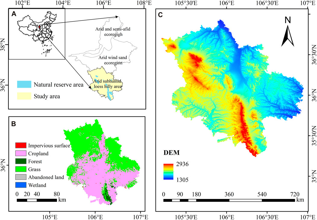
FIGURE 1. (A) Location of the study area in Ningxia, China; (B) distribution of land cover types in the area; and (C) digital elevation model (DEM) of the region.
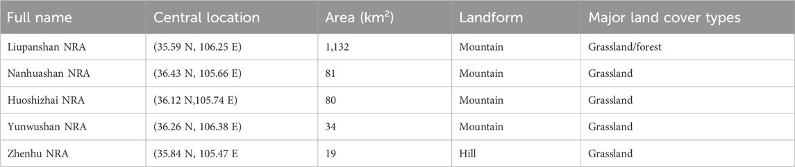
TABLE 1. Detail descriptions of the natural reserve areas (NRAs) considered in this study as reference ecological areas.
3 Materials and methods
The workflow for monitoring the variations in the RSEI and the ecological restoration effects can be summarized as follows (for details, please see Figure 2): 1) RSEI for the study period were calculated (Figure 2A). 2) The variations in the RSEI were analyzed (Figure 2B). 3) To derive the cover of natural vegetation in the region, the multi-order adjacency index was computed (i.e., grass and forest) using a spatiotemporal restoration evolution model (Figure 2C). 4) Finally, the long-term and short-term effects of ecological restoration in the study area were evaluated (Figure 2D).

FIGURE 2. Flowchart portraying the step-by-step methodology employed for evaluating the ecological restoration effects and the variations in the remote sensing ecological index (RSEI): (A) Calculation of remote sensing ecological index; (B) Analysis of RSEI change; (C) Deriving of vegetation restoration spatio-temporal evolution; (D) Evaluating of ecological restoration effect.
3.1 Data preprocessing
In this study, we utilized the surface reflectance data obtained from the Landsat-5, Landsat-7, and Landsat-8 sensors recorded from 2000 to 2022; the data were sourced from the United States Geological Survey (USGS) (Figure 2) and processed using the Google Earth Engine cloud platform (Gorelick et al., 2017). The Landsat images were preprocessed for atmospheric and geometric corrections using the Landsat Ecosystem Disturbance Adaptive Processing System (Masek et al., 2006). To ensure high-quality observations, the pixel band of the CFmask algorithm was utilized to filter clouds, cloud shadows, and snow pixels (Zhu and Woodcock, 2014), thus, retaining the remaining pixels to construct the time-series data for the study area. As this study focused on long-term ecosystem changes, it was essential to integrate the Landsat-5, Landsat-7, and Landsat-8 data, to standardize the vegetation index time series and harmonize the band reflectance values (Zhu et al., 2016). The total number of Landsat images used in this paper with the coverage of cloud less than 20% was displayed in Figure 3. Due to the similarities in their bandwidth and position, the reflectance data measured by the Thematic Mapper (TM) and Enhanced Thematic Mapper Plus (ETM+) sensors were comparable, allowing for their cross-calibration with the Landsat-5 (TM) and Landsat-7 (ETM+) data, as demonstrated in previous studies (Chander et al., 2009).
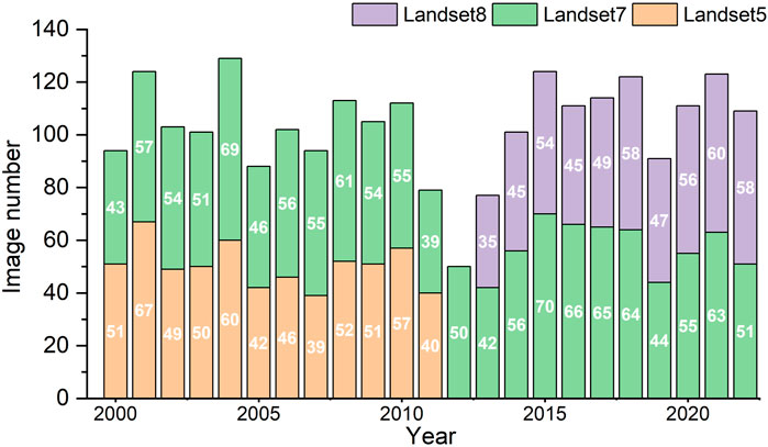
FIGURE 3. Landsat images used in this study.
3.2 Calculation of ecological environmental quality indices
The RSEI, a comprehensive evaluation measure introduced by Xu (2013) to assess the ecosystem quality includes the parameters of greenness, wet, heat, and dryness—four indicators that are intricately connected to human survival (Hu and Xu, 2018; Zheng et al., 2022). The index was calculated using Eq. 1.
In this study, we used the NDVI, soil moisture monitoring index (SMMI), land surface temperature (LST), and normalized difference build-up and soil index (NDBSI) to characterize the abovementioned indicators (Xu, 2013; Xiao et al., 2023). Furthermore, we employed principal component analysis (PCA) for minimizing the errors that result from human intervention and integrate the NDVI, SMMI, LST, and NDBSI. The equations used for calculating the four indices are shown below:
where
SMMI is sensitive to humidity. where swir1 represent the spectral reflectance of short-wave infrared band [1.55–1.75 µm for the TM/ETM + sensors and 1.57–1.65 µm for the Operational Land Imager (OLI)].
The heat index is expressed in terms of surface temperature LST, where
where r, g, and b represent the red, green, and blue bands, respectively. The NDBSI is expressed as the average of
All the calculations were performed using GEE, and normalization was applied to all indices. As the first principal component did not contribute to 85% (based on the results after performing the PCA), we weighted the first two principal components, which yielded a cumulative contribution of >85%.
3.3 Variations in ecological environmental quality
Detecting the disturbances in ecological environmental quality is essential for understanding the effects of anthropogenic activity on the variations in the ecological environmental quality of a region. Landsat-based detection methods (e.g., LandTrendr), used for identifying such disturbance and analyzing recovery trends, are widely used for detecting forest disturbance. Recently, LandTrendr has been widely applied in various fields, e.g., for permafrost thaw monitoring and dynamic mapping of mangroves (de Jong et al., 2021; Runge et al., 2022). The LandTrendr trajectory segmentation method is used to detect changes based on the spectral-temporal segmentation algorithms, for a time-series of moderate-resolution satellite images (primarily Landsat); this process typically comprises of five stages: removing spikes, detecting the potential vertices, fitting the time-series trajectories, optimizing the model, and identifying the best-fitting model (Kennedy et al., 2010). In this study, the LandTrendr algorithm was used to identify the variations in the ecological environmental quality of the study area (Figure 4A); the RSEI time-series trajectories were input into the LandTrendr algorithm on the GEE platform. The control parameter values, including the maximum number of segments, had no effect on the results; therefore, we adopted the default parameters to simplify the workflow.
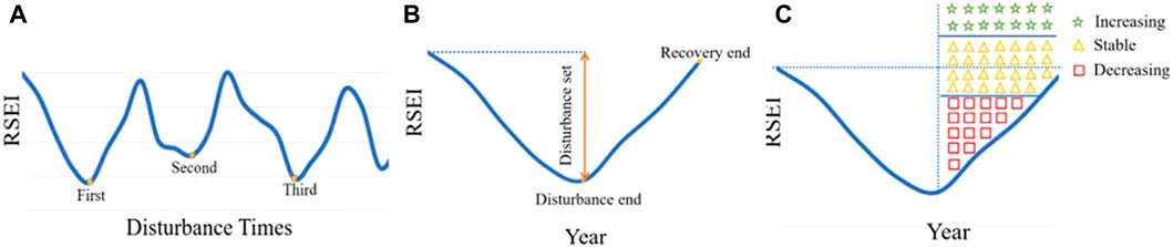
FIGURE 4. Conceptual model portraying the variations in the ecological environmental quality of the study area based on the LandTrendr data: (A) disturbance times; (B) disturbance parameters; (C) trend.
Notably, LandTrendr can capture short-duration events and smooth long-term trends from the spectral trajectories of the changes in the ecological environmental quality, based on the yearly Landsat time-series RSEI. Therefore, metrics such as disturbance, recovery and trend were derived by considering specific events and longer-duration processes. The three kinds of parameters used to analyze the variations in the RSEI were statistically quantified based on the disturbance and recovery parameters and trends (Figure 4).
3.3.1 Disturbance and recovery parameters
The starting and ending points of the segments denote the vertices whose time positions and RSEI values provide the disturbance and recovery information. The disturbance and recovery parameters are presented in Figure 4B. The parameters for disturbance and recovery were derived from the RSEI time series (Table 2). The spatiotemporal distributions of the ecological environmental quality parameters were obtained by setting an optimal threshold for the disturbance magnitude, with a significant difference between the NRAs and study areas. Overall, 1,155 samples from the NRA and 1,133 samples from the study area were selected to determine the ideal threshold for our analysis. We applied the pixels for which the magnitudes were greater than the threshold.

TABLE 2. Definition of disturbance and recovery parameters in this study.
3.3.2 Trend
“Trend” can be denoted as the pattern of oscillations between the disturbance onset and the recovery-end measurements of ecological environmental quality (Figure 4C), portraying decreasing, increasing, or stable trends from the disturbance onset to the recovery end, which can be derived using the Mann–Kendall (MK) non-parametric analysis method (at significance level of α = 0.05) (Czerwinski et al., 2014). Decreasing, increasing, or stable trends are important to assess the ecological environmental quality of a region because they can be indicative of degradation, evolution, or stability, respectively.
3.4 Deriving a spatial evolution model for vegetation restoration
The multistage adjacency index (MAI) can quantitatively analyze the expansion characteristics between the newly added and existing patches, with respect to their spatial relationship, using a multistage buffer zone approach (Liu et al., 2018); notably, this approach was originally used to describe the expansion types for urban landscapes and precisely capture the characteristics of the urban expansion process. The MAI can be calculated using Eq. 9:
where K is the number of buffers for each added patch,
In this work, we considered six growth types for analyzing the vegetation restoration evolution in the study area (using the spatiotemporal model): edge, adjacent, intermediate, separate, and spread expansions and inner filling, in accordance with the approaches employed in previous studies (Liu and Xu, 2021; Liu et al., 2022) (Figure 5). “Inner filling” primarily portrays the specific scenario wherein newly added patches fill the gaps within the pre-existing forest patches, corresponding to the natural recovery process of vegetation. The “edge expansion” growth pattern can be used to plan and develop land use based on the foundation of existing patches. The other four expansions (adjacent, intermediate, separate, and spread) were used to develop and expand specialized industries in the study area, through the large-scale planting of economic trees (e.g., fast-growing timber species). “Separate expansion” and “spread expansion” were used to describe the gradual natural expansion in the study area, portraying the distinct patterns of natural and artificial vegetation restorations. Notably, using a multi-stage buffering approach, MAI can enable the quantitative characterization of the spatial patterns of vegetation restoration by creating multiple equidistant external buffers for each newly added vegetation patch at different time periods. Thus, different spatiotemporal evolution models of vegetation restoration reflect different effects and types (i.e., natural or artificial) of ecological restoration.
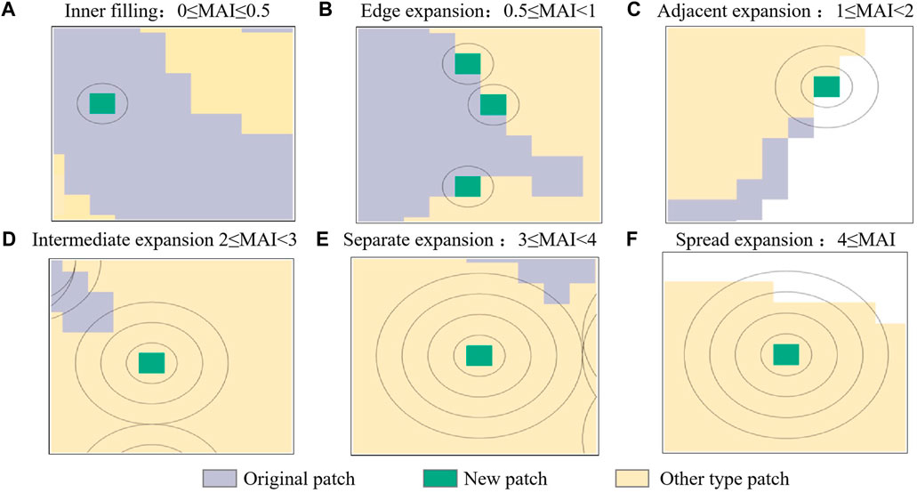
FIGURE 5. Concept map of the spatiotemporal evolution model for the vegetation restoration in the study area. Notes: Circles represent multi-stage buffering zones: (A) Inner filling; (B) Edge expansion; (C) Adjacent expansion; (D) Intermediate expansion; (E) Separate expansion; (F) Spread expansion.
3.5 Evaluation of ecological restoration effect
Landsat time-series analysis can be used to assess the effects of ecological restoration in a region. Notably, the emphasis of such an analysis should be on long- and short-term ecological restoration effects in specific areas. In this study, long- and short-term ecological restoration effects are considered according to the whole period (2000–2020) and during the disturbance–recovery cycle on the basis of LandTrendr algorithm, respectively. We used NRAs as the reference areas. The primary reason for this is that NRAs is less affected by anthropogenic activities, and its ecosystem evolution follows the natural evolution pathway, which serves our aim to effectively assess the effects of anthropogenic activity on the ecological restoration in the study area. In addition, the NRAs within the study area have the same natural conditions, e.g., climate and soil; this allowed us to assess the ecological restoration effects in the region from an objective and comparable viewpoint of ecological quality.
3.5.1 Long-term effects of ecological restoration
The DTW method is an alignment-based measurement of the similarity between two time series, and its goal is to determine the optimal alignment between the two series while ensuring minimum cost (Zhang et al., 2017). Let the reference (A{a1, a2, a3, · · ·, am}) and query (B{b1, b2, b3, · · ·, bn}) series be two time-series of lengths m and n, respectively. Here, the reference and query series are the time-series average values of the RSEI of the NRA and the time-series value of the RSEI in each pixel of the study area, respectively. The DTW distance can be calculated using Eq. 10, as follows:
where
In this study, DTW was selected because of its ability to monitor long-term ecological restoration effects. The DTW distance between the RSEI series of the study area (RSEI SA) and the time-series average values of the RSEIs in the NRA (RSEI NRA) for 2000–2022 were defined as the long-term ecological restoration effects in each pixel
where

FIGURE 6. Remote sensing ecological index (RSEI) of each area, averaged for the five natural reserve areas (NRAs), for the time-series of 2000–2022.
Note that the DTW distance was negatively related to the long-term ecological restoration effect, i.e., a lower DTW distance from the study area indicated that the pixel experienced better (high) ecological restoration effects and was evolving according to the natural evolution pathway. The DTW value between the NRA and the study area, which is the nearest distance and has a similar landform to the NAR, was calculated. The lower the
3.5.2 Short-term effects of ecological restoration
The short-term effects of ecological restoration pertain to the cycle and feedback of a disturbed ecosystem recovery process through a series of ecological programs for a specified period. In this study, we assessed the short-term effects of ecological restoration in Southern Ningxia at the onset of disturbance and the end period of the recovery process, using the RSEI derived from the LandTrendr algorithm (see Table 2). Similar to the analysis of the long-term ecological restoration effects, for the assessments of short-term effects of ecological restoration in the study area, we considered the five NRAs as the ecological reference areas. The short-term ecological restoration (
where
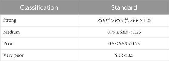
TABLE 3. Classification levels for the short-term ecological restoration effects in the study area.
4 Results
4.1 Spatiotemporal variation of ecological environmental quality
The spatial distribution of the RSEI in the study area for the 2000–2020 period is shown in Figure 7. As shown the figure, the overall ecological quality of the study area improved between 2000 and 2020. The effectiveness of the ecological management in the region was mainly manifested by an increase in the number of areas classified as “excellent,” denoting an increase from 12.4% to 31.1%; the proportion of the areas classified as “poor” decreased by 8%. The “excellent” areas were mainly distributed in the northern region of the study area. To analyze the spatiotemporal distribution of the RSEI from 2000 to 2022, the disturbance time and the time of maximum disturbance magnitude were considered (Figure 7C–F). Most of the disturbed RSEIs accounted for 20% of the total study area. Notably, 20.3% of the disturbed areas experienced only one disturbance period. The areas that experienced two RSEI disturbance periods accounted for 61.2%; 13.8% of the areas had more than four subsequent disturbance periods throughout the 22-year study period. For each maximum disturbance magnitude, we calculated the metrics that represented the occurrence date (i.e., the onset year). Figure 7D portrays the onset year of the RSEI disturbances. The disturbance onset years were split into four groups (i.e., 2001–2005, 2006–2010, 2011–2015, and 2016–2022); notably, about 60% of the primary disturbance events occurred within the first 5 years (i.e., 2000–2005). The highest magnitude of the maximum disturbance period was 0.2–0.3, with total percentage of 56.7% (Figure 7E). However, the percentage of the maximum disturbance duration was similar at each classification level, i.e., <2, 2–10, 10–18, and >18 (Figure 7F).
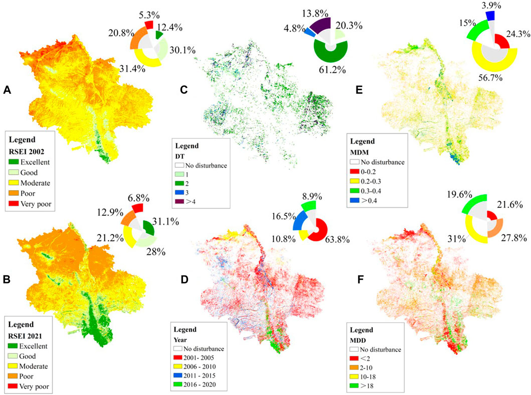
FIGURE 7. Spatiotemporal variations in the remote sensing ecological index (RSEI) from 2000 to 2022: (A) RSEI in 2000; (B) RSEI in 2022; (C) time of disturbance (DT) in RSEI; (D) Onset year of maximum disturbance magnitude; (E) maximum disturbance magnitude (MDM); and (F) maximum disturbance duration (MDD).
4.2 Spatial evolution model for vegetation restoration
In this study, forests and grasslands were considered for vegetation restoration; farmlands were excluded because they are an artificial ecological system. Our analysis revealed that the majority of areas experienced two disturbances. Therefore, the area-averaged percentages of the disturbance-onset years for the highest and second-highest disturbance magnitudes were calculated (Figure 8). As shown in the figure, the top-three area-coverage percentages were noted in 2001, 2009, and 2015. Therefore, the three time-periods, namely, 2000–2008, 2009–2014, and 2015–2022, were considered as the disturbance-recovery cycles. The spatiotemporal evolution model of vegetation restoration was analyzed in detail, shown in Figure 9. As shown the Figure 9, in spatiotemporal evolution model for 2000–2008, approximately 80% of vegetation restoration portrayed the growth pattern of “spreading expansion,” and the remaining 20% of vegetation restoration portrayed the other five patterns (i.e., edge, adjacent, intermediate, and separated expansions and inner filling). Detail statistic was shown in Table 4. During 2009–2014 and 2015–2022, the coverage area of the maximum spatiotemporal evolution model of vegetation restoration expanded. The second-maximum coverage-area value of the spatiotemporal evolution model was noted for “inner filling,” portraying an increase from 2000 to 2022, whereas spreading expansion portrayed a decrease during the same period. Overall, in the early stage, the vegetation restoration in the study area depended on artificial ecological restoration; in the present stage, it depended on a combination of natural and artificial ecological restoration.
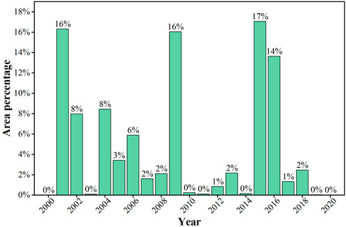
FIGURE 8. Area-averaged percentage of disturbance-onset years of the maximum and the second-maximum disturbance magnitude.
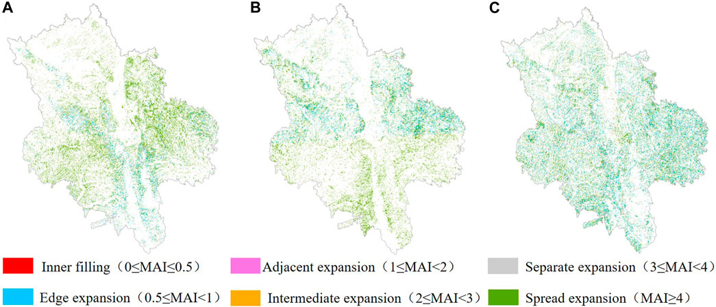
FIGURE 9. Spatiotemporal evolution model of the vegetation restoration in the study area during (A) 2000–2008; (B) 2009–2014; (C) 2015–2022.

TABLE 4. Area percentage of the spatiotemporal evolution models, based on six growth patterns (edge, adjacent, intermediate, spreading, and separated expansions and inner filling), of the vegetation restoration in the study during 2000–2008, 2009–2014, and 2015–2022.
4.3 Analysis of ecological restoration effect
4.3.1 Long-term effects of ecological restoration
The long-term effects of ecological restoration in the study area are shown in Figure 10. Figure 10A portrays the similarity in the time-series of the RSEIs of the study area and the NRAs. The areas classified as “strong” dominated the study area, mainly located in the grasslands in the northern part and around the forest area in the southern region; this pattern was similar to the observations of the NRAs (which had low anthropogenic activity). The areas classified as “medium,” “poor,” and “very poor” were located in the central part of the study area, which is a deviation of the NRA due to the effectiveness of ecological management.
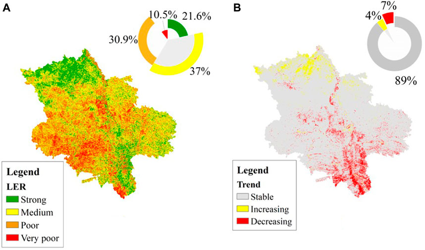
FIGURE 10. Spatiotemporal distribution of the long-term ecological restoration effects (LER) in the study area: (A) dynamic time warping (DTW) value of the remote sensing ecological indices (RSEIs) of the natural reserve area (NRAs) and the study region for 2000; (B) changing trend of the RSEI from 2000 to 2022.
We used MK tests to verify the trends in the RSEI time-series from 2000 to 2022. Figure 10B portrays the changing trend of the RSEI. The RSEI trends were classified into “increasing,” “decreasing,” and “stable” phases. The stable trends dominated the dynamic RSEI changes. Decreasing and increasing trends were observed in southern and northern regions of the study area, respectively. Notably, the majority of areas that experienced disturbances (denoted by the disturbances in the RSEI) recovered to their initial state and improved or weakened in areas affected by anthropogenic activity.
4.3.2 Short-term effects of ecological restoration
We considered four levels, namely, “very poor,” “poor,” “medium,” and “strong,” to assess the short-term ecological restoration effect (SER) in the study area; the details of the classification standard are shown in Table 3. Similar to the spatiotemporal evolution model of vegetation restoration, the cycle between disturbance onset and recovery end was considered to analyze the short-term ecological restoration effect in the study area. The spatial distribution of SER in 2000–2008, 2009–2014 and 2015–2022 is displayed in Figure 11. During 2000–2008, the area of the maximum SER was classified as “strong.” The second-maximum coverage area value of SER was “very poor;” the areas classified as “very poor” were located in the northern, southern, and eastern parts of the study area. During 2009–2014, the percentages of the “strong,” “very poor,” “medium,” and “poor” areas were 38, 23, 20, and 19%, respectively. During 2015–2022, the proportion of the coverage areas portrayed the following order: “strong,” “poor,” “very poor,” and finally “medium.” Overall, the spatiotemporal variations in the SER were obvious in all three periods. The spatial distribution of “strong” areas portrayed stability, while those of “very poor,” “poor” and “medium” areas portrayed significant variations. Notably, the negative or positive effects of SER may fluctuate depending on the degree of human interference.
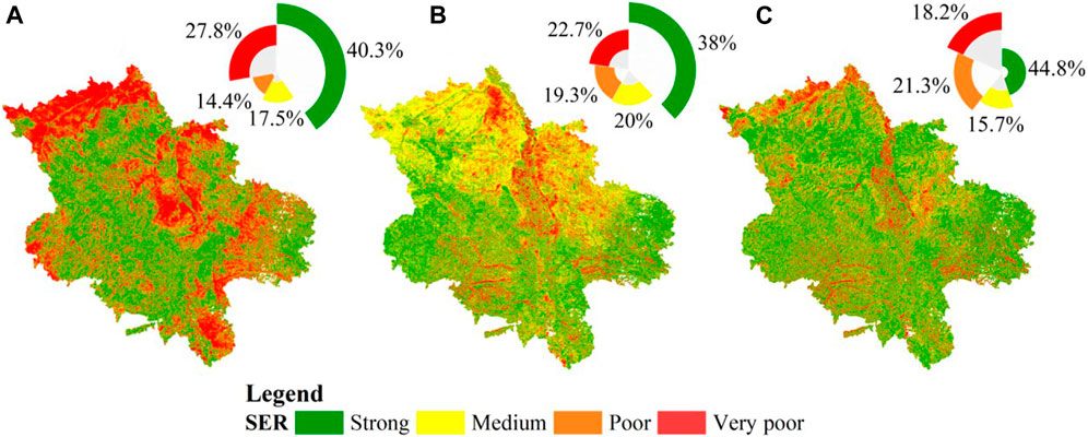
FIGURE 11. Spatial distribution of short-term ecological restoration (SER) effect in the study area in (A) 2000–2008; (B) 2009–2014; (C) 2015–2022.
5 Discussion
The RSEI has been widely used to monitor the spatial assessment of the comprehensive ecological quality of a region and conduct a dynamic analysis at a temporal scale. In the current literature, the majority of studies assess the ecological restoration effect in a region by monitoring the time-series-based changed in the RESI, while using change-detection algorithms to identify the abrupt points in a time series. To address the complexity of detecting ecological environment restoration, we introduced the MAI to quantitatively analyze the spatiotemporal change characteristics of the ecological restoration effect in the study area. Overall, from 2000 to 2022, “inner filling” portrayed an increasing tendency, while “spread expansion” portrayed a decreasing tendency, indicating that the vegetation restoration patterns occurred due to the transition from artificial restoration to a combination of artificial and natural restorations. This was indicated by the fact that newly added ecological-restoration patches filled the gaps within the pre-existing patches, reflecting the distinct restoration patterns between the effects of natural and artificial restorations. In this study, we established a comprehensive and objective ecological-assessment model for five NRAs and the study area, to evaluate the long-term effects of ecological restoration in the target region. In the future, the NRAs will be widely used to monitor the ecological restoration effects in the target study area. First, the NRAs and ecological restoration areas in the same region portrayed identical vegetation growth environments (e.g., climate conditions and soil and vegetation types) (Aronson et al., 2020), indicating that they had comparable ecological quality. Notably, NRAs can provide detailed vegetation-growth information as ideal ecological references.
This study is the first to establish a comprehensive and objective ecological-restoration assessment framework that can monitor long- and short-term ecological quality levels. In our study, DTW was introduced to reveal the long-term regional ecological restoration effect in the study area, compared to that of NRAs; this approach was used to identify the optimal path between two time-series. In addition, we considered the cycle and feedback of the recovery process of the disturbed areas for a specified period by extracting the disturbance and recovery times of the RSEI, to evaluate the short-term ecological restoration effect in the study area. This study attempts to provide a new paradigm for analyzing the ecological restoration effects in a region using long- and short-term assessment approaches.
This study has a few limitations. The majority of current studies based on RSEI involve calculating the mean value from the images captured during the growing season and then, developing image mosaics, to address the temporal instability of the RSEI during the dynamic monitoring of the ecological quality assessment of the target region (Yan et al., 2019). Owing to the complexity of natural environmental changes, multitemporal composite images are often inconsistent with real land-surface information, resulting in the misjudgment of the disturbance time in the RSEI. Furthermore, the errors in the LandTrendr algorithm parameters can affect the judgment of disturbance and recovery, leading to small-magnitude false-positive changes, poor detection, and neglecting of spatially adjacent areas (Wang et al., 2023). Moreover, climatic and seasonal differences can cause relatively large interferences in the detection of disturbance and recovery, leading to significant fluctuations in the estimations of regional vegetation and habitats (Hamunyela et al., 2020).
Overall, we developed an assessment framework to analyze the ecological restoration effects in southern Ningxia by combining the DTW method and the LandTrendr algorithm, to explore and evaluate the long- and short-term restoration effects in the region. This study extends the application of previously applied methods to different areas, while focusing on large-scale assessments of ecological restoration effects. Notably, eliminating the limitations of the proposed methods requires further exploration and optimization.
6 Conclusion
In this study, we used the RSEI, which includes the parameters of greenness, wetness, heat, and dryness, to monitor the variations in the spatiotemporal pattern of the ecological environmental quality in southern Ningxia, China. The RSEI was calculated using a yearly Landsat time-series. LandTrendr was used to analyze the disturbances in and recovery of the RSEI. Then, for different periods of discovery and recovery, we adopted the MAI to capture the expansion characteristics between the newly added and existing vegetation patches. Five NRAs were selected as the reference areas for ecological restoration in the region. The DTW value and relative index based on the time-series of the RSEIs of the study area and the NRA were analyzed to describe and quantify the long- and short-term ecological restoration effects during the study area. LandTrendr was well-suited for capturing the RSEI disturbance and recovery processes. The most important findings and conclusions of this study are as follows:
(1) The LandTrendr algorithm was successfully used for detecting the disturbance (including the times, duration, and magnitude of disturbance) and recovery in the RSEI.
(2) The ecological quality of the study area, assessed using the RSEI, portrayed significant improvement. The majority of the areas that portrayed disturbances in their RSEI values experienced two disturbance times during the entire study period; the disturbances with maximum magnitudes occurred during 2000–2005.
(3) For long-term ecological restoration effects, the areas classified as “strong” dominated the smaller the area less affected by anthropogenic activity (the southern and northern areas of the study region). For short-term ecological restoration effects, human interference has less affected the areas in the later period (2009–2014, and 2015–2022), which is classified as “strong”. The more similar were the short- and long-term ecological restoration effects to the ecological environment evolution of the NRAs.
Our study corroborates that remote sensing can provide temporally and spatially continuous synoptic observations of a region’s response to ecological quality and restoration effects. Analyzing the ecological restoration effect on long- and short-term scales can help policymakers, ecological managers, and landowners understand and improve the environmental management and vegetation status in affected areas in response to land degradation, climate change, and environmental projects.
Data availability statement
The raw data supporting the conclusion of this article will be made available by the authors, without undue reservation.
Author contributions
ZW: Data processing, Formal Analysis, Methodology, Visualization, Writing–original draft. ZA: Conceptualization, Supervision, Validation, Writing–review and editing.
Funding
The author(s) declare financial support was received for the research, authorship, and/or publication of this article. This research was funded by the Ecological Status Remote Sensing Monitoring and Assessment Project of Ningxia Province (No. 2022NCZ003508).
Conflict of interest
Authors contacted in SF case 12885576 (commercial affiliation: Beijing Feature Map Technology Co., Ltd).
Author ZW was employed by Beijing Feature Map Technology Co., Ltd.
The remaining author declares that the research was conducted in the absence of any commercial or financial relationships that could be construed as a potential conflict of interest.
Publisher’s note
All claims expressed in this article are solely those of the authors and do not necessarily represent those of their affiliated organizations, or those of the publisher, the editors and the reviewers. Any product that may be evaluated in this article, or claim that may be made by its manufacturer, is not guaranteed or endorsed by the publisher.
References
Aronson, J., Goodwin, N., Orlando, L., Eisenberg, C., and Cross, A. T. (2020). A world of possibilities: six restoration strategies to support the united nation’s decade on ecosystem restoration. Restor. Ecol. 28, 730–736. doi:10.1111/rec.13170
Boori, M. S., Choudhary, K., Paringer, R., and Kupriyanov, A. (2021). Eco-environmental quality assessment based on pressure-state-response framework by remote sensing and GIS. Remote Sens. Appl. 23, 100530. doi:10.1016/j.rsase.2021.100530
Cao, S., Zhang, L., He, Y., Zhang, Y., Chen, Y., Yao, S., et al. (2022). Effects and contributions of meteorological drought on agricultural drought under different climatic zones and vegetation types in northwest China. Sci. Total. Environ. 821, 153270. doi:10.1016/j.scitotenv.2022.153270
Chander, G., Markham, B. L., and Helder, D. L. (2009). Summary of current radiometric calibration coefficients for Landsat MSS, TM, ETM+, and EO-1 ALI sensors. Remote Sens. Environ. 113, 893–903. doi:10.1016/j.rse.2009.01.007
Czerwinski, C. J., King, D. J., and Mitchell, S. W. (2014). Mapping forest growth and decline in a temperate mixed forest using temporal trend analysis of Landsat imagery, 1987–2010. Remote Sens. Environ. 141, 188–200. doi:10.1016/j.rse.2013.11.006
Dai, X., Chen, J., and Xue, C. (2023). Spatiotemporal patterns and driving factors of the ecological environmental quality along the jakarta–bandung high-speed railway in Indonesia. Sustainability 15, 12426. doi:10.3390/su151612426
de Jong, S. M., Shen, Y., de Vries, J., Bijnaar, G., van Maanen, B., Augustinus, P., et al. (2021). Mapping mangrove dynamics and colonization patterns at the Suriname coast using historic satellite data and the LandTrendr algorithm. IJAEO 97, 102293. doi:10.1016/j.jag.2020.102293
Dong, C., Qiao, R., Yang, Z., Luo, L., and Chang, X. (2023). Eco-environmental quality assessment of the artificial oasis of Ningxia section of the yellow river with the MRSEI approach. Front. Environ. Sci. 10, 1071631. doi:10.3389/fenvs.2022.1071631
Dong, F., Pan, Y., Zhang, X., and Sun, Z. (2020). How to evaluate provincial ecological civilization construction? The case of jiangsu Province, China. Int. J. Environ. Res. Public Health 17, 5334. doi:10.3390/ijerph17155334
Gorelick, N., Hancher, M., Dixon, M., Ilyushchenko, S., Thau, D., and Moore, R. (2017). Google earth engine: planetary-scale geospatial analysis for everyone. Remote Sens. Environ. 202, 18–27. doi:10.1016/j.rse.2017.06.031
Guo, B., Wei, C., Yu, Y., Liu, Y., Li, J., Meng, C., et al. (2022). The dominant influencing factors of desertification changes in the source region of yellow river: climate change or human activity? Sci. Total. Environ. 813, 152512. doi:10.1016/j.scitotenv.2021.152512
Hamunyela, E., Brandt, P., Shirima, D., Do, H. T. T., Herold, M., and Roman-Cuesta, R. M. (2020). Space-time detection of deforestation, forest degradation and regeneration in montane forests of eastern Tanzania. IJAEO 88, 102063. doi:10.1016/j.jag.2020.102063
He, N. P., Xu, L., and He, H. L. (2020). The methods of evaluation ecosystem quality: ideal reference and key parameters. Acta Ecol. Sin. 40, 1877–1886. doi:10.5846/stxb201903150488
Hu, X., and Xu, H. (2018). A new remote sensing index for assessing the spatial heterogeneity in urban ecological quality: a case from fuzhou city, China. Ecol. Indic. 89, 11–21. doi:10.1016/j.ecolind.2018.02.006
Huang, C., Goward, S. N., Masek, J. G., Thomas, N., Zhu, Z., and Vogelmann, J. E. (2010). An automated approach for reconstructing recent forest disturbance history using dense Landsat time series stacks. Remote Sens. Environ. 114, 183–198. doi:10.1016/j.rse.2009.08.017
Ji, Q., Liang, W., Fu, B., Zhang, W., Yan, J., Lü, Y., et al. (2021). Mapping land use/cover dynamics of the yellow river basin from 1986 to 2018 supported by Google earth engine. Remote Sens. 13, 1299. doi:10.3390/rs13071299
Keogh, E. J., and Pazzani, M. J. (2001). “Derivative dynamic time warping,” in Proceedings of the 2001 SIAM International Conference on Data Mining (Chicago: SDM), 1–11. doi:10.1137/1.9781611972719
Kennedy, R. E., Yang, Z. Q., and Cohen, W. B. (2010). Detecting trends in forest disturbance and recovery using yearly landsat time series: 1. LandTrendr—temporal segmentation algorithms. Remote Sens. Environ. 114, 2897–2910. doi:10.1016/j.rse.2010.07.008
Keyantash, J. A., and Dracup, J. A. (2004). An aggregate drought index: assessing drought severity based on fluctuations in the hydrologic cycle and surface water storage. Water Resour. Res. 40. doi:10.1029/2003wr002610
Li, J., Yang, X., Jin, Y., Yang, Z., Huang, W., Zhao, L., et al. (2013). Monitoring and analysis of grassland desertification dynamics using Landsat images in Ningxia, China. Remote Sens. Environ. 138, 19–26. doi:10.1016/j.rse.2013.07.010
Li, S., Yang, S., Liu, X., Liu, Y., and Shi, M. (2015). NDVI-based analysis on the influence of climate change and human activities on vegetation restoration in the shaanxi-gansu-ningxia region, Central China. Remote Sens. 7, 11163–11182. doi:10.3390/rs70911163
Li, X., Liu, X., Hou, B., Tian, L., Yang, Q., Zhu, L., et al. (2023). Multi-dimensional evaluation of ecosystem health in China’s Loess Plateau based on function-oriented metrics and BFAST algorithm. Remote Sens. 15, 383. doi:10.3390/rs15020383
Li, Y., Cao, Z., Long, H., Liu, Y., and Li, W. (2017). Dynamic analysis of ecological environment combined with land cover and NDVI changes and implications for sustainable urban–rural development: the case of mu us sandy land, China. J. Clean. Prod. 142, 697–715. doi:10.1016/j.jclepro.2016.09.011
Liang, L., Wang, Z., and Li, J. (2019). The effect of urbanization on environmental pollution in rapidly developing urban agglomerations. J. Clean. Prod. 237, 117649. doi:10.1016/j.jclepro.2019.117649
Liu, D., Zhang, G., Li, H., Fu, Q., Li, M., Faiz, M. A., et al. (2019). Projection pursuit evaluation model of a regional surface water environment based on an ameliorative moth-flame optimization algorithm. Ecol. Indic. 107, 105674. doi:10.1016/j.ecolind.2019.105674
Liu, J., Jiao, L., Dong, T., Xu, G., Zhang, B., and Yang, L. (2018). A novel measure approach of expansion process of urban landscape: multi-order adjacency index. Sci. Geogr. Sin. 38, 1741–1749. doi:10.13249/j.cnki.sgs.2018.11.001
Liu, J., and Xu, Q. (2021). “Measurement and analysis of urban landscape expansion based on multi-order adjacency index,” in Proceedings of the 2021 IEEE 4th Advanced Information Management, Communicates, Electronic and Automation Control Conference (IMCEC), Chongqing, China, 18-20 June 2021, 967–970. doi:10.1109/imcec51613.2021.9482245
Liu, J., Xu, Q., Yi, J., and Huang, X. (2022). Analysis of the heterogeneity of urban expansion landscape patterns and driving factors based on a combined multi-order adjacency index and geodetector model. Ecol. Indic. 136, 108655. doi:10.1016/j.ecolind.2022.108655
Lu, Y., Nakicenovic, N., Visbeck, M., and Stevance, A.-S. (2015). Policy: five priorities for the UN sustainable development goals. Nature 520, 432–433. doi:10.1038/520432a
Masek, J. G., Vermote, E. F., Saleous, N. E., Wolfe, R., Hall, F. G., Huemmrich, K. F., et al. (2006). A Landsat surface reflectance dataset for north America, 1990-2000. IEEE Geosci. Remote Sens. Lett. 3, 68–72. doi:10.1109/LGRS.2005.857030
Meng, Y., Wei, C., Guo, Y., and Tang, Z. (2022). A planted forest mapping method based on long-term change trend features derived from dense Landsat time series in an ecological restoration region. Remote Sens. 14, 961. doi:10.3390/rs14040961
Nichol, J. (2005). Remote sensing of urban heat Islands by day and night. Photogramm. Eng. Rem S. 71, 613–621. doi:10.14358/PERS.71.5.613
Qiao, Y., Jiang, Y., and Zhang, C. (2021). Contribution of karst ecological restoration engineering to vegetation greening in southwest China during recent decade. Ecol. Indic. 121, 107081. doi:10.1016/j.ecolind.2020.107081
Qiu, B., Zou, F., Chen, C., Tang, Z., Zhong, J., and Yan, X. (2018). Automatic mapping afforestation, cropland reclamation and variations in cropping intensity in central east China during 2001–2016. Ecol. Indic. 91, 490–502. doi:10.1016/j.ecolind.2018.04.010
Qu, S., Wang, L., Lin, A., Yu, D., and Yuan, M. (2020). Distinguishing the impacts of climate change and anthropogenic factors on vegetation dynamics in the yangtze river basin, China. Ecol. Indic. 108, 105724. doi:10.1016/j.ecolind.2019.105724
Rhee, J., Im, J., and Carbone, G. J. (2010). Monitoring agricultural drought for arid and humid regions using multi-sensor remote sensing data. Remote Sens. Environ. 114, 2875–2887. doi:10.1016/j.rse.2010.07.005
Runge, A., Nitze, I., and Grosse, G. (2022). Remote sensing annual dynamics of rapid permafrost thaw disturbances with LandTrendr. Remote Sens. Environ. 268, 112752. doi:10.1016/j.rse.2021.112752
Shan, W., Jin, X., Ren, J., Wang, Y., Xu, Z., Fan, Y., et al. (2019). Ecological environment quality assessment based on remote sensing data for land consolidation. J. Clean. Prod. 239, 118126. doi:10.1016/j.jclepro.2019.118126
Shang, Y., Razzaq, A., Chupradit, S., An, N. B., and Abdul-Samad, Z. (2022). The role of renewable energy consumption and health expenditures in improving load capacity factor in ASEAN countries: exploring new paradigm using advance panel models. Renew. Energ. 191, 715–722. doi:10.1016/j.renene.2022.04.013
Shen, X., An, R., Feng, L., Ye, N., Zhu, L., and Li, M. (2018). Vegetation changes in the three-river headwaters region of the Tibetan plateau of China. Ecol. Indic. 93, 804–812. doi:10.1016/j.ecolind.2018.05.065
Sikder, M., Wang, C., Yao, X., Huai, X., Wu, L., KwameYeboah, F., et al. (2022). The integrated impact of GDP growth, industrialization, energy use, and urbanization on CO2 emissions in developing countries: evidence from the panel ARDL approach. Sci. Total. Environ. 837, 155795. doi:10.1016/j.scitotenv.2022.155795
Tang, Y., Liu, M., Liu, X., Wu, L., Zhao, B., and Wu, C. (2020). Spatio-temporal index based on time series of leaf area index for identifying heavy metal stress in rice under complex stressors. Int. J. Environ. Res. Public Health 17, 2265. doi:10.3390/ijerph17072265
Tian, Y., Jiang, G., Zhou, D., and Li, G. (2021). Systematically addressing the heterogeneity in the response of ecosystem services to agricultural modernization, industrialization and urbanization in the qinghai-Tibetan plateau from 2000 to 2018. J. Clean. Prod. 285, 125323. doi:10.1016/j.jclepro.2020.125323
Verbesselt, J., Hyndman, R., Newnham, G., and Culvenor, D. (2010). Detecting trend and seasonal changes in satellite image time series. Remote Sens. Environ. 114, 106–115. doi:10.1016/j.rse.2009.08.014
Wang, C., Jiang, Q., Shao, Y., Sun, S., Xiao, L., and Guo, J. (2019). Ecological environment assessment based on land use simulation: a case study in the heihe river basin. Sci. Total. Environ. 697, 133928. doi:10.1016/j.scitotenv.2019.133928
Wang, X., Ren, Y., Yu, Z., Shen, G., Cheng, H., and Tao, S. (2022). Effects of environmental factors on the distribution of microbial communities across soils and lake sediments in the hoh xil nature reserve of the qinghai-Tibetan plateau. Sci. Total. Environ. 838, 156148. doi:10.1016/j.scitotenv.2022.156148
Wang, Z., Chen, T., Zhu, D., Jia, K., and Plaza, A. (2023). RSEIFE: a new remote sensing ecological index for simulating the land surface eco-environment. J. Environ. Manag. 326, 116851. doi:10.1016/j.jenvman.2022.116851
Wei, C., Xue, X., Tian, L., Yang, Q., Hou, B., Wang, W., et al. (2023). Identification of ecological restoration approaches and effects based on the OO-ccdc algorithm in an ecologically fragile region. Remote Sens. 15, 4023. doi:10.3390/rs15164023
Xiao, W., Guo, J., He, T., Lei, K., and Deng, X. (2023). Assessing the ecological impacts of opencast coal mining in Qinghai-Tibet Plateau-a case study in Muli coal field, China. China. Ecol. Indic. 153, 110454. doi:10.1016/j.ecolind.2023.110454
Xiong, Y., Xu, W., Lu, N., Huang, S., Wu, C., Wang, L., et al. (2021). Assessment of spatial–temporal changes of ecological environment quality based on RSEI and GEE: a case study in erhai lake basin, yunnan Province, China. Ecol. Indic. 125, 107518. doi:10.1016/j.ecolind.2021.107518
Xu, H. (2013). A remote sensing index for assessment of regional ecological changes. China Environ. Sci. 33, 889–897.
Xu, X., Zhang, D., Zhang, Y., Yao, S., and Zhang, J. (2020). Evaluating the vegetation restoration potential achievement of ecological projects: a case study of yan’an, China. Land Use Pol. 90, 104293. doi:10.1016/j.landusepol.2019.104293
Yan, J., Wang, L., Song, W., Chen, Y., Chen, X., and Deng, Z. (2019). A time-series classification approach based on change detection for rapid land cover mapping. ISPRS J. Photogramm. 158, 249–262. doi:10.1016/j.isprsjprs.2019.10.003
Yang, C., Zhang, C., Li, Q., Liu, H., Gao, W., Shi, T., et al. (2020). Rapid urbanization and policy variation greatly drive ecological quality evolution in guangdong-Hong Kong-Macau greater bay area of China: a remote sensing perspective. Ecol. Indic. 115, 106373. doi:10.1016/j.ecolind.2020.106373
Yang, X., Meng, F., Fu, P., Wang, Y., and Liu, Y. (2022). Time-frequency optimization of RSEI: a case study of yangtze river basin. Ecol. Indic. 141, 109080. doi:10.1016/j.ecolind.2022.109080
Yang, Y. (2021). Evolution of habitat quality and association with land-use changes in mountainous areas: a case study of the taihang mountains in hebei Province, China. Ecol. Indic. 129, 107967. doi:10.1016/j.ecolind.2021.107967
Yi, S., Zhou, Y., Zhang, J., Li, Q., Liu, Y., Guo, Y., et al. (2023). Spatial-temporal evolution and motivation of ecological vulnerability based on RSEI and GEE in the jianghan plain from 2000 to 2020. Front. Environ. Sci. 11, 1191532. doi:10.3389/fenvs.2023.1191532
Yin, Q., Ren, Z., Wen, X., Liu, B., Song, D., Zhang, K., et al. (2023). Assessment of population genetic diversity and genetic structure of the north Chinese leopard (Panthera pardus japonensis) in fragmented habitats of the Loess Plateau, China. Glob. Ecol. Conserv. 42, e02416. doi:10.1016/j.gecco.2023.e02416
Zhang, D., Jia, Q., Xu, X., Yao, S., Chen, H., and Hou, X. (2018). Contribution of ecological policies to vegetation restoration: a case study from wuqi county in shaanxi Province, China. Land Use Pol. 73, 400–411. doi:10.1016/j.landusepol.2018.02.020
Zhang, H., Li, J., Tian, P., Pu, R., and Cao, L. (2022). Construction of ecological security patterns and ecological restoration zones in the city of ningbo, China. J. Geogr. Sci. 32, 663–681. doi:10.1007/s11442-022-1966-9
Zhang, Z., Tavenard, R., Bailly, A., Tang, X., Tang, P., and Corpetti, T. (2017). Dynamic time warping under limited warping path length. Inf. Sci. 393, 91–107. doi:10.1016/j.ins.2017.02.018
Zheng, Z., Wu, Z., Chen, Y., Guo, C., and Marinello, F. (2022). Instability of remote sensing based ecological index (RSEI) and its improvement for time series analysis. Sci. Total. Environ. 814, 152595. doi:10.1016/j.scitotenv.2021.152595
Zhou, Y., Fu, D., Lu, C., Xu, X., and Tang, Q. (2021). Positive effects of ecological restoration policies on the vegetation dynamics in a typical ecologically vulnerable area of China. Ecol. Eng. 159, 106087. doi:10.1016/j.ecoleng.2020.106087
Zhu, Z., Fu, Y., Woodcock, C. E., Olofsson, P., Vogelmann, J. E., Holden, C., et al. (2016). Including land cover change in analysis of greenness trends using all available Landsat 5, 7, and 8 images: a case study from guangzhou, China (2000–2014). Remote Sens. Environ. 185, 243–257. doi:10.1016/j.rse.2016.03.036
Zhu, Z., and Woodcock, C. E. (2014). Continuous change detection and classification of land cover using all available Landsat data. Remote Sens. Environ. 144, 152–171. doi:10.1016/j.rse.2014.01.011
Keywords: ecological environmental quality, ecological restoration effect, remote sensing ecological index (RSEI), long time-series images, natural evolution feature
Citation: Wang Z and An Z (2024) Landsat series images for evaluating ecological restoration effect from multi-time scale based on an ideal reference . Front. Environ. Sci. 12:1356269. doi: 10.3389/fenvs.2024.1356269
Received: 15 December 2023; Accepted: 21 February 2024;
Published: 12 March 2024.
Edited by:
Chengye Zhang, China University of Mining and Technology, ChinaReviewed by:
Bingyu Zhao, Beijing Normal University, ChinaBotian Zhou, Chinese Academy of Sciences (CAS), China
Jing Cui, Ministry of Emergency Management, China
Copyright © 2024 Wang and An. This is an open-access article distributed under the terms of the Creative Commons Attribution License (CC BY). The use, distribution or reproduction in other forums is permitted, provided the original author(s) and the copyright owner(s) are credited and that the original publication in this journal is cited, in accordance with accepted academic practice. No use, distribution or reproduction is permitted which does not comply with these terms.
*Correspondence: Zhihong An, YW56aGlob25nQG1haWwuY2dzLmdvdi5jbg==