Modeling soil respiration in summer maize cropland based on hyperspectral imagery and machine learning

Introduction: Soil respiration (SR), the release of carbon dioxide (CO₂) from soil due to the decomposition of organic matter and root respiration, is an important indicator for understanding agricultural carbon cycling and assessing anthropogenic impacts on the environment. Hyperspectral remote sensing offers a potential rapid, non-destructive approach for monitoring in agriculture. However, it remains uncertain whether hyperspectral remote sensing can provide an accurate and efficient method for estimating SR rate in croplands, particularly across different maize growth stages of under varying drought conditions.

Methods: In the study, we investigated the potential of combining hyperspectral remote sensing data with machine learning model (ML) to quantify SR rate in croplands. A drought field experiment was conducted, and SR and hyperspectral imagery were collected during four maize growth stages: Jointing Stage (JS), Tasseling Stage (TS), Flowering Stage (FS), and Grain Filling Stage (GFS). We compared the performance of traditional multiple linear regression (MLR) with that of an ML model (extreme gradient boosting, XGBoost), in simulating SR rate across these four growth stages.

Results: Our findings demonstrated that the simulation of the XGBoost model, utilizing soil temperature ($T_s$) and hyperspectral data, outperformed the MLR model. Across different growth stages, the SR simulated by the XGBoost model (R² = 0.8103) was more reliable than that of the MLR model (R² = 0.7451). The XGBoost model can also effectively capture the impact of drought treatments on SR.

Discussion: The XGBoost model’s tree-based structure allows it to effectively capture complex interactions and nonlinear patterns within variables, while its high sensitivity to changes in SR rates under drought conditions makes it more reliable for modeling SR across different growth stages compared to the linear-based MLR model. This study highlights the great promise of ML combined with hyperspectral imaging in predicting SR rate in croplands, which will help guide future agricultural management and environmental informatics.

1 Introduction

Soil is a vital component in the Earth’s carbon (C) cycle, playing a pivotal role in C sequestration and release on climate change (Macías and Camps Arbestain, 2010; Meena et al., 2020; Swift, 2001). Soil respiration (SR), mainly the CO₂ emissions from uplands, accounts for a significant portion of total ecosystem respiration by 60% and 90% annually. As such, SSR is the largest C resource in natural ecosystems (Yuste et al., 2005; Xu and Shang, 2016). Remarkably, the SR in croplands contributes approximately 10%–20% of the total global (Raich and Schlesinger, 1992; Sotta et al., 2004), depending on various agriculture management practices, crop types, and environmental conditions (Six et al., 2002). Additionally, cropland soil is not only a source of C emissions but also can act as a C sink through crop photosynthesis and the accumulation of soil organic matter (West and Post, 2002; Smith, 2008). Therefore, accurate monitoring and estimation of SR in croplands are crucial for understanding the complex dynamics of terrestrial C cycles, which are increasingly influenced by human actives.

Many approaches are currently used to monitor and estimate SR in croplands. The main field monitoring methods include the static chamber method (Rochette et al., 1992), dynamic chamber method (Rochette et al., 1997), and micrometeorological method (Van Cleve et al., 1979; Pete et al., 2010). However, these approaches have certain limitations, such as: 1) insufficient representation due to limited observations of spatial heterogeneity (Liu et al., 2016), and 2) an inability to capture regional patterns influenced by varying agricultural practices, land-use changes, and other management activities (Chen et al., 2020; Ramesh et al., 2019). Recently, hyperspectral remote sensing has been widely used, as it can capture detailed spectral information across a wide range of wavelengths, enabling precise assessment of various soil and vegetation parameters (Yu et al., 2020; Teke et al., 2013). For example, wavelengths around 1,400 nm and 1,900 nm are effective for detecting soil moisture due to water absorption features, while 680 nm (red) and 750–800 nm (near-infrared) are commonly used to assess chlorophyll content and plant health (Lobell and Asner, 2002; Tucker, 1979).Hyperspectral remote sensing offers a promising way for more accurate and efficient monitoring of agricultural ecosystems (Singh and Babu, 2022), which is crucial for sustainable agriculture and environmental conservation. However, due to the large volume of hyperspectral data, challenges arise in efficiently processing, analyzing, and interpreting this data using traditional methods (Bioucas-Dias et al., 2013; Liang et al., 2020). For example, traditional statistical models often struggle to handle the high dimensionality of hyperspectral data, leading to overfitting or poor generalization (Ullah et al., 2024). Moreover, these statistical methods typically involve manual feature selection, making the processes both labor-intensive and susceptible to human error (Hastie et al., 2009; Feng et al., 2015).

Recently, the integration of machine learning (ML) has advanced the applications of hyperspectral remote sensing (Guerri et al., 2024; Le et al., 2020). For example, ML is capable of managing large datasets and revealing intricate relationships between hyperspectral variables (Burger and Gowen, 2011). Many ML algorithms, such as Artificial Neural Networks (ANN), Random Forest (RF), Support Vector Machines (SVM), and Extreme Gradient Boosting (XGBoost), have been extensively utilized to estimate agricultural indicators, such as leaf nitrogen content (Yamashita et al., 2020), leaf chlorophyll content (Wang et al., 2020; An et al., 2020), and soil moisture content (Tang et al., 2023) etc., very well. Moreover, the integration of special ML algorithms with hyperspectral remote sensing can also enhance the analytical efficiency of hyperspectral data. For instance, as a boosting-based ensemble learning method capable of handling both regression and classification problems, the XGBoost features parallel and distributed computing capabilities, making it to be one of the fastest and most efficient decision tree algorithms (Ma et al., 2021). However, the application of hyperspectral data with XGBoost model has not been well examined in estimating SR rate in croplands.

Hence, this study seeks to investigate the capabilities of hyperspectral remote sensing in monitoring SR in maize croplands through different modeling approaches. Based on the observations of the SR, hyperspectral parameters and climate factors in the summer maize cultivation, we established two different SR models of the summer maize cropland, using traditional multiple linear regression (MLR) and ML XGBoost. We examined their modeling performances on the accuracy of simulated SR across different growth stages and drought treatments. The simulated and measured relationship between the SR and soil temperature ($T_s$) were also analyzed. The study can contribute to the dynamic monitoring and simulation of SR in agricultural ecosystems with hyperspectral remote sensing, and benefit soil health management and agricultural sustainability under global climate change.

2 Materials and methods

2.1 Study site

Shandong province is the main critical grain-producing area in China, characterized by maize is one of the main grain crops in the province. The experiment was conducted at the Agricultural Water Resource Efficient Use Experimental Site of Ludong University (37.54° N, 121.39° E) in the province. The elevation of the site is 47.8 m. The region experiences a warm temperate continental monsoon climate, with mean annual temperature ranging from 11.8°C to 13.0°C, and annual precipitation varying between 651.9 mm and 722.2 mm (mainly occurring in July and August) (Yantai Meteorological Bureau, 2023). The soil is loam, with pH value of 6.5–7.0, organic matter content ranging from 1.5% to 2.5%, organic C content between 1.0% and 1.5%, and nitrogen content ranging from 0.05% to 0.15% (Chen et al., 2019). The maximum field water holding capacity of the soil is about 22% (Zhang et al., 2021).

2.2 Experimental design

The summer maize cultivar “Jinhai No. 5” was sown in pots on 11 June 2023 and harvested on 27 September 2023. We conducted drought experiments during four different growth stages of maize: Jointing Stage (JS), Tasseling Stage (TS), Flowering Stage (FS), Grain Filling Stage (GFS). During each drought period, the soil moisture of control treatment was maintained at 60%–70% of the maximum field capacity, while the drought treatment was maintained at 40%–50% of the maximum field capacity. Each treatment was replicated in three pots, resulting in a total of 15 potted plants (4 drought-period treatments × 3 replicates + 1 control treatment × 3 replicates) (Figure 1). The pots used for the maize were plastic containers weighing 1.4 kg, with an upper diameter of 43 cm, a bottom diameter of 26 cm, and a height of 24 cm (Figure 1). Each pots was filled with a mixture of 20 kg of soil from the site and 5 g of “Sackoff” compound fertilizer (total nutrient content of 51.0%). Soil moisture of all treatments was monitored and maintained daily between 17:00 and 18:00 by weighting the pots. During watering, the pots were placed on an electronic scale to ensure precise control of water application, allowing for accurate adjustments as necessary.

Figure 1

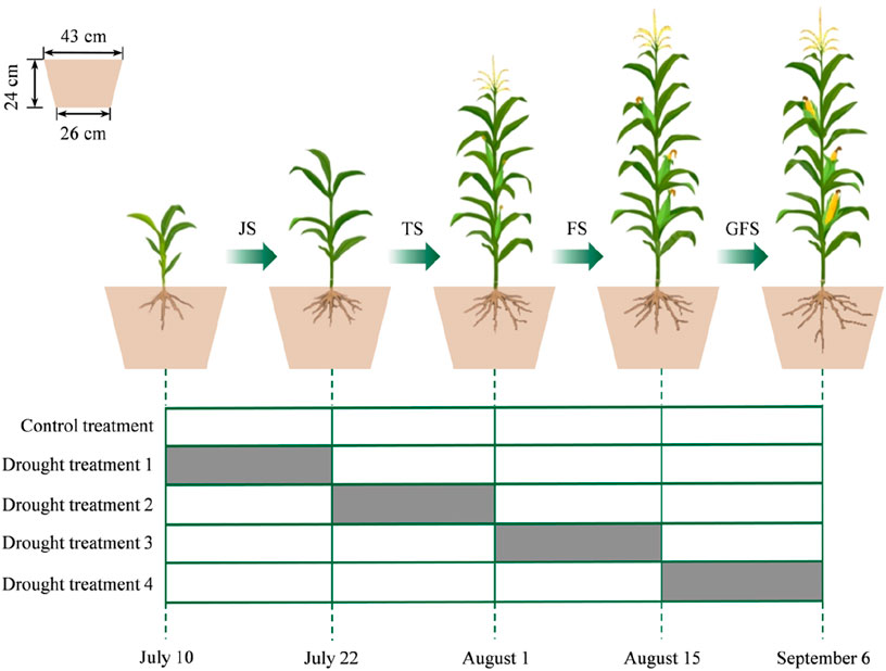
Figure 1. Schematic diagram of the experimental design of summer maize across different growth stages (JS, TS, FS, GFS). JS: Jointing Stage, TS: Tasseling Stage, FS: Flowering Stage, GFS: Grain Filling Stage. The green arrows indicate the progression of this growth stage. The grey bars represent the drought treatments applied during the corresponding growth stages, while the blank bars represent the control treatment. The dates in the figure represents the time when >75% of the maize had reached the specific growth stage.

2.3 Soil measurement

SR rates were measured using the Photosynthesis-Fluorescence System (LI-6400XT, LI-COR Biosciences, Lincoln, NE, United States) equipped with the 6400–09 SR Chamber. The SR measurement collar was installed in each pot to a depth of 3 cm and 2 cm above the soil surface, with a measurement surface area of 80 cm². There was a 24-hour waiting period between the placement of the ring and the first SR monitoring. The $T_s$ was measured using the soil temperature sensor (equipped with LI-6400-09) during SR measurements, with the sensor inserted near the SR measurement point at a depth of 5–10 cm. SR and $T_s$ were measured simultaneously for all pots to ensure consistency across the experiment.

To estimate the dependence of seasonal variations in SR on $T_s$, the relationship was fitted using an exponential equation (Equation 1):

$SR=k{e}^{a{T}_s}(1)$

Where the unit of SR is μmol·m⁻²·s⁻¹, the unit of $T_s$ is ◦C, and k and a are constants (Davidson et al., 1998; Knohl et al., 2008). The temperature sensitivity of SR, represented by Q₁₀, which indicates the increase in SR for every 10°C rise in temperature, was calculated using Equation 2:

$Q_{10}=e^{10a}(2)$

2.4 Hyperspectral measurement and data processing

Hyperspectral data for summer maize were collected using a spectrometer (ASD FieldSpec HandHeld2) between 11:00 a.m. and 1:00 p.m. under clear skies with minimal wind to ensure consistency. The spectrometer was calibrated with a standard reference panel to approximate 100% reflectance. During each measurement, the spectrometer was held 10–15 cm above the maize canopy, with ten readings averaged. In this study, spectral data from 350 to 910 nm were used (Table 1). For example, wavelengths of 680 nm and 800 nm were used to calculate Normalized Difference Vegetation Index (NDVI), while 705 nm and 750 nm were used to calculate NDVI₇₀₅ (Table 1). These hyperspectral vegetation indices are important indicators of plant health, biomass, and stress levels, providing critical information for monitoring crop conditions. They help assess photosynthetic activity and water content of vegetation, both of which are essential for evaluating crop performance and SR dynamics. Triangular parameters, such as edge amplitudes and areas (e.g., blue, yellow, red edges), are often used to represent spectral shifts related to changes in vegetation physiology, including pigment concentration, stress response, and overall growth status (Table 1).

Table 1

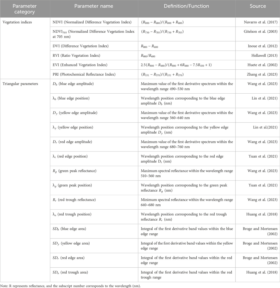
Table 1. The hyperspectral parameters used in this study.

2.5 Modeling approach

2.5.1 Multiple linear regression

Multiple linear regression (MLR) is a traditional statistical technique used to model the relationship between a dependent variable and two or more independent variables, assuming a linear association. Due to its computational simplicity and strong explanatory power, MLR is widely applied in hyperspectral inversion studies of crop indices (Ma et al., 2023). In this study, SR was the dependent variable, while key hyperspectral parameters, along with climate factors such as $T_s$, were the independent variables. The final optimal model was selected using the Akaike Information Criterion (AIC) (Vrieze, 2012).

The MLR model can be represented as Equation 3:

$y_i={\beta }_0+{\beta }_1{x}_1+{\beta }_2{x}_2+\dots +{\beta }_n{x}_n+ϵ(3)$

Where, $y_i$ represents the SR in this study, ${\beta }_0$ is the intercept, ${\beta }_1$, ${\beta }_2$, … ${\beta }_n$ are the regression coefficients for the input parameters $x_1$, $x_2$, … $x_n$; $x_1$, $x_2$, … $x_n$ are the key hyperspectral parameters and $T_s$ listed in Table 1, $ϵ$ is the error term.

The MLR model was developed using MATLAB (version 2022a, Math Works, Natick, MA, United States) with the Statistics and ML Toolbox. AIC was employed for variable selection, iterating through all parameter combinations to identify the subset that minimized AIC values, which yielded the final optimal model. The model’s performance was evaluated using the “fitlm” function, with AIC calculated based on the residual sum of squares. The coefficients of the best-performing model were standardized to assess each predictor’s contribution to SR, and these contributions were visualized in a bar chart. During AIC selection, all results were systematically documented, providing a comprehensive overview of the final optimal MLR model’s performance and variable contributions.

2.5.2 Machine learning model

XGBoost, an advanced gradient boosting algorithm, is composed of K CART trees and can be represented by the following Equation 4:

$\mathrm{\Phi }\left(x_i\right)={\displaystyle \sum _{k=1}^K}{f}_k\left(x_i\right),f_k\in F(4)$

Here, $f_k$ represents the kth tree, $f_k\left(x_i\right)$ the score of the ith node of the kth tree, and $F$ is the collection of all conceivable CART trees, defined as $F=\left\{f|f\left(x\right)=w_{q\left(x\right)}\right\}$, where $w_{q\left(x\right)}$ is the weight vector comprising the leaf node weights in the regression tree.

Like many ML algorithms, XGBoost includes a loss function to measure model accuracy, paired with a regularization term to control model complexity and prevent overfitting. The complete objective function L is defined as Equation 5:

$L\left(\mathrm{\Phi }\right)=l\left(y_i,\widehat{y_i}\right)+{\displaystyle \sum _{k=1}^K}\mathrm{\Omega }\left(f_k\right)(5)$

In this equation, $l$ is the loss function, measuring the difference between predicted values ($\widehat{y_i}$) and the actual targets ($y_i$), while $\mathrm{\Omega }$ represents the regularization term, detailed as Equation 6:

$\mathrm{\Omega }\left(f\right)=\gamma T+\frac{1}{2}\lambda {‖\omega ‖}^2(6)$

Here, $\gamma$ quantifies the complexity of the tree’s leaves; $T$ is the number of leaves; $\lambda$ controls the penalty; and $\omega$ represents the leaf node scores (Ma et al., 2021).

The XGBoost model was implemented using the ‘xgboost’ package in R (version x64 4.0.4), with the following parameters: the objective function was “reg: squarederror,” the evaluation metric was root mean square error (RMSE), the learning rate was 0.1, the maximum tree depth was 6, and both data and feature subsampling ratios were set to 0.7. The XGBoost model was trained over 100 iterations, and performance was assessed using the coefficient of determination (R²) and RMSE. After model training, feature importance was evaluated using the ‘xgb.importance’ function. All results were systematically documented and exported for further analysis, providing a comprehensive view of the XGBoost model’s performance.

2.5.3 Statistical analysis

Statistical analysis was primarily conducted using SPSS software (version 22, IBM Corp., Armonk, NY, United States), and all figures were generated using R (version x64 4.0.4; R Core Team, Vienna, Austria) to ensure high-quality visualization. Descriptive statistics were computed to summarize the sample characteristics, and independent sample t-tests were used to assess differences between groups a, b, and c. A significance level of 0.05 was set, with p < 0.05 considered statistically significant.

Pearson correlation analysis was conducted in R using the ‘cor()’ function to calculate the Pearson correlation coefficients. Additionally, a correlation matrix plot was generated using the “PerformanceAnalytics” package in R to visually represent the relationships between variables.

A randomly selected 1/3 samples set was used to validate the reliability and robustness of all models. To assess the accuracy of SR simulations produced by the MLR and XGBoost models, we applied three key evaluation metrics: the coefficient of determination (R²), root mean square error (RMSE) and residual. R² indicates how well the model predictions explain the variability in observed SR values. A higher R² value suggests that the model captures more of the data’s variability, with values closer to 1 indicating stronger predictive accuracy. The RMSE quantifies the average magnitude of the error between predicted and observed SR values, with lower values indicating better model performance. The residuals were computed as the difference between the observed and predicted values of SR. Their equations (Equations 7–9) are as follows:

$R^2=1-\frac{{\displaystyle \sum _{i=1}^n}{\left(y_i-p\left(x_i\right)\right)}^2}{{{\displaystyle \sum _{i=1}^n}\left(y_i-{\overline{y}}_i\right)}^2}(7)$

$RMSE=\sqrt{\frac{1}{n}{\displaystyle \sum _{i=1}^n}{\left(p\left(x_i\right)-y_i\right)}^2}(8)$

${Residual}_i={Observed}_i-{Predicted}_i(9)$

Where $n$ represents the number of samples in the predictive set; $p\left(x_i\right)$ represents the simulated values, and $y_i$ represents the measured value; ${Observed}_i$ is the observational SR rate for the ith sample; ${Predicted}_i$ is the predicted SR rate for the i-th sample.

3 Results

3.1 Model evaluation for the whole growth season

Figure 2 showed the importance of input features in both the XGBoost and MLR models, along with their contributions to simulating SR. In the XGBoost model (Figure 2A), the feature $T_s$ was the most significant factor, suggesting that soil temperature $T_s$ had the largest influence on SR predictions for summer maize. Other important features included the red edge position (${\lambda }_r$) and red trough reflectance ($R_r$). In contrast, the MLR model (Figure 2B), which was optimized using the AIC (AIC = −68.3913), revealed that the Ratio Vegetation Index (RVI) had the greatest impact. This finding suggests that specific vegetation indices played a critical explanatory role in the MLR model’s simulation of SR. Additional features, such as the NDVI and the Photochemical Reflectance Index (PRI), also had significant effects on the MLR model’s performance.

Figure 2

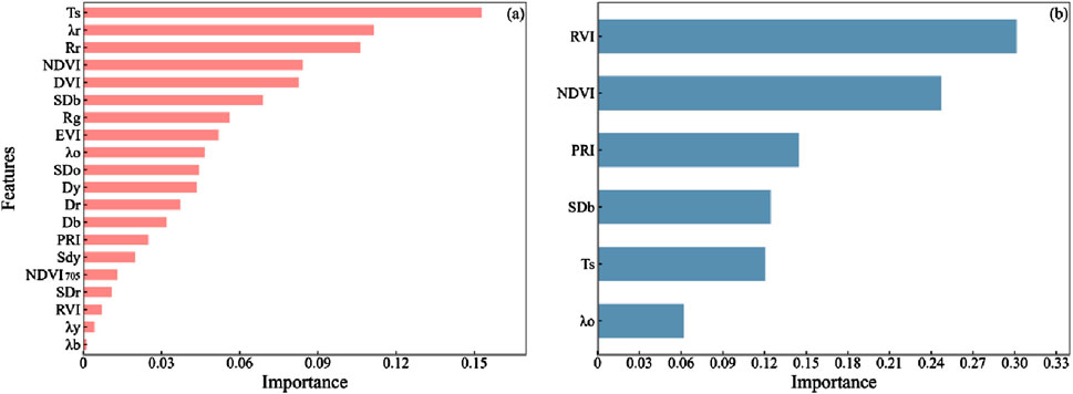
Figure 2. Parameter contributions of the MLR and XGBoost models. (A) MLR; (B) XGBoost. The parameters full names see Table 1.

The XGBoost model significantly outperformed the MLR model in estimating SR for summer maize throughout the whole growth season (Figure 3A). The XGBoost model achieved a higher R² value (R² = 0.9298), indicating a stronger ability to explain variance, and a lower RMSE (RMSE = 0.2887), demonstrating lower prediction error. The fitted curve for the XGBoost model closely aligned with the 1:1 line, with data points clustered around it, suggesting that the XGBoost model accurately simulated SR across both high and low values. In contrast, the MLR model’s fitted curve deviated more from the 1:1 line, with data points showing greater scatter. The MLR model tended to overestimate lower SR values and underestimate higher SR values.

Figure 3

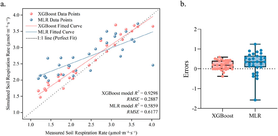
Figure 3. Different behaviors of MLR and XGBoost models in simulating soil respiration rate (A). Relationships between soil respiration measurements and simulations by the MLR and XGBoost models for the whole growth season (n = 30) (B). Comparison of residual error distributions for XGBoost and MLR models (n = 30).

In the comparative analysis of model errors, the residual distributions of the XGBoost and MLR models exhibited significant differences (Figure 3B). The error of the XGBoost model was smaller and more concentrated, with residuals primarily ranging between −1 and 1, and a median close to 0, indicating that XGBoost demonstrated higher accuracy and stability in its prediction of SR rate. In contrast, the error range of the MLR model was broader, spanning from −2 to 2, with notably higher variability in the residuals. The boxplot of the MLR model displayed a wider interquartile range and pronounced lower outliers, suggesting that this model yielded larger errors for certain data points and lacked stability in its predictions.

3.2 Comparison of simulated SR under different treatment conditions

As shown in Figure 4, both the MLR and XGBoost models successfully captured the effects of drought on SR rates, indicating that SR rates decreased under drought treatments across all growth stages (JS, TS, FS, and GFS). However, the XGBoost model performed better than the MLR model, with its simulated values more closely aligning with the measured values, particularly under the control treatment across all four stages. In contrast, the MLR model exhibited significant discrepancies between its simulated and measured values, especially during drought treatments.

Figure 4

Figure 4. Comparison of measured and simulated soil respiration rates by the MLR and XGBoost models across the four growth stages under different treatment conditions. (A) Control treatment; (B) Drought treatment. JS: Jointing Stage, TS: Tasseling Stage, FS: Flowering Stage, GFS: Grain Filling Stage. Values with different letters (A–C) indicate significant differences between the model simulations and the measured values (p < 0.05).

The performances of both models in simulating SR rates for summer maize varied across different treatments and growth stages. Under control treatment, the XGBoost model more accurately simulated SR rates, though it slight overestimated them by approximately 5.6% during the JS. In contrast, the MLR model consistently underestimated SR rates across all growth stages, with the most significant underestimation occurred during the JS (15.35%), and the least during the FS (7.32%). Under drought treatments, both models significantly overestimated SR rates across all stages. However, the MLR model’s overestimations were much larger than those of the XGBoost model. The MLR model overestimated SR rates by 87.25% during the JS, with the highest error occurring under drought treatments, while the smallest overestimation occurred during the GFS (4.54%). Although the XGBoost model also overestimated SR rates at all stages, its errors were much smaller, with the largest overestimation occurring during the JS stage (40.1%) and the smallest during the GFS stage (14.6%). These results indicate the superior performance of the XGBoost model in modeling SR under varying moisture conditions.

3.3 Comparison of measured and simulated relationships between SR and ${\mathit{T}}_{\mathit{s}}$

The sensitivity of SR rates to $T_s$ varied between the MLR and XGBoost models (Figure 5). Both models reasonably captured the relationship of $T_s$ on SR, as evidenced by their fitted curves aligning with the observed data points. However, the sensitivity of the simulated SR values to temperature (Q₁₀) decreased in both control and drought treatments. Despite this, the XGBoost model generally outperformed the MLR model. Under control treatments, the sensitivity coefficient of SR rates to $T_s$ simulated by the XGBoost model (Q₁₀ = 1.3418), was only 6.1% lower than the measured sensitivity coefficient (Q₁₀ = 1.4287). In contrast, the MLR model’s sensitivity coefficient (Q₁₀ = 1.1888) showed a more substantial decrease of 16.79%. Additionally, both models exhibited reduced explanatory power in their fitted functions, suggesting that discrepancies between simulated and measured values affected the Q₁₀ values. Nevertheless, the XGBoost model (R² = 0.6584) provided better explanatory power than the MLR model (R² = 0.6528). Under drought treatments, the XGBoost model’s sensitivity coefficient (Q₁₀ = 1.1208) was 4.49% lower than the measured coefficient (Q₁₀ = 1.1735), while the MLR model’s coefficient (Q₁₀ = 1.0544) decreased by 20.48%. Although both models showed reduced explanatory power for SR variability under drought conditions, the Q₁₀ values from the fitted functions in both models indicated higher explanatory power than the measured values.

Figure 5

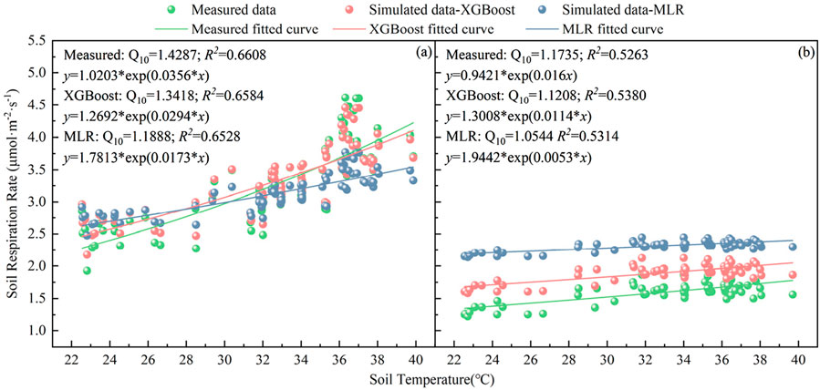
Figure 5. Comparison on the measured and simulated relationships between soil respiration and temperature. (A) Control treatment, (B) Drought treatment.

4 Discussion

4.1 Model performance comparison

In this study, we compared the performance of the MLR and XGBoost models in simulating SR across different growth stages under both drought and control treatments. The results consistently demonstrated that the XGBoost model outperformed the MLR model, as indicated by its higher R² and lower RMSE values. The superior performance of the XGBoost model is primarily attributed to its ability to capture non-linear relationships between parameters (Chen and Guestrin, 2016; Ding, 2024).

A Pearson correlation analysis was conducted to examine the relationships between various parameters and SR (Figure 6). The analysis revealed that parameters, such as ${\mathrm{D}}_{\mathrm{b}}$, ${\mathrm{D}}_{\mathrm{r}}$, DVI, EVI, $R_g$, $R_r$, ${SD}_b$, ${SD}_r$, ${SD}_y$ and $T_s,$ exhibited clear nonlinear trends with SR, indicating that the response of SR to these parameters is not uniform but varies in intensity depending on other parameters. In contrast, parameters, such as ${\lambda }_b$, ${\lambda }_g$, and ${\lambda }_y$, showed weak linear relationships with SR, with their correlations being statistically insignificant. This indicates that, while some parameters may exhibit linear relationships with SR, their overall contribution to SR variability is minimal.

Figure 6

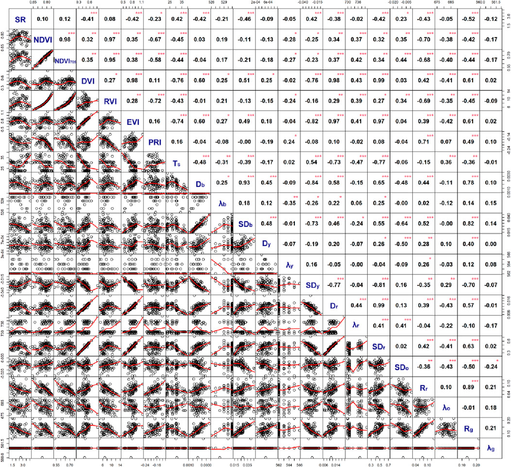
Figure 6. The correlation matrix of soil respiration and all parameters. Below the diagonal, bivariate scatter plots with a red fitted line representing the relationship between the two parameters are displayed. Above the diagonal, the correlation values along with significance levels indicated by stars are shown. *Represents a significant difference at 0.01 < p ≤ 0.05; **represents a significant difference at 0.005 < p ≤ 0.01; ***represents a significant difference at p ≤ 0.005. Each parameter is displayed as a blue label on the diagonal, and the full names of the parameters are provided in Table 1.

The XGBoost, a decision tree-based gradient boosting framework, excels at handling non-linear relationships (Chen and Guestrin, 2016; Liang et al., 2020; Nabavi et al., 2023). The decision trees in the XGBoost model divide data into distinct regions, enabling the model to capture complex interactions. The XGBoost model builds these tree models incrementally, using a boosting method where each new tree corrects the errors of the previous one (Kiangala and Wang, 2021; Zhang et al., 2019). This recursive process allows the XGBoost model to capture intricate patterns and non-linear features in the data, whereas the traditional MLR model struggles due to its inherent linear assumptions. For instance, parameters like $T_s$ and $D_b$, which showed high non-linearity with the SR rate (Figure 6), were better captured by the XGBoost model, while the MLR model failed to account for their non-linear impacts.

Additionally, the XGBoost model handles multicollinearity among parameters effectively (Chen et al., 2022). Its tree-based structure prioritizes important features during model construction without being limited by linear relationships (Kern et al., 2019; Tong et al., 2003). This ensures strong predictive performance even in the presence of highly correlated variables. For example, in this study, significant multicollinearity existed among parameters, such as NDVI, PRI, and $T_s$, which posed challenges for the traditional MLR model (Garg and Tai, 2013). Since the MLR model assumes that predictor variables are independent, it struggles with stability and reliability when dealing with multicollinearity (Weaving et al., 2019; Chan et al., 2022). While the MLR model used AIC to select important predictors, including NDVI, RVI, PRI, $T_s$, and ${SD}_b$, it still struggled to manage the effects of multicollinearity, resulting in weaker performance. In contrast, XGBoost automatically accounts for variable interactions in each decision tree split, mitigating the negative effects of multicollinearity on model performance (Kavzoglu and Teke, 2022; Wu et al., 2024).

The XGBoost model stands out in identifying and leveraging feature interactions, making it suitable for complex, high-dimensional datasets (Hastie et al., 2009; Huang et al., 2022). Unlike MLR, which relies on predefined linear relationships and manually added interaction terms, XGBoost dynamically uncovers important feature interactions during training (Niazkar et al., 2024). This enables XGBoost to capture non-linear and higher-order interactions directly from the data, without the need for explicit feature engineering (Weaving et al., 2019). In contrast, MLR requires prior assumptions about feature interactions, which increases the risk of inaccuracies when dealing with complex variable interdependencies.

Furthermore, the XGBoost model also uses Lasso and Ridge regularization techniques to prevent overfitting, enhancing its modeling robustness (Friedman, 2001; Elavarasan and Vincent, 2020). Regularization penalizes overly complex models, allowing the XGBoost model to maintain strong performance even in noisy datasets or when faced with low-importance variables (Zhang and Jánošík, 2024). In contrast, the traditional MLR model, lacking these regularization treatments, is more vulnerable to overfitting, especially in the presence of multicollinearity (Dormann et al., 2013). Although AIC helps select optimal predictors in the MLR model, it does not fully mitigate the risk of overfitting, particularly when dealing with correlated variables or when the model becomes too complex. Hence, the XGBoost model’s ability to manage data complexity more effectively through regularization offers a clear advantage over the MLR model.

In summary, the XGBoost model’s ability to capture non-linear relationships, manage multicollinearity, and utilize regularization techniques significantly enhances its robustness and predictive accuracy. In contrast, the MLR model’s reliance on linear assumptions and vulnerability to overfitting limit its effectiveness when applied to complex datasets. Our study underscores the importance of selecting appropriate modeling techniques tailored to the complex and non-linear nature of ecological and agricultural data.

4.2 Changes of soil respiration rate with hyperspectral features

This study utilized hyperspectral remote sensing features to predict SR in summer maize, demonstrating the potential of hyperspectral data for non-destructive SR estimation. The correlation between SR and hyperspectral features arrised from the hyperspectral data’s ability to indirectly capture key vegetation and soil characteristics, which reflect key environmental and biological factors that influencing SR (Huang et al., 2014). Previous research has shown that hyperspectral data can indicate SR indirectly through vegetation indices, chlorophyll content, soil surface reflectance, and other spectral parameters (Cicuendez et al., 2015; Ding et al., 2021). These features are closely related to plant growth, soil moisture, and temperature conditions, all of which directly impact root respiration and microbial activity, thereby driving SR.

In prior studies, hyperspectral remote sensing has represented SR effectively by capturing vegetation spectral characteristics, such as chlorophyll concentration and biomass content, that are closely tied to plant productivity and photosynthetic activity (Ding et al., 2021). These processes influence root and microbial respiration, which in turn affect SR (Feilhauer et al., 2017). Additionally, hyperspectral data are sensitive to soil and plant water content, which can indicate SR fluctuations by revealing variation in soil moisture that influence SR rate. By analyzing specific spectral bands and indices, such as NDVI and chlorophyll-based indices, hyperspectral data can capture those plant and soil health indicators relevant to SR, thus enhancing the estimation accuracy of SR models (Ding et al., 2021; Yao et al., 2021).

However, several environmental and biological factors significantly influence the relationship between SR and hyperspectral data. For example, plant species and growth stage have key influence on spectral characteristics, as they show substantial variability in physiological responses, canopy structure, and leaf biochemistry, all of which alter spectral signatures (Feilhauer et al., 2017). Water condition directly impacts SR by affecting microbial activity and root respiration, which drive variation in SR rate (Philippot et al., 2024). Hyperspectral data, especially water absorption bands, can indirectly capture this influence on SR. Moreover, soil temperature is another significant factor. Higher temperatures tend to promote microbial and root respiration, and temperature changes influence vegetation spectral response, which in turn affects SR estimate derived from hyperspectral data (Yao et al., 2021).

Our findings align with some previously observed trends, though differences also exist. Similar to other studies, we found that specific vegetation indices (e.g., NDVI) effectively capture SR changes across different growth stages, indicating that hyperspectral data are robust in reflecting plant-soil interactions that drive SR (Cicuendez et al., 2015). However, the sensitivities of SR to drought treatments and growth stage variation are more pronounced in our study. These differences may arise from our experimental conditions, including maize growth stages under controlled drought treatments, as well as the local climate and soil properties differing from those in other studies.

4.3 Uncertainties and future work

Although we found that the performance of ML XGBoost model in simulating SR rates during the growth stages of maize cropland was better than the traditional MLR model, there are still some uncertainties in the study. One limitation is the absence of continuous drought treatments across all four growth stages (JS, TS, SS, and GFS). While the current experimental design provides insights into short-term SR responses, long-term drought exposure could induce more complex responses, potentially altering microbial activity, root respiration, and C cycling over time (Wang et al., 2014). Hence, future studies incorporating continuous drought treatments throughout all growth stages would be valuable for comprehensively assessing the long-term impacts of water stress on SR through ML models.

Further modelling research is needed to examine the effects of initiating drought during different growth stages. The timing of drought onset is crucial, as SR responses can vary depending on the developmental stage of the crop. For instance, early-stage drought may have a more pronounced effect on root development and microbial interactions, while drought at later stages may alter C allocation and respiration processes (Liu et al., 2022). Additional field and modeling experiments applying drought treatments at varying growth stages over extended periods would provide more robust estimates of SR dynamics, particularly when using hyperspectral remote sensing under varying environmental stress scenarios (Zhang et al., 2019).

Finally, this study was conducted with maize grown in potted plants, which may not fully represent the complexities of field conditions. Factors such as soil texture, microclimate, and micrograph, etc., could also influence SR (Conant et al., 2000). Therefore, future large-scale field experiments are necessary to strengthen the evaluation of the ML models using hyperspectral remote sensing in more complex, real-world conditions. These studies would provide a more realistic assessment of SR under various drought conditions and enhance the robustness of the conclusions drawn from this research.

5 Conclusion

This study compared the performance of traditional MLR and ML XGBoost models in simulating SR rates of summer maize under different growth stages and drought treatment conditions. The results clearly demonstrate that the XGBoost model significantly outperformed the MLR model in both accuracy and predictive capability, effectively capturing the variability in SR rates across the different stages. Moreover, the XGBoost model demonstrated superior sensitivity to soil temperature compared to the MLR model. Our findings suggest that the ML XGBoost model, when combined with hyperspectral remote sensing, provides a robust tool for simulating SR in summer maize croplands under varying environmental conditions. This highlights the potential of integrating ML and hyperspectral remote sensing as a promising approach for modeling C cycling in croplands.

Data availability statement

The raw data supporting the conclusions of this article will be made available by the authors, without undue reservation.

Author contributions

FZ: Data curation, Methodology, Writing–original draft. JS: Writing–review and editing. HZ: Methodology, Writing–review and editing. LY: Methodology, Writing–review and editing. XZ: Data curation, Writing–review and editing. JZ: Writing–review and editing. XB: Writing–review and editing. YC: Writing–review and editing. FuY: Funding acquisition, Project administration, Writing–review and editing. FeY: Conceptualization, Supervision, Writing–original draft, Writing–review and editing.

Funding

The author(s) declare that financial support was received for the research, authorship, and/or publication of this article. This study was partially supported by the National Natural Science Foundation of China (51809284 and 51309016), the National Key Research and Development Program of China (2016YFC0400206-04), the Shandong Provincial Natural Science Foundation (ZR2020ME254 and ZR2020QDO61), the Young Scientists Innovation Fund of State Key Laboratory of Black Soils Conservation and Utilization (2023HTDGZ-QN-03), and the Innovation and Entrepreneurship Talent Fund of Jilin Province.

Acknowledgments

We thank Fengjuan Che from Shandong Normal University and Wenzheng Yao from Shandong Sport University for their invaluable support during the field experiment.

Conflict of interest

The authors declare that the research was conducted in the absence of any commercial or financial relationships that could be construed as a potential conflict of interest.

The author(s) declared that they were an editorial board member of Frontiers, at the time of submission. This had no impact on the peer review process and the final decision.

Generative AI statement

The author(s) declare that no Generative AI was used in the creation of this manuscript.

Publisher’s note

All claims expressed in this article are solely those of the authors and do not necessarily represent those of their affiliated organizations, or those of the publisher, the editors and the reviewers. Any product that may be evaluated in this article, or claim that may be made by its manufacturer, is not guaranteed or endorsed by the publisher.

References

An, G., Xing, M., He, B., Liao, C., Huang, X., Shang, J., et al. (2020). Using machine learning for estimating rice chlorophyll content from in situ hyperspectral data. Remote Sens. 12, 3104. doi:10.3390/rs12183104

CrossRef Full Text | Google Scholar

Bioucas-Dias, J. M., Plaza, A., Camps-Valls, G., Scheunders, P., Nasrabadi, N., and Chanussot, J. (2013). Hyperspectral remote sensing data analysis and future challenges. IEEE Geosci. Remote Sens. Mag. 1 (2), 6–36. doi:10.1109/MGRS.2013.2244672

CrossRef Full Text | Google Scholar

Broge, N. H., and Mortensen, J. V. (2002). Deriving green crop area index and canopy chlorophyll density of winter wheat from spectral reflectance data. Remote Sens. Environ. 81, 45–57. doi:10.1016/s0034-4257(01)00332-7

CrossRef Full Text | Google Scholar

Burger, J., and Gowen, A. (2011). Data handling in hyperspectral image analysis. Chemom. Intell. Lab. Syst. 108, 13–22. doi:10.1016/j.chemolab.2011.04.001

CrossRef Full Text | Google Scholar

Chan, J. Y. L., Leow, S. M. H., Bea, K. T., Cheng, W. K., Phoong, S. W., Hong, Z. W., et al. (2022). Mitigating the multicollinearity problem and its machine learning approach: a review. Mathematics 10, 1283. doi:10.3390/math10081283

CrossRef Full Text | Google Scholar

Chen, T., and Guestrin, C. (2016). “XGBoost: a scalable tree boosting system,” in Proceedings of the 22nd ACM SIGKDD international conference on knowledge discovery and data mining, San Francisco, CA, USA, 13–17 August 2016 (New York, NY, USA: ACM), 785–794.

Google Scholar

Chen, T., Wei, W., Jiao, J., Zhang, Z., and Li, J. (2022). Machine learning-based identification for the main influencing factors of alluvial fan development in the Lhasa River Basin, Qinghai-Tibet Plateau. J. Geogr. Sci. 32, 1557–1580. doi:10.1007/s11442-022-2010-9

CrossRef Full Text | Google Scholar

Chen, X., Li, F., Wang, Y., Shi, B., Hou, Y., and Chang, Q. (2020). Estimation of winter wheat leaf area index based on UAV hyperspectral remote sensing. Trans. Chin. Soc. Agric. Eng. 22, 40–49. doi:10.11975/j.issn.1002-6819.2020.22.005

CrossRef Full Text | Google Scholar

Chen, X., Wang, L., Pang, L., and Shao, L. (2019). Investigation of soil pH, organic matter content, and available nutrient content in apple-producing areas of Yantai, Shandong. Chin. Fruit Trees 5, 25–28. doi:10.16626/j.cnki.issn1000-8047.2019.05.006

CrossRef Full Text | Google Scholar

Cicuendez, V., Rodriguez-Rastrero, M., Huesca, M., Uribe, C., Schmid, T., Inclan, R., et al. (2015). Assessment of soil respiration patterns in an irrigated corn field based on spectral information acquired by field spectroscopy. Agric. Ecosyst. and Environ. 212, 158–167. doi:10.1016/j.agee.2015.06.020

CrossRef Full Text | Google Scholar

Conant, R. T., Klopatek, J. M., and Klopatek, C. C. (2000). Environmental factors controlling soil respiration in three semiarid ecosystems. Soil Sci. Soc. Am. J. 64 (1), 383–390. doi:10.2136/sssaj2000.641383x

CrossRef Full Text | Google Scholar

Davidson, E. A., Belk, E., and Boone, R. D. (1998). Soil water content and temperature as independent or confounded factors controlling soil respiration in a temperate mixed hardwood forest. Glob. Change Biol. 4, 217–227. doi:10.1046/j.1365-2486.1998.00128.x

CrossRef Full Text | Google Scholar

Ding, H. (2024). Establishing a soil carbon flux monitoring system based on support vector machine and XGBoost. Soft Comput. 28, 4551–4574. doi:10.1007/s00500-024-09641-y

CrossRef Full Text | Google Scholar

Ding, S., Yao, X., Wang, J., Deng, X., Zhang, M., Long, J., et al. (2021). Relationships between soil respiration and hyperspectral vegetation indexes and crop characteristics under different warming and straw application modes. Environ. Sci. Pollut. Res. 28, 40756–40770. doi:10.1007/s11356-021-13612-3

PubMed Abstract | CrossRef Full Text | Google Scholar

Dormann, C. F., Elith, J., Bacher, S., Buchmann, C., Carl, G., Carré, G., et al. (2013). Collinearity: a review of methods to deal with it and a simulation study evaluating their performance. Ecography 36, 27–46. doi:10.1111/j.1600-0587.2012.07348.x

CrossRef Full Text | Google Scholar

Elavarasan, D., and Vincent, D. R. (2020). Reinforced XGBoost machine learning model for sustainable intelligent agrarian applications. J. Intell. Fuzzy Syst. 39, 7605–7620. doi:10.3233/jifs-200862

CrossRef Full Text | Google Scholar

Feilhauer, H., Somers, B., and van der Linden, S. (2017). Optical trait indicators for remote sensing of plant species composition: predictive power and seasonal variability. Ecol. Indic. 73, 825–833. doi:10.1016/j.ecolind.2016.11.003

CrossRef Full Text | Google Scholar

Feng, Q., Liu, J., and Gong, J. (2015). UAV remote sensing for urban vegetation mapping using random forest and texture analysis. Remote Sens. 7, 1074–1094. doi:10.3390/rs70101074

CrossRef Full Text | Google Scholar

Friedman, J. H. (2001). Greedy function approximation: a gradient boosting machine. Ann. Stat. 29, 1189–1232. doi:10.1214/aos/1013203451

CrossRef Full Text | Google Scholar

Garg, A., and Tai, K. (2013). Comparison of statistical and machine learning methods in modelling of data with multicollinearity. Int. J. Model. Identif. Control 18, 295–312. doi:10.1504/ijmic.2013.053535

CrossRef Full Text | Google Scholar

Gitelson, A. A., Gritz, Y., and Merzlyak, N. M. (2003). Relationships between leaf chlorophyll content and spectral reflectance and algorithms for non-destructive chlorophyll assessment in higher plant leaves. J. Plant Physiol. 160, 271–282. doi:10.1078/0176-1617-00887

PubMed Abstract | CrossRef Full Text | Google Scholar

Guerri, M. F., Distante, C., Spagnolo, P., Bougourzi, F., and Taleb-Ahmed, A. (2024). Deep learning techniques for hyperspectral image analysis in agriculture: a review. ISPRS Open J. Photogramm. Remote Sens. 100062. doi:10.1016/j.ophoto.2024.100062

CrossRef Full Text | Google Scholar

Hastie, T., Tibshirani, R., and Friedman, J. H. (2009). The elements of statistical learning: data mining, inference, and prediction. 2nd ed. New York, NY, USA: Springer, 1–758.

Google Scholar

Hellawell, A. (2013). The crystal chemistry and physics of metals and alloys. Int. Metall. Rev. 18, 39. doi:10.1179/imtlr.1973.18.1.39

CrossRef Full Text | Google Scholar

Huang, L., Liu, Y., Huang, W., Dong, Y., Ma, H., Wu, K., et al. (2022). Combining random forest and XGBoost methods in detecting early and mid-term winter wheat stripe rust using canopy level hyperspectral measurements. Agriculture 12 (1), 74. doi:10.3390/agriculture12010074

CrossRef Full Text | Google Scholar

Huang, N., Wang, L., Guo, Y., Hao, P., and Niu, Z. (2014). Modeling spatial patterns of soil respiration in maize fields from vegetation and soil property factors with the use of remote sensing and geographical information system. PloS one 9 (8), e105150. doi:10.1371/journal.pone.0105150

PubMed Abstract | CrossRef Full Text | Google Scholar

Huang, X., Xie, Y., and Bao, Y. (2018). Spectral detection of larch damage by Dendrolimus tabulaeformis. Spectrosc. Spectr. Anal. 38, 905–911. doi:10.3964/j.issn.1000-0593(2018)03-0905-07

CrossRef Full Text | Google Scholar

Huete, A., Didan, K., Miura, T., Rodriguez, E. P., Gao, X., and Ferreira, L. G. (2002). Overview of the radiometric and biophysical performance of the MODIS vegetation indices. Remote Sens. Environ. 83, 195–213. doi:10.1016/s0034-4257(02)00096-2

CrossRef Full Text | Google Scholar

Inoue, Y., Sakaiya, E., Zhu, Y., and Takahashi, W. (2012). Diagnostic mapping of canopy nitrogen content in rice based on hyperspectral measurements. Remote Sens. Environ. 126, 210–221. doi:10.1016/j.rse.2012.08.026

CrossRef Full Text | Google Scholar

Kavzoglu, T., and Teke, A. (2022). Advanced hyperparameter optimization for improved spatial prediction of shallow landslides using extreme gradient boosting (XGBoost). Bull. Eng. Geol. Environ. 81, 201. doi:10.1007/s10064-022-02708-w

CrossRef Full Text | Google Scholar

Kern, C., Klausch, T., and Kreuter, F. (2019). Tree-based machine learning methods for survey research. Surv. Res. Methods; NIH Public Access 13, 73–93.

PubMed Abstract | Google Scholar

Kiangala, S. K., and Wang, Z. (2021). An effective adaptive customization framework for small manufacturing plants using extreme gradient boosting-XGBoost and random forest ensemble learning algorithms in an Industry 4.0 environment. Mach. Learn. Appl. 4, 100024. doi:10.1016/j.mlwa.2021.100024

CrossRef Full Text | Google Scholar

Knohl, A., Soe, A. R. B., Kutsch, W. L., Gockede, M., and Buchmann, N. (2008). Representative estimates of soil and ecosystem respiration in an old beech forest. Plant Soil 302, 189–202. doi:10.1007/s11104-007-9467-2

CrossRef Full Text | Google Scholar

Le, T., Liu, C., Yao, B., Natraj, V., and Yung, Y. L. (2020). Application of machine learning to hyperspectral radiative transfer simulations. J. Quant. Spectrosc. Radiat. Transf. 246, 106928. doi:10.1016/j.jqsrt.2020.106928

CrossRef Full Text | Google Scholar

Liang, W., Luo, S., Zhao, G., and Wu, H. (2020). Predicting hard rock pillar stability using GBDT, XGBoost, and LightGBM algorithms. Mathematics 8, 765. doi:10.3390/math8050765

CrossRef Full Text | Google Scholar

Lin, S., Peng, Z., Wang, C., Zhang, B., Wei, Z., Zhang, Q., et al. (2021). Monitoring model for winter wheat canopy SPAD value based on the “three-edge” parameter. J. Drain. Irrig. Mach. Eng. 01, 102–108. doi:10.3969/j.issn.1674-8530.19.0131

CrossRef Full Text | Google Scholar

Liu, G., Sonobe, R., and Wang, Q. (2016). Spatial variations of soil respiration in arid ecosystems. Open J. Ecol. 6 (4), 192–205. doi:10.4236/oje.2016.64020

CrossRef Full Text | Google Scholar

Liu, L., Estiarte, M., Bengtson, P., Li, J., Asensio, D., Wallander, H., et al. (2022). Drought legacies on soil respiration and microbial community in a Mediterranean forest soil under different soil moisture and carbon inputs. Geoderma 405, 115425. doi:10.1016/j.geoderma.2021.115425

CrossRef Full Text | Google Scholar

Lobell, D. B., and Asner, G. P. (2002). Moisture effects on soil reflectance. Soil Sci. Soc. Am. J. 66 (3), 722–727. doi:10.2136/sssaj2002.0722

CrossRef Full Text | Google Scholar

Ma, M., Zhao, G., He, B., Li, Q., Dong, H., Wang, S., et al. (2021). XGBoost-based method for flash flood risk assessment. J. Hydrol. 598, 126382. doi:10.1016/j.jhydrol.2021.126382

CrossRef Full Text | Google Scholar

Ma, Y., Huang, Z., Jia, J., Luo, L., Wang, S., and Yao, Y. (2023). Study on soil moisture monitoring model based on unmanned aerial vehicle-satellite remote sensing upscaling. Trans. Chin. Soc. Agric. Mach. 06, 307–318. doi:10.6041/j.issn.1000-1298.2023.06.032

CrossRef Full Text | Google Scholar

Macías, F., and Camps Arbestain, M. (2010). Soil carbon sequestration in a changing global environment. Mitig. Adapt. Strateg. Glob. Change 15, 511–529. doi:10.1007/s11027-010-9231-4

CrossRef Full Text | Google Scholar

Meena, R. S., Kumar, S., and Yadav, G. S. (2020). “Soil carbon sequestration in crop production,” in Nutrient dynamics for sustainable crop production (Cham, Switzerland: Springer), 1–39.

Google Scholar

Nabavi, Z., Mirzehi, M., Dehghani, H., and Ashtari, P. (2023). A hybrid model for back-break prediction using XGBoost machine learning and metaheuristic algorithms in Chadormalu iron mine. J. Min. Environ. 14, 689–712. doi:10.22044/jme.2023.12796.2323

CrossRef Full Text | Google Scholar

Navarro, G., Caballero, I., Silva, G., Parra, P. C., Vázquez, Á., and Caldeira, R. (2017). Evaluation of forest fire on Madeira Island using Sentinel-2A MSI imagery. Int. J. Appl. Earth Obs. Geoinf. 58, 97–106. doi:10.1016/j.jag.2017.02.003

CrossRef Full Text | Google Scholar

Niazkar, M., Menapace, A., Brentan, B., Piraei, R., Jimenez, D., Dhawan, P., et al. (2024). Applications of XGBoost in water resources engineering: a systematic literature review (Dec 2018–May 2023). Environ. Model. Softw. 174, 105971. doi:10.1016/j.envsoft.2024.105971

CrossRef Full Text | Google Scholar

Pete, S., Gary, L., Werner, L. K., Nina, B., Werner, E., Marc, A., et al. (2010). Measurements necessary for assessing the net ecosystem carbon budget of croplands. Agric. Ecosyst. Environ. 139, 302–315. doi:10.1016/j.agee.2010.04.004

CrossRef Full Text | Google Scholar

Philippot, L., Chenu, C., Kappler, A., Rillig, M. C., and Fierer, N. (2024). The interplay between microbial communities and soil properties. Nat. Rev. Microbiol. 22, 226–239. doi:10.1038/s41579-023-00980-5

PubMed Abstract | CrossRef Full Text | Google Scholar

Raich, J. W., and Schlesinger, W. H. (1992). The global carbon dioxide flux in soil respiration and its relationship to vegetation and climate. Tellus B 44, 81–99. doi:10.1034/j.1600-0889.1992.t01-1-00001.x

CrossRef Full Text | Google Scholar

Ramesh, T., Bolan, N. S., Kirkham, M. B., Wijesekara, H., Kanchikerimath, M., Rao, C. S., et al. (2019). Soil organic carbon dynamics: impact of land use changes and management practices: a review. Adv. Agron. 156, 1–107. doi:10.1016/bs.agron.2019.02.001

CrossRef Full Text | Google Scholar

Rochette, P., Ellert, B., Gregorich, E. G., Desjardins, R. L., Pattey, E., Lessard, R., et al. (1997). Description of a dynamic closed chamber for measuring soil respiration and its comparison with other techniques. Can. J. Soil Sci. 77 (2), 195–203. doi:10.4141/s96-110

CrossRef Full Text | Google Scholar

Rochette, P., Gregorich, E. G., and Desjardins, R. L. (1992). Comparison of static and dynamic closed chambers for measurement of soil respiration under field conditions. Can. J. Soil Sci. 72 (4), 605–609. doi:10.4141/cjss92-050

CrossRef Full Text | Google Scholar

Singh, A., and Babu, K. V. S. (2022). Role of hyperspectral imaging for precision agriculture monitoring. Adbu J. Eng. Technol. 11 (1), 1–5.

Google Scholar

Six, J., Feller, C., Denef, K., Ogle, S. M., Sa, J. C. M., and Albrecht, A. (2002). Soil organic matter, biota and aggregation in temperate and tropical soils—effects of no-tillage. Agronomie 22, 755–775. doi:10.1051/agro:2002043

CrossRef Full Text | Google Scholar

Smith, P. (2008). Land use change and soil organic carbon dynamics. Nutr. Cycl. Agroecosystems 81, 169–178. doi:10.1007/s10705-007-9138-y

CrossRef Full Text | Google Scholar

Sotta, E. D., Meir, P., Malhi, Y., Donato, A., and Nobre, A. D. (2004). Soil CO₂ efflux in a tropical forest in the central Amazon. Glob. Change Biol. 10, 601–617. doi:10.1111/j.1529-8817.2003.00761.x

CrossRef Full Text | Google Scholar

Swift, R. S. (2001). Sequestration of carbon by soil. Soil Sci. 166, 858–871. doi:10.1097/00010694-200111000-00010

CrossRef Full Text | Google Scholar

Tang, Z., Zhang, W., Xiang, Y., Li, Z., Zhang, F., and Chen, J. (2023). Monitoring soil moisture content of winter wheat based on hyperspectral and machine learning models. Trans. Chin. Soc. Agric. Mach. 12, 350–358. doi:10.6041/j.issn.1000-1298.2023.12.034

CrossRef Full Text | Google Scholar

Teke, M., Deveci, H. S., Haliloğlu, O., Gürbüz, S. Z., and Sakarya, U. (2013). “A short survey of hyperspectral remote sensing applications in agriculture,” in Proceedings of the 2013 6th international conference on recent advances in space technologies (RAST) (Istanbul, Turkey), 171–176. doi:10.1109/RAST.2013.6581194

CrossRef Full Text | Google Scholar

Tong, W., Hong, H., Fang, H., Xie, Q., and Perkins, R. (2003). Decision forest: combining the predictions of multiple independent decision tree models. J. Chem. Inf. Comput. Sci. 43, 525–531. doi:10.1021/ci020058s

PubMed Abstract | CrossRef Full Text | Google Scholar

Tucker, C. J. (1979). Red and photographic infrared linear combinations for monitoring vegetation. Remote Sens. Environ. 8 (2), 127–150. doi:10.1016/0034-4257(79)90013-0

CrossRef Full Text | Google Scholar

Ullah, F., Ullah, I., Khan, R. U., Khan, S., Khan, K., and Pau, G. (2024). Conventional to deep ensemble methods for hyperspectral image classification: a comprehensive survey. IEEE J. Sel. Top. Appl. Earth Obs. Remote Sens. 17, 3878–3916. doi:10.1109/jstars.2024.3353551

CrossRef Full Text | Google Scholar

Van Cleve, K., Coyne, P. I., Goodwin, E., Johnson, C., and Kelley, M. (1979). A comparison of four methods for measuring respiration in organic material. Soil Biol. biochem. 11, 237–246. doi:10.1016/0038-0717(79)90068-3

CrossRef Full Text | Google Scholar

Vrieze, S. I. (2012). Model selection and psychological theory: a discussion of the differences between the Akaike information criterion (AIC) and the Bayesian information criterion (BIC). Psychol. Methods 17, 228–243. doi:10.1037/a0027127

PubMed Abstract | CrossRef Full Text | Google Scholar

Wang, N., Yu, F., Xu, T., Du, W., Guo, Z., and Zhang, G. (2020). Hyperspectral inversion modeling of japonica rice leaf chlorophyll content based on machine learning. J. Zhejiang Agric. Sci. 02, 359–366. doi:10.3969/j.issn.1004-1524.2020.02.20

CrossRef Full Text | Google Scholar

Wang, Y., Li, F., Li, Z., and Lü, S. (2023). Estimation of winter wheat nitrogen nutrition index based on hyperspectral characteristic parameters. J. Triticeae Crops 11, 1475–1483. doi:10.7606/j.issn.1009-1041.2023.11.12

CrossRef Full Text | Google Scholar

Wang, Y., Hao, Y., Cui, X. Y., Zhao, H., Xu, C., Zhou, X., et al. (2014). Responses of soil respiration and its components to drought stress. J. Soils Sediments 14, 99–109. doi:10.1007/s11368-013-0799-7

CrossRef Full Text | Google Scholar

Weaving, D., Jones, B., Ireton, M., Whitehead, S., Till, K., and Beggs, C. B. (2019). Overcoming the problem of multicollinearity in sports performance data: a novel application of partial least squares correlation analysis. PLoS One 14, e0211776. doi:10.1371/journal.pone.0211776

PubMed Abstract | CrossRef Full Text | Google Scholar

West, T. O., and Post, W. M. (2002). Soil organic carbon sequestration rates by tillage and crop rotation: a global data analysis. Soil Sci. Soc. Am. J. 66, 1930–1946. doi:10.2136/sssaj2002.1930

CrossRef Full Text | Google Scholar

Wu, Y., Zhang, Z., Qi, X., Hu, W., and Si, S. (2024). Prediction of flood sensitivity based on logistic regression, eXtreme gradient boosting, and random forest modeling methods. Water Sci. Technol. 89, 2605–2624. doi:10.2166/wst.2024.146

PubMed Abstract | CrossRef Full Text | Google Scholar

Xu, M., and Shang, H. (2016). Contribution of soil respiration to the global carbon equation. J. Plant Physiol. 203, 16–28. doi:10.1016/j.jplph.2016.08.007

PubMed Abstract | CrossRef Full Text | Google Scholar

Yamashita, H., Sonobe, R., Hirono, Y., Morita, A., and Ikka, T. (2020). Dissection of hyperspectral reflectance to estimate nitrogen and chlorophyll contents in tea leaves based on machine learning algorithms. Sci. Rep. 10 (1), 17360. doi:10.1038/s41598-020-73745-2

PubMed Abstract | CrossRef Full Text | Google Scholar

Yantai Meteorological Bureau (2023). Yantai city climate and weather report. Available at: http://www.yantaishijie.com/(accessed on September 2, 2024).

Google Scholar

Yao, X., Chen, S., Ding, S., Zhang, M., Cui, Z., Linghu, S., et al. (2021). Temperature, moisture, hyperspectral vegetation indexes, and leaf traits regulated soil respiration in different crop planting fields. J. Soil Sci. Plant Nutr. 21, 3203–3220. doi:10.1007/s42729-021-00600-2

CrossRef Full Text | Google Scholar

Yu, H., Kong, B., Wang, Q., Liu, X., and Liu, X. (2020). Hyperspectral remote sensing applications in soil: a review. Hyperspectral Remote Sens., 269–291. doi:10.1016/b978-0-08-102894-0.00011-5

CrossRef Full Text | Google Scholar

Yuan, X., Zhou, G., Wang, Q., and He, Q. (2021). Hyperspectral characteristics and inversion of chlorophyll content in summer maize under different irrigation amounts. Acta Ecol. Sin. 41, 543–552. doi:10.5846/stxb201901110095

CrossRef Full Text | Google Scholar

Yuste, J. C., Nagy, M., Janssens, I. A., Carrara, A., and Ceulemans, R. (2005). Soil respiration in a mixed temperate forest and its contribution to total ecosystem respiration. Tree Physiol. 25, 609–619. doi:10.1093/treephys/25.5.609

PubMed Abstract | CrossRef Full Text | Google Scholar

Zhang, C., Liu, J., Dong, T., Pattey, E., Shang, J., Tang, M., et al. (2019). Coupling hyperspectral remote sensing data with a crop model to study winter wheat water demand. Remote Sens. 11 (14), 1684. doi:10.3390/rs11141684

CrossRef Full Text | Google Scholar

Zhang, H., Yang, Q., Shao, J., and Wang, G. (2019). Dynamic streamflow simulation via online gradient-boosted regression tree. J. Hydrol. Eng. 24, 04019041. doi:10.1061/(asce)he.1943-5584.0001822

CrossRef Full Text | Google Scholar

Zhang, L., and Jánošík, D. (2024). Enhanced short-term load forecasting with hybrid machine learning models: CatBoost and XGBoost approaches. Expert Syst. Appl. 241, 122686. doi:10.1016/j.eswa.2023.122686

CrossRef Full Text | Google Scholar

Zhang, Y., Wang, K., Wang, J., Liu, C., and Shangguan, Z. (2021). Changes in soil water holding capacity and water availability following vegetation restoration on the Chinese Loess Plateau. Sci. Rep. 11, 9692. doi:10.1038/s41598-021-88914-0

PubMed Abstract | CrossRef Full Text | Google Scholar

Zhang, Z., Guo, J., Jin, S., and Han, S. (2023). Improving the ability of PRI in light use efficiency estimation by distinguishing sunlit and shaded leaves in rice canopy. Int. J. Remote Sens. 44, 5755–5767. doi:10.1080/01431161.2023.2252165

CrossRef Full Text | Google Scholar