Agricultural structure management based on water–energy–food and carbon sink scenarios in typical fuel ethanol raw material planting areas—a case study of the Hulan River Basin, Northeast China

The implementation of Chinese policies promoting fuel ethanol has significantly influenced the land use structure, water resources, and soil environment in ethanol raw material planting areas. This paper focuses on the Hulan River Basin, a benchmark region for maize cultivation, to investigate the specific crop allocation issues in relation to the impact of land use changes on water quality. The study projects an environmentally and economically sustainable structure for the cultivation of fuel ethanol raw materials using the CLUE-S model and multiple linear programming. Additionally, the carbon sequestration potential is assessed under different scenarios. Throughout the study period, the net ecosystem productivity (NEP) in the Hulan River Basin demonstrated variability, evidenced by a decrease of 33.96 gC·m⁻²·a⁻¹ from 2010 to 2015 and a subsequent augmentation of 55.64 gC·m⁻²·a⁻¹ from 2015 to 2020. Furthermore, the three scenarios (Grain Crop Priority Policy, Fuel Ethanol Crop Priority Policy, and Carbon Storage Priority Policy) effectively addressed the requirements for land use/cover types and enhanced carbon sequestration within the study area. Consequently, the outcomes provide a conceptual foundation for regional policymakers, providing insights into the refinement of land use within ethanol crop zones and fostering the advancement of the fuel ethanol industry, thus undergirding prospective land use strategies and refinement from the water, energy, food, and carbon perspectives.

Highlights

• The variation in crop water demand within the Hulan River Basin is relatively small, indicating a limited disparity in water requirements among different agricultural crops.

• The carbon sink exhibits distinct seasonal fluctuations, with the winter season experiencing a comparatively lower level.

• The scenario simulation not only reduces regional non-point source pollution and increases water storage capacity but also enhances the regional carbon sink, providing a theoretical basis for optimizing the structure of ethanol raw material cultivation.

1 Introduction

In September 2017, following approval from the State Council, a coalition of 15 ministries, including the National Development and Reform Commission, unveiled the “Plan for the Expansion of Biofuel Ethanol Manufacturing and the Advancement of Vehicle Ethanol Gasoline Use.” This plan emphasized the need for a robust expansion of advanced bioliquid fuels, such as cellulosic ethanol, to accommodate the market’s ongoing demand. The strategy also set ambitious targets to ensure that ethanol-blended gasoline is universally available for vehicles by 2020 and to scale up the production of cellulosic ethanol by 2025. The aim is to position the technology, equipment, and industry at the forefront globally while establishing a more comprehensive, market-driven operational framework. However, in 2017, China’s biofuel ethanol output was a modest 33.12 × 10⁶ m³, representing just 3% of the global output. With an annual gasoline production surpassing 104 million tons, biofuel ethanol constituted a mere 2% of the total gasoline production (Mao et al., 2018). This indicates that the potential for biofuel ethanol growth in China is vast. Yet, the bioenergy policy’s backing could result in the preferential cultivation of energy crops like corn, cassava, and sugarcane, potentially impacting the planting areas for other crops and altering the internal structure of arable land. The extensive influence of human activities on land use has become a pivotal factor in the non-point source pollution of regional water environments. At present, China predominantly utilizes first-generation biofuel ethanol, predominantly derived from corn. Consequently, this study has chosen to focus on the corn cultivation base in Heilongjiang Province, China.

China, a nation with scarce water reserves, must prioritize the strategic planning and rational distribution of water resources to ensure sustainable agricultural water conservation (Yue et al., 2018). Research on agricultural water-saving in typical biological ethanol fuel planting areas should start with understanding the water requirement of crops. Evapotranspiration (ET) of plants refers to the total amount of water required by plants throughout their entire growth cycle (Wei et al., 2018). The water demand at different stages of crop growth is related to the transpiration and growth coefficient of crops, and the calculation of transpiration requires the Penman–Monteith formula (Schmidt and Zinkernagel, 2017). The growth coefficient is not only related to crop types, but it is also influenced by the geographical location of crops. Therefore, many studies have used remote sensing (Hassan et al., 2022) technology to study crop water demand on a large scale. In addition to the issue of agricultural water-saving, the control of agricultural non-point source pollution is also a current hot topic. Xu et al. (2022) pointed out that agricultural non-point source pollution is the most significant obstacle to the green development of agriculture and the ecological protection of planting areas. Agricultural non-point source pollution is characterized by significant randomness in its formation process, complex influencing factors, a wide distribution range, and a profound impact. The formation process is complex, and the mechanism is vague. Due to its long incubation period and significant harm (Chen and Fu, 2000), its pollutants can enter the water system from the soil through irrigation, resulting in excessive nitrogen and phosphorus content in rivers (Wang et al., 2019). In the field of agricultural non-point source pollution, research by He et al. (2022) has proved that the main pollutants of agricultural non-point source pollution are total nitrogen (TN) and total phosphorus (TP), which are also the main governance objects in the control of agricultural non-point source pollution. China’s growing population and urbanization highlight the need for sustainable management of water, energy, food, and carbon resources. A multi-objective optimization model incorporating carbon emissions and sequestration was developed to optimize crop structure and water allocation (Li et al., 2024; Wu et al., 2025). This model provides scientific support for regional green development and sustainable resource allocation strategies applicable to similar areas.

To achieve the two major goals of agricultural water-saving and non-point source pollution control mentioned above, it is necessary to optimize the allocation of land use. Land use/cover layout refers to the spatial distribution of different types of land use and is an important basis for spatial regulation in land use planning. A large amount of research has proven that changes in land use, especially in a short period of time, can greatly affect the ecosystem of a certain region, thereby changing the environmental level of the region (Ndegwa Mundia and Murayama, 2009). Therefore, analyzing the environment from the perspective of land use change is one of the mainstream entry points for the current large-scale regional environment (Wu et al., 2024). In order to better regulate various types of land use within the research area, mainstream researchers have used many software programs to assist (Zhang et al., 2013) in establishing data models to better evaluate watershed ecological issues from a macro perspective (Li and Zhang, 2019), including SWAT (Liu et al., 2014; Ahmed et al., 2022) and InVEST (Liang et al., 2017; Zhao et al., 2019). In this experiment, another small-scale land use change model (CLUE-S) is used, which offers the advantages of simple model principles and high accuracy. Many current studies have used this model (Peng et al., 2020; Liu and Wang, 2021; Zhao et al., 2019). Based on the CLUE-S model and combined with SPSS, a known study area is predicted and simulated using the method of multi-objective linear programming to obtain the optimal balance between ecological environment protection and economic development (Zhou et al., 2021; Su et al., 2024). This study calculates the water demand for the entire growth cycle of crops in typical fuel ethanol raw material crop planting areas. It analyzes the land use changes in the research area in recent years, combining social and economic factors such as policy restrictions and economic benefits, as well as natural factors such as geographical characteristics and crop characteristics, to find the optimal land use method that meets policy and environmental quality requirements. It provides a reference basis for the ecological environment protection and economic development of fuel ethanol crop planting areas in the future. The research content is mainly divided into the following three parts:

(1) Analysis of the water demand of main crops in the Harbin section of the Hulan River Basin.

(2) According to the policy requirements, hydrological constraints, environmental requirements, and social and economic benefits, objectives and constraints are established through multi-objective linear programming, and the carbon storage of various crops in the study area is quantified under different scenario assumptions to determine the optimal land use allocation in the study area.

(3) Using the CLUE-S model, the land use situation in 2015 is simulated based on the land use situation in 2010. When the Kappa coefficient verifies the effectiveness of the model simulation, the obtained optimal land use situation in the study area is substituted to obtain a visualized land use optimization design for the 2030 study area.

This study divides cultivated land into crop levels to provide a scientific basis and more detailed management suggestions for local agricultural land planning and soil management.

2 Materials and methods

2.1 Overview of the study area

The Harbin section of the Hulan River Basin is located in the middle of Heilongjiang Province, covering an area of 856 km². The Hulan River is a tributary of the Songhua River and flows from northwest to southeast in the study area, with a total length of approximately 35 km. The region is located between 45°50′–46°10′ and between 126°15′–126°50′ (Figure 1) (Wang et al., 2021). The selected area is a typical maize-growing area. The wet season in Heilongjiang is from June to September; therefore, the main planting period for crops in this research area is from May to October. The main land use in the Hulan River Basin was cultivated land. The percentage area of farmland was 75.6%, and the irrigated farmland was 3.8%. The occupied areas of construction land and river land were 7.9% and 5.6%, respectively. The topography of the research area was plain, and the soil fertility was higher. The main soil types in the maize-growing area were black soil and meadow soil. There were several maize alcohol producers in the research area.

Figure 1

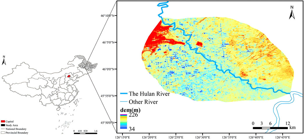
Figure 1. Overview of the maize planting area in the Hulan River Basin.

Based on the distinct characteristics of the wet season in the region, the Penman–Monteith formula (ElNesr and Alazba, 2012) was used to calculate the water demand of the main crops in the region, and the results were used for subsequent land use/cover planning in Equation 1:

${\text{ET}}_0=\frac{0.408∆\left({\mathrm{R}}_{\mathrm{n}}-\mathrm{G}\right)+\mathrm{\gamma }900{\mathrm{u}}_2\left({\mathrm{e}}_{\mathrm{s}}-{\mathrm{e}}_{\mathrm{a}}\right)/\left({\mathrm{T}}_{\text{mean}}+273\right)}{∆+\mathrm{\gamma }\left(1.034{\mathrm{u}}_2\right)},(1)$

where ET₀ is reference crop evapotranspiration, mm/d; R_n is net surface radiation, MJ/(m²·d); G is the soil heat flux MJ/(m²·d); T_mean is the daily average temperature, °C; U₂ is the wind speed at a height of 2 m, m/s; e_s is the saturated water pressure, kPa; e_a is the actual water pressure, kPa; Δ is the slope of the saturated water pressure curve, kPa/°C; and γ is the constant of hygrometer, kPa/°C.

According to the different stages of crop growth (initial, mid-growth, maturity, etc.), K_c for different growth periods was obtained by referring to the crop coefficient table provided by FAO, and the actual crop evapotranspiration (ET_c) was then calculated using Equation 2:

${\text{ET}}_{\mathrm{c}}={\text{ET}}_0\times {\mathrm{K}}_{\mathrm{c}},(2)$

where ET_c is actual crop evapotranspiration, mm/d.

The deduction of effective precipitation (P_e) was calculated using Equation 3:

${\mathrm{P}}_{\mathrm{e}}=\mathrm{P}\times \text{Utilisation\hspace{0.17em}factor},(3)$

where P is the total precipitation, mm. The utilization factor is determined by factors such as soil type and topography.

Based on P_e obtained from the abovementioned calculation, the irrigation water requirement (IWR) was calculated using Equation 4:

$\text{IWR}={\text{ET}}_{\mathrm{c}}-{\mathrm{P}}_{\mathrm{e}},(4)$

where the irrigation water requirement is recorded as 0 (no irrigation required) when P_e > ET_c.

2.2 Interpretation of land use

Landsat-TM remote sensing image data with cloud volume ≤5% from 2010 to 2020 were downloaded from the official website of NASA. The downloaded remote sensing image data were preprocessed by radiometric calibration, atmospheric correction, band synthesis, and image clipping. According to the classification system of the Chinese Academy of Sciences (CAS), land use was divided into farmland, forest, grassland, water, construction, unused land, and wetland (the first-level classification). Because of the different crop phenology information, the farmland in the Hulan River Basin was further divided into maize, soybean, rice, and other crops (the second-level classification). The spatial distribution maps of land use types were visualized using ArcGIS.

Due to the construction of a wetland park at the Hulan River Estuary in the Hulan River research area in 2018, there was a significant error in constructing the model using the 2020 land use/cover situation. Therefore, the actual model was constructed using the land use/cover change situation from 2010 to 2015, and the 2020 land use/cover situation was selected as the initial state for future simulation. Figure 2A shows the land use/cover situation under the first-level classification of the Hulan River research area in 2020, and Figure 2B shows the land use/cover situation under the second-level classification of the same area in 2020.

Figure 2

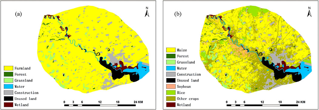
Figure 2. Land use/cover situation of the Hulan River research area in 2020. (A) The first-level classification, (B) The second-level classification.

2.3 CLUE-S model construction

The CLUE-S framework is designed to analyze transformations in land use and land cover within a defined geographical area. It integrates physical and environmental factors with socio-economic influences to provide a comprehensive understanding of the spatial and temporal dynamics of land use and land cover. Developed by a team of researchers from Wageningen University in the Netherlands, led by P.H. Verburg, the CLUE-S builds upon the foundational work of its predecessor, the CLUE model. The model posits that regional shifts in land use and land cover are propelled by the demand for these uses and covers, with their distribution in equilibrium with regional land demand, as well as the natural and socio-economic context. Utilizing systems theory, the CLUE-S model manages the competitive interactions between various types of land use and land cover, enabling the concurrent simulation of their changes. The theoretical underpinnings of the CLUE-S model encompass the interconnectivity, stratification, rivalry, and relative stability inherent in land use and land cover transitions.

2.3.1 Selection and testing of driving factors

The driving factor is an important part of the CLUE-S model. Selecting driving factors that are highly correlated with the research area for simulation can provide a more accurate analysis of land use change in the region. The research area for land use/cover simulation should have no less than seven driving factors, including two categories: natural driving factors and humanistic driving factors. The determination of seven driving factors in the Hulan River research area is shown in Table 1.

Table 1

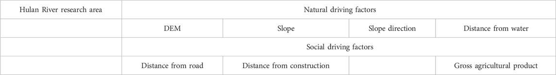
Table 1. Selection of driving factors for the research area.

The receiver operating characteristic (ROC) curves are instrumental in assessing the precision of selected drivers in simulating land use transitions within a study region. Figure 3 illustrates the ROC curves for various land uses in the Hulan River study area, with values spanning from 0.5 to 1, indicating their fitness for evaluation. A higher value signifies a greater capacity to explain the data. The figure reveals seven distinct land use/cover categories in the area, with water and construction land uses exhibiting perfect explanatory power, as indicated by an ROC value of 1. Wetlands have an ROC value of 0.94, indicating a strong explanatory capacity, while unused land and grasslands have values of 0.84 and 0.88, respectively, also demonstrating robust explanatory power. The ROC values for arable land and forests are comparatively lower, at 0.77 and 0.76, yet they still surpass the commonly accepted threshold of 0.75 for strong explanatory power. Consequently, a thorough analysis indicates that the model developed in this study possesses commendable explanatory capabilities.

Figure 3

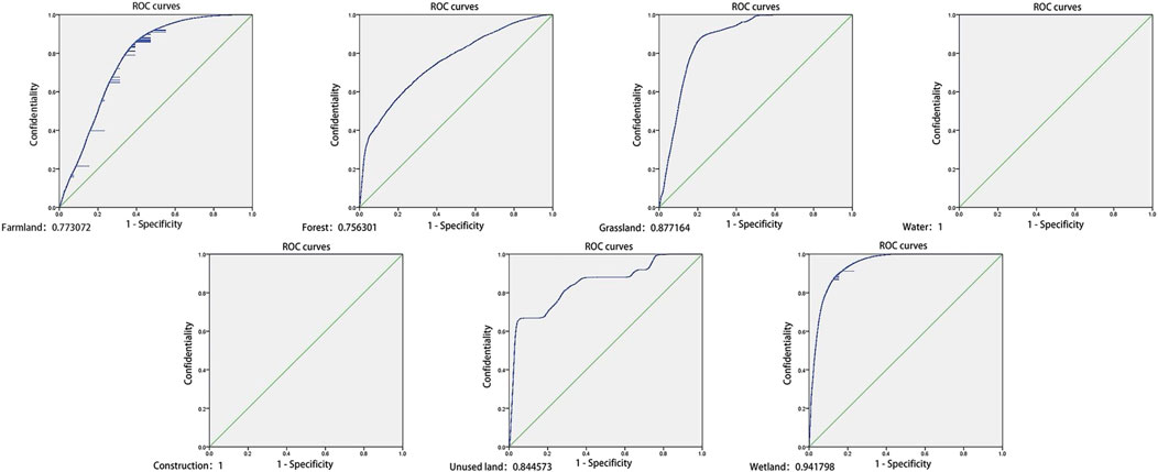
Figure 3. ROC curves of each land use type in the Hulan River research area.

2.3.2 Model file settings

The CLUE-S model includes a non-spatial analysis module and a space allocation module. The non-spatial analysis module is used to calculate the demand quantity of each category in the study area in the target year, which needs to be calculated by external models or mathematical methods. The spatial allocation module is based on the input of land demand parameters and the spatial distribution characteristics of driving factors and iteratively allocates the land category ownership of grid units, thereby achieving spatiotemporal simulations of land categories for each year. Table 2 shows all the space allocation module files required for the CLUE-S model.

Table 2

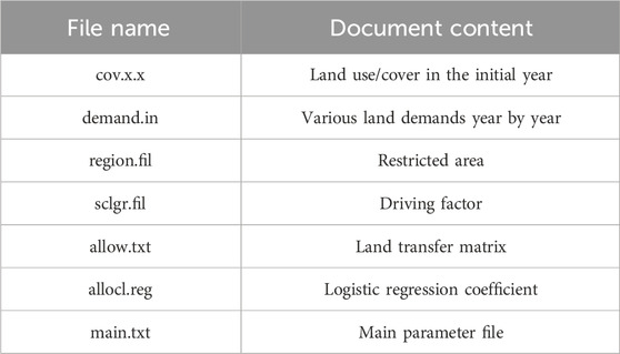
Table 2. Various documents required to build the CLUE-S model.

By comparing the land transfer situation in the Hulan River research area between 2010 and 2015, combined with other existing studies, the conversion elasticity of the Hulan River research area is set as shown in Table 3.

Table 3

Table 3. Conversion elasticity of land use/cover types.

2.4 Estimation of Net ecosystem productivity

Net ecosystem productivity (NEP) is the difference between the net primary productivity (NPP) of vegetation in an ecosystem and the fraction of photosynthetic products consumed by soil heterotrophic respiration (R_H), which was used as a measure of the carbon sink in Equation 5:

$\text{NEP}=\text{NPP}-{\mathrm{R}}_{\mathrm{H}}.(5)$

2.4.1 Estimation of NPP based on the CASA model

This study used ArcGIS 10.4 for data processing to estimate the NPP for the study area based on the CASA model. The CASA model is based on light energy utilization. It was developed by Potter et al. (1993). The model was subsequently refined by Potter and Klooster et al. It is applied in the studies of the carbon cycle and vegetation NPP (Potter et al., 1993).

NPP is calculated from the absorbed light and effective radiation available to the plant, along with the actual light utilization rate. The expression of NPP is shown in Equations 6–11:

$\mathrm{N}\text{PP}\left(\mathrm{x},\mathrm{t}\right)=\mathrm{A}\text{PAR}\left(\mathrm{x},\mathrm{t}\right)\times \mathrm{\epsilon }\left(\mathrm{x},\mathrm{t}\right),(6)$

where APAR(x, t) is the photosynthetic effective radiation absorbed by pixel x during month t (g C·m⁻²·month⁻¹) and ε(x, t) represents the actual light energy utilization by pixel x during month t (g C·m⁻²·month⁻¹).

$\text{APAR}\left(\mathrm{x},\mathrm{t}\right)=\text{SOL}\left(\mathrm{x},\mathrm{t}\right)\times \text{FPAR}\left(\mathrm{x},\mathrm{t}\right)\times 0.5,(7)$

$F\text{PAR}\left(\mathrm{x},\mathrm{t}\right)=\mathrm{\alpha }\text{FPA}{\mathrm{R}}_{\text{NDVI}}+\left(1-\mathrm{\alpha }\right)\text{FPA}{\mathrm{R}}_{\text{SR}},(8)$

$\text{FPA}{\mathrm{R}}_{\text{NDVI}}=\frac{\text{NDV}{\mathrm{I}}_{\left(\mathrm{x},\mathrm{t}\right)}-\text{NDV}{\mathrm{I}}_{\left(\mathrm{i},\min \right)}}{{\text{NDVI}}_{\left(\mathrm{i},\max \right)}-{\text{NDVI}}_{\left(\mathrm{i},\min \right)}}\times \left({\text{FPAR}}_{\max }-{\text{FPAR}}_{\min }\right)+{\text{FPAR}}_{\min },(9)$

$\text{FPA}{\mathrm{R}}_{\text{SR}}=\frac{{\text{SR}}_{\left(\mathrm{x},\mathrm{t}\right)}-{\text{SR}}_{\left(\mathrm{i},\min \right)}}{{\text{SR}}_{\left(\mathrm{i},\max \right)}-{\text{SR}}_{\left(\mathrm{i},\min \right)}}\times \left({\text{FPAR}}_{\max }-{\text{FPAR}}_{\min }\right)+{\text{FPAR}}_{\min },(10)$

$\text{SR}\left(\mathrm{x},\mathrm{t}\right)=\frac{1+\text{NDV}{\mathrm{I}}_{\left(\mathrm{x},\mathrm{t}\right)}}{1-\text{NDV}{\mathrm{I}}_{\left(\mathrm{x},\mathrm{t}\right)}},(11)$

where SOL(x, t) represents the total solar radiation of pixel x in month t (MJ C·m⁻²·month⁻¹); FPAR(x, t) represents the proportion of photosynthetically active radiation absorbed by the vegetation of pixel x in month t; the constant 0.5 indicates the proportion of the effective solar radiation (the wavelength is 0.38–0.71 μm) that the vegetation can use to the total solar radiation; NDVI (i, max) and NDVI (i, min) correspond to the maximum and minimum values of NDVI for vegetation type I, respectively, while SRmax and SRmin correspond to the percentage quantile at 5% and 95% of NDVI for vegetation type i, respectively. α is the adjustment factor for both methods of calculating FPAR, which is generally taken as 0.5. FPARmax is taken as 0.95, and FPARmin is taken as 0.001.

The expression of ε(x, t) is shown in Equations 12–15:

$\mathrm{\epsilon }\left(\mathrm{x},\mathrm{t}\right)={\mathrm{T}}_{{\mathrm{\epsilon }}_1}\left(\mathrm{x},\mathrm{t}\right)\times {\mathrm{T}}_{{\mathrm{\epsilon }}_2}\left(\mathrm{x},\mathrm{t}\right)\times {\mathrm{W}}_{\mathrm{\epsilon }}\left(\mathrm{x},\mathrm{t}\right)\times {\mathrm{\epsilon }}_{\max },(12)$

where T_ε1(x, t) and T_ε2(x, t) are the stress effects of low and high temperatures on light energy utilization, respectively; W_ε(x, t) refers to the water stress effect coefficient; and ε_max is the maximum light energy utilization of vegetation under ideal conditions.

T_ε1 is the reduction in vegetation first productivity due to the limitation of photosynthesis by the intrinsic biochemical action of the plant at low or high temperatures. It is calculated using Equation 13:

${\mathrm{T}}_{{\mathrm{\epsilon }}_1}\left(\mathrm{x},\mathrm{t}\right)=0.8+0.02\times {\mathrm{T}}_{\text{opt}}\left(\mathrm{x}\right)-0.0005\times {\left[{\mathrm{T}}_{\text{opt}}\left(\mathrm{x}\right)\right]}^2,(13)$

where T_opt(x) is the mean monthly temperature (°C) at which the vegetation NDVI value reaches its maximum.

T_ε2 represents the trend of gradually decreasing plant light energy utilization as the ambient temperature changes from T_opt(x) to high or low temperatures. It is calculated using Equation 14:

${\mathrm{T}}_{{\mathrm{\epsilon }}_2}=\frac{1.184}{1+\exp \left\{0.2\times \left[{\mathrm{T}}_{\text{opt}}\left(\mathrm{x}\right)-10-\mathrm{T}\left(\mathrm{x},\mathrm{t}\right)\right]\right\}}\times \frac{1}{\left.1+\{1+\exp [0.3\times (-{\mathrm{T}}_{\text{opt}}-10+\mathrm{T}\left(\mathrm{x},\mathrm{t}\right)]\right\}},(14)$

where T(x, t) is the average monthly temperature. When the average monthly temperature is 10°C higher or 13°C lower than the optimum temperature T_opt(x), the value of T_ε2 (x, t) for that month is equal to half the value of T_ε2(x, t) when the average monthly temperature T(x, t) was the optimum temperature T_opt(x). The expression of Wε(x, t) is shown in Equation 15:

${\mathrm{W}}_{\mathrm{\epsilon }}\left(\mathrm{x},\mathrm{t}\right)=0.5+0.5\times \mathrm{E}\left(\mathrm{x},\mathrm{t}\right)/{\mathrm{E}}_{\mathrm{p}}\left(\mathrm{x},\mathrm{t}\right),(15)$

where regional actual evapotranspiration E(x, t) is obtained according to the regional actual evapotranspiration model established by Zhou et al. (2002) and regional potential evapotranspiration E_p(x, t) is obtained according to the complementary relationship.

2.4.2 Estimation of R_H

R_H is calculated by referring to the empirical equation studied by Pei et al. (2009). It is calculated using Equation 16:

${\mathrm{R}}_{\mathrm{H}}=0.22\times \left[\exp \left(0.0912\mathrm{T}\right)+\ln \left(0.3145\mathrm{R}+1\right)\right]\times 30\times 46.5\%,(16)$

where R_H’s unit is g C·m⁻²·a⁻¹; T is the temperature (°C); and R is precipitation (mm).

2.5 Multi-objective linear programming

In addition to the spatial analysis module, other software applications or programs shall be used to complete the non-spatial analysis module. In this paper, the non-spatial analysis module used LINGO 18.0 for multi-objective linear programming (Yang et al., 2013). Interpreted data is used to create a land use transfer matrix for the study area. Considering local policies, agricultural water-saving, non-point source pollution control, and socio-economic benefits, equations are established from environmental and policy requirements; objective functions and constraint equations are established; and optimal land use/cover planning that meets all constraint conditions in the research area is analyzed.

Based on the carbon storage data of the study area obtained above, three assumptions are made for the possible future situation of the study area, namely, the priority scenario of grain crops (maximizing the planting area of grain crops), the priority scenario of ethanol fuel crops (maximizing the planting area of ethanol fuel crops), and the priority scenario of carbon storage (maximizing the total carbon storage of the research area).

According to the secondary land use/cover classification, all the land in the research area will be fully divided. The Hulan River research area included 10 categories, namely, maize, forest, grassland, water, construction, unused land, soybean, rice, other crops, and wetland. Among them, maize, soybean, rice, and other crops were integrated into the first-level classification of farmland. Table 4 shows the land use/cover equation codes and initial year (2020) allocation of the Hulan River research area.

Table 4

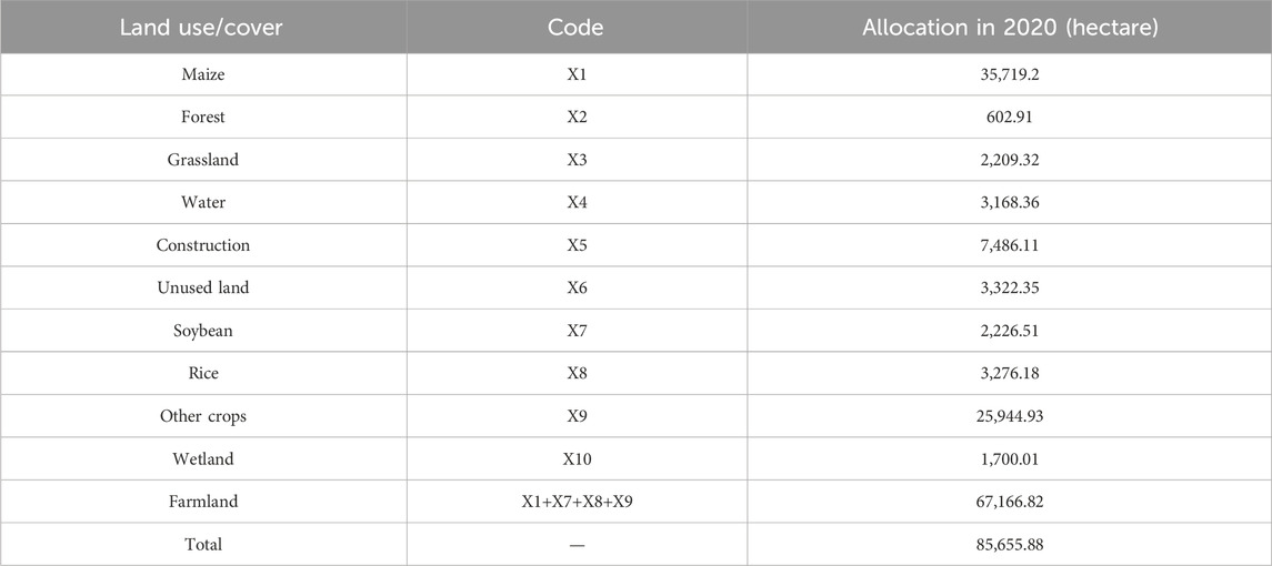
Table 4. Regression equation codes and initial year area of the research area.

The setting of constraint equations for the research area should include the following three aspects:

(1) Land area constraints

The total area of the study area should remain unchanged during the total research period.

$\mathrm{X}1+\mathrm{X}2+\mathrm{X}3+\mathrm{X}4+\mathrm{X}5+\mathrm{X}6+\mathrm{X}7+\mathrm{X}8+\mathrm{X}9+\mathrm{X}10=85655.88.$

(2) Indicator constraints

① Based on the purpose and practical requirements of minimizing pollutants, following a literature review and research by the same research group, it can be concluded that the main pollutants in farmland are total nitrogen and total phosphorus. Therefore, this paper integrates the existing research on soil nitrogen and phosphorus loads in the research area conducted by our research group and calculates the average nitrogen and phosphorus loads of soil under different land use/cover types. These values are used to represent the average nitrogen and phosphorus load caused by this type of land use/cover, with constraints aimed at minimizing nitrogen and phosphorus loads. Figure 4 shows the spatial distribution of nitrogen and phosphorus loads based on field studies and validated with published data.

Figure 4

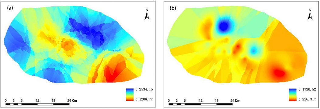
Figure 4. Nitrogen and phosphorus content of soil of the Hulan River Basin [(A) TN; (B) TP].

Total nitrogen minimization:

${\mathrm{MIN}}_{\text{TN}}=\mathrm{X}1*2035+\mathrm{X}7*1864+\mathrm{X}8*2027+\mathrm{X}9*1946.$

Total phosphorus minimization:

${\mathrm{MIN}}_{\text{TP}}=\mathrm{X}1*710+\mathrm{X}7*687+\mathrm{X}8*774+\mathrm{X}9*672.$

② To achieve the goal of minimizing water consumption, hypothesis constraints were applied to reduce water demand. This study utilizes the ET₀ calculator, a specialized program developed by the FAO (Food and Agriculture Organization of the United Nations). The software program integrates multiple calculation methods and is based on the Penman–Monteith equation, as mentioned in Equation (1). The irrigation water demand for the study area is determined by subtracting the effective precipitation, which is presented in Table 6 of Section 3.1.

MIN F(x) = ${\sum }_{\mathrm{x}=\mathrm{i}}^{\mathrm{t}}{\mathrm{b}}_{\mathrm{i}}{\mathrm{m}}_{\mathrm{i}}$, where b_i refers to the unit water consumption of the land use/cover type i and m_i refers to the area of the land use/cover type i.

${\mathrm{MIN}}_{\mathrm{W}}=\mathrm{X}1*252.95+\mathrm{X}7*121.90+\mathrm{X}8*201.512+\mathrm{X}9*192.92.$

③ To achieve the goal of maximizing economic benefits, the agricultural product wholesale website was consulted to obtain the purchase prices of the main agricultural products in the research area. Assuming the goal was to maximize economic benefits, an equation was constructed for this purpose. Economic benefits are embodied in the average purchase price of crops and total theoretical maximum output within a 1-year cycle (Table 5).

Table 5

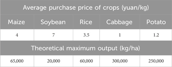
Table 5. Economic factors for the main crop types of the study area.

MAX F(x) = ${\sum }_{\mathrm{x}=\mathrm{i}}^{\mathrm{t}}{\mathrm{a}}_{\mathrm{i}}{\mathrm{m}}_{\mathrm{i}}$, where a_i refers to the output efficiency per unit area of the land use/cover type i and m_i refers to the area of the land use/cover type i.

${\mathrm{MAX}}_{\mathrm{Y}}=\mathrm{X}1*260000+\mathrm{X}7*140000+\mathrm{X}8*210000+\mathrm{X}9*300000.$

(3) Assumption scenario constraints

Under the three set scenario assumptions, constraints were established under different hypothetical conditions. The order of priority was to maximize the planting area of grain, fuel ethanol crops, and carbon sequestration.

① Maximizing the planting area of grain: ensuring the maximization of the planting area of grain crops (rice and maize).

${\mathrm{MAX}}_{\mathrm{R}}=\mathrm{X}1+\mathrm{X}8.$

② Maximizing the planting area of fuel ethanol crops: ensuring the maximization of the planting area of fuel ethanol crops (maize).

${\mathrm{MAX}}_{\mathrm{R}}=\mathrm{X}1.$

③ Maximizing carbon sequestration: ensuring the maximization of land use/cover types with significant carbon sequestration. The calculation process is detailed in Section 2.4 of this paper. The carbon sink results are shown in Table 7 of Section 3.3. The carbon sink capacity of each land use type is considered the key indicator for the equation as follows:

${\mathrm{MAX}}_{\mathrm{C}}=\mathrm{X}1*352.78+\mathrm{X}2*733.14+\mathrm{X}3*339.02+\mathrm{X}6*293.68+\mathrm{X}7*374.78+\mathrm{X}8*247.85+\mathrm{X}9*337.33.$

The overall technical route of the study is shown in Figure 5.

Figure 5

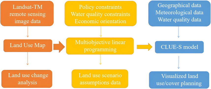
Figure 5. Technical route of the study.

3 Results and discussion

3.1 Water demand of the main crops

The ET₀ calculator, a specialized program developed by the Food and Agriculture Organization of the United Nations (FAO), is used to assist in the calculation of ET₀. The water demand calculation results are shown in Table 6. In the Hulan River Basin, there is no significant variation in the overall irrigation water demand. Notably, maize cultivation exhibits the highest irrigation water demand (252.77 mm) because of a higher K_c factor, while soybean cultivation has the lowest irrigation water demand (121.90 mm), representing a minimal difference of 130.87 mm between the two crops.

Table 6

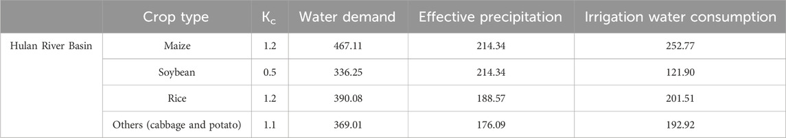
Table 6. Water demand data of different crops and irrigation water demand calculated using the Penman–Monteith formula in the study area (mm).

3.2 Land use interpretation results

The land use types of the Hulan River Basin included farmland, forest, grassland, water, construction, unused land, and wetland. Among them, the unused land was mainly swamp. According to the actual crop structures, farmland was subdivided into maize, rice, soybean, and other crops. The interpretation results of the three terms are displayed in Figure 6. The river channel at the outlet into the Songhua River was gentle and had abundant water. From 2010 to 2015, construction land was mostly distributed on the north bank. After 2015, the area of construction land increased across the river.

Figure 6

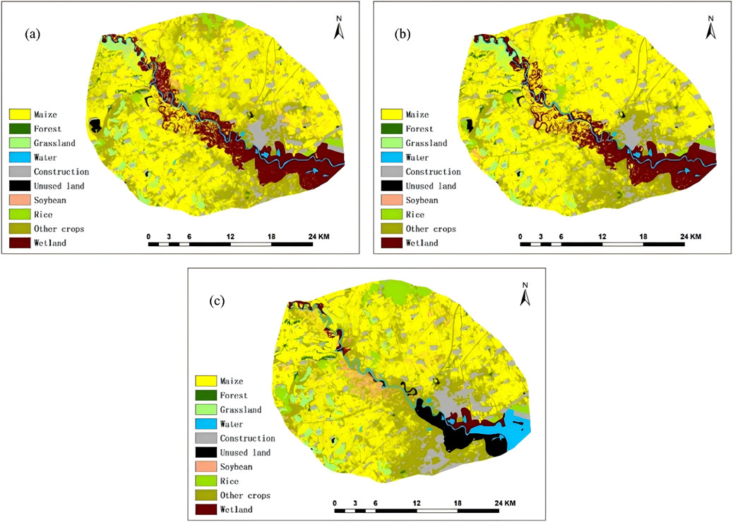
Figure 6. Land use/cover of the Hulan River Basin [(A) 2010; (B) 2015; and (C) 2020].

Figures 7, 8 depict the dynamics of land use transfers in the Hulan River Basin over 2010–2020. During the period of 2010–2015, the most prominent alteration in land use, in terms of area modification, was observed with the conversion of other cultivated land to maize cultivation. This transformation covered an extensive area of approximately 6704.46 ha, primarily concentrated in the northern and northwestern sectors of the study area. Furthermore, a significant land area of approximately 4644.27 ha underwent a transition from maize to other crops, with the main concentration observed in the southern and western sectors of the study area. Additionally, in the western part of the study area, an area of approximately 1392 ha, previously dominated by soybean, was predominantly converted to maize. Among the land use transfers involving forest, grassland, water, construction, and wetland, the transition toward maize exhibited the most pronounced spatial change. Consequently, there was a significant expansion in the extent of maize from 2010 to 2015. Notably, approximately 78% of the region remained unaffected by any alterations in land use types.

Figure 7

Figure 7. Chords of land use transfer in the Hulan River Basin [(A) 2010–2015 and (B) 2015–2020].

Figure 8

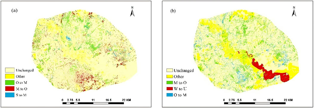
Figure 8. Spatial distribution of land use transfer in the Hulan River Basin [(A) 2010–2015 and (B) 2015–2020].

From 2015 to 2020, the most prominent land use change in the Hulan River Basin was the conversion of maize to other crops, encompassing approximately 9161.64 ha. It exhibited a wide distribution, albeit with relatively lower occurrences observed in the southeastern direction. The second noteworthy land use change involved the conversion of beach land to unused land, amounting to approximately 1953.36 ha, primarily concentrated near the riverbanks in midstream and downstream of the river. Additionally, there was a significant and widespread transformation of approximately 2918.61 ha of other crops into maize.

3.3 Distribution characteristics of carbon sink in the Hulan River basin

The Hulan River Basin’s carbon sink was estimated using the CASA model. According to the results, the carbon sink was estimated to be 329.35 gC·m⁻²·a⁻¹ in 2010, but it decreased to 295.59 gC·m⁻²·a⁻¹ in 2015. In 2020, 350.76 gC·m⁻²·a⁻¹ of the carbon sink was achieved. According to Zhou et al. (2023), which covered the Heilongjiang Province from 2010 to 2020, the average yearly NEP was 329.77 gC·m⁻²·a⁻¹. The NEP ranged from 281.38 gC·m⁻²·a⁻¹ to 380.07 gC·m⁻²·a⁻¹, suggesting a consistent trend with this paper. Specifically, between 2010 and 2015, NEP in the Hulan River Basin decreased by 33.96 gC·m⁻²·a⁻¹. However, from 2015 to 2020, NEP increased by 55.64 gC·m⁻²·a⁻¹. For each land use type, the carbon sink capacity is shown in Table 7.

Table 7

Table 7. Carbon sequestration of various land use types in the study area (g/m²).

Figure 9A illustrates the temporal distribution pattern of the Hulan River Basin’s NEP, with an initial increase followed by a decrease. In 2010, the highest NEP was observed in July, reaching 107.08 gC·m⁻²·a⁻¹. The NEP levels in January, February, and December were comparatively lower, ranging from roughly 0.5 to 0.6 gC·m⁻²·a⁻¹. The peak of NEP in 2015 was measured in August at 78.67 gC·m⁻²·a⁻¹, which was less than the maximum values documented for 2020 and 2010. In addition, there was a slight decrease in NEP in April, and the lowest monthly average value, 0.44 gC·m⁻²·a⁻¹, appeared in December. In 2020, the carbon sink in the Hulan River Basin exhibited its highest monthly average value in July, reaching 114.51 gC·m⁻²·a⁻¹. Conversely, the lowest monthly average value was observed in January, amounting to 0.35 gC·m⁻²·a⁻¹.

Figure 9

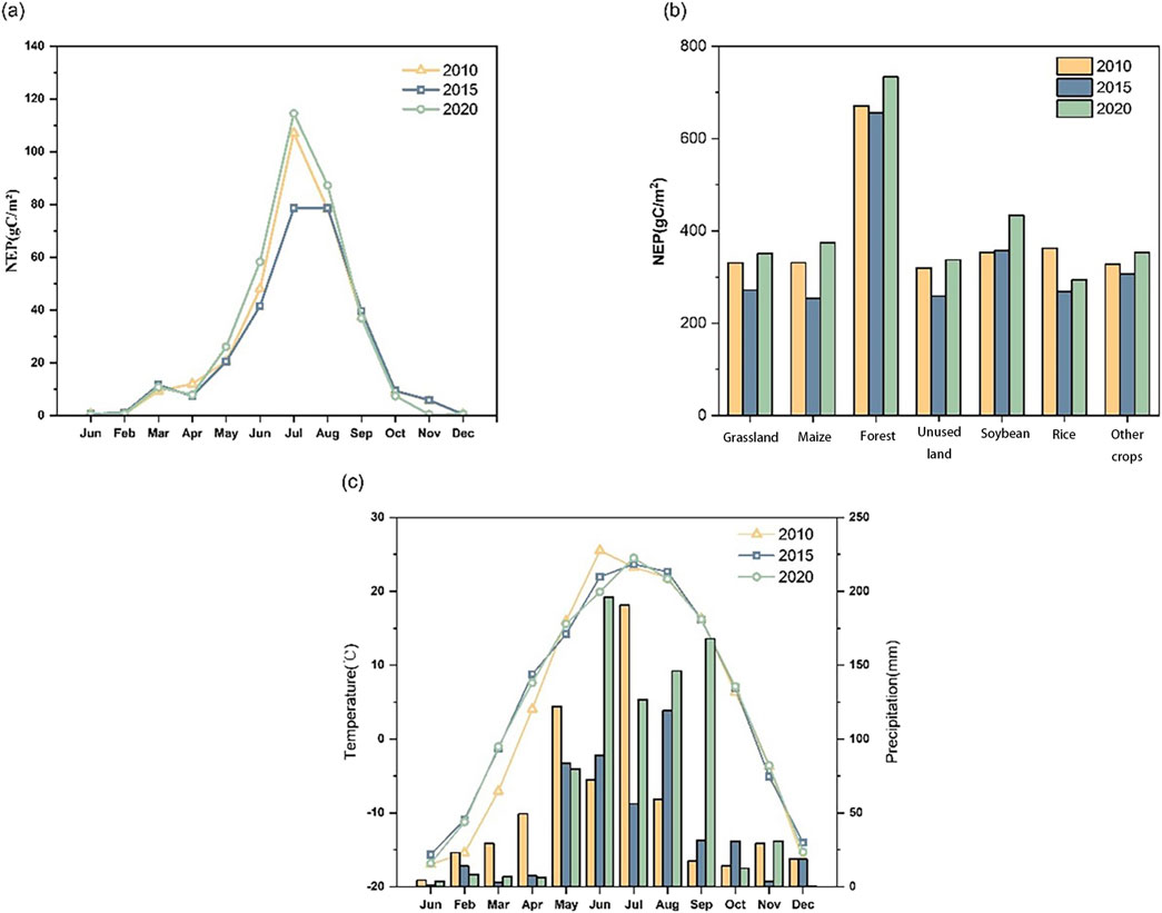
Figure 9. (A) Monthly average NEP of the Hulan River Basin. (B) NEP values for different land use types in the Hulan River Basin. (C) Monthly average temperature and precipitation of the Hulan River Basin.

According to Figure 9B, variations in land use types and their per unit area carbon sink capacities were observed in 2010, 2015, and 2020. Notably, forests showed higher NEP values due to their higher vegetation cover and carbon sequestration capabilities, while grassland and farmland showed varying performance. As the main crop in the area, soybean obtained relatively higher carbon sequestration than maize and rice. Noppol et al. (2022) found that the conversion of forest to agricultural land significantly reduced carbon stocks, while some conversions to grassland increased carbon stocks. Soil erodibility varied with the type of land use, with lower erodibility in grasslands due to higher organic carbon content and lower silt concentration. In contrast, chernozem soil, commonly found in Heilongjiang Province, typically has higher silt and clay concentrations, which benefits the fertile agricultural practices of maize and soybean cultivation. Therefore, unlike the grassland ecosystems of northern China (Li et al., 2023), policies aimed at returning forest or grassland grazing to grassland areas are not suitable for the Hulan River Basin.

Previous papers have indicated that climate change has certain influences on carbon sinks (Wang et al., 2021; Xu et al., 2023). Temperature and precipitation changes are factors directly influencing vegetation photosynthetic activity and soil respiration. Higher temperatures can enhance photosynthesis up to a threshold, while extreme precipitation variability may disrupt carbon sequestration (Wang et al., 2023; Arunrat et al., 2018). The stimulation of vegetation’s photosynthetic activity and subsequent vegetation growth are facilitated by the elevated temperatures (Yuan et al., 2023). Moderate precipitation plays a critical role in facilitating optimal vegetation growth. Inadequate or excessive rainfall can exert deleterious impacts on vegetation growth, thereby significantly influencing the magnitude of NEP (Li et al., 2021). The crucial developmental phase for vegetation, wherein it grows from initiation to maturity, typically occurs during June and July each year. NEP for all 3 years peaks between June and September, indicating that the carbon absorption capacity of ecosystems is the strongest in the warm seasons. After the peak, NEP rapidly decreases by November, showing a clear seasonal pattern. The seasonal variations in temperature and precipitation directly influence NEP, resulting in increased NEP during these months. In 2020, the Hulan River Basin experienced relatively high levels of temperature and precipitation from June to August, ensuring optimal water-thermal conditions for vegetation and effectively enhancing vegetation’s photosynthetic capacity. Consequently, land use types such as grassland and soybean exhibited the highest carbon sink per unit area among the 3 years. Conversely, lower precipitation levels were recorded from June to August 2015, contributing to regional aridity and restricted vegetation growth. Hence, grassland, soybean, and other land use types demonstrated the lowest carbon sink per unit area in that particular year.

The Hulan River Basin is in Heilongjiang Province, which is characterized by a cold temperate and temperate continental monsoon climate. Summers are hot, while winters are frigid and dry, with temperatures dropping below 0°C. There were discernible seasonal fluctuations in NEP. The carbon sink per unit area underwent a substantial increase during the months of April and May, whereas a rapid decrease was observed after July and August. Previous studies have provided substantial evidence to support the notion that precipitation exerts primary control over the NEP of China’s terrestrial systems (Zhang et al., 2023). Hence, the carbon sink per unit area in July 2015 exhibited a notable decrease compared to the peak values observed in July 2010 and 2020. In both 2015 and 2020, a discernible decrease in monthly NEP was observed. This decrease can be attributed to agricultural activities and the significant reduction in April precipitation levels, especially when compared to those of 2010. The observed decrease in monthly NEP during these periods can be attributed to unfavorable hydrothermal conditions.

The carbon sink classification in the Hulan River Basin used the natural breakpoint method, where the range of 0–253 gC·m⁻²·a⁻¹ was designated as the low carbon sink zone, 253–426 gC·m⁻²·a⁻¹ was designated as the medium carbon sink zone, and 426–1,075 gC·m⁻²·a⁻¹ was designated as the high carbon sink zone. As depicted in Figure 10, in 2010, the low carbon sink regions were predominantly located near the southeastern floodplains and riverbanks, with a substantial portion classified as medium carbon sink zones. Conversely, the high carbon sink regions are primarily concentrated in the northwestern area of the study area.

Figure 10

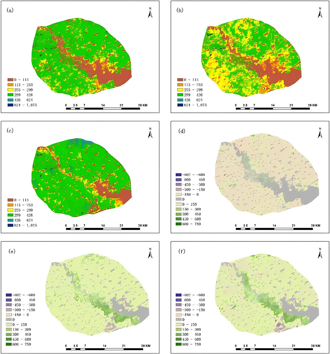
Figure 10. Spatial distribution of NEP (gC·m⁻²·a⁻¹) in the Hulan River Basin [(A) 2010; (B) 2015; and (C) 2020]. Spatial distribution of changes in NEP (gC·m⁻²·a⁻¹) in the Hulan River Basin [(D) 2010; (E) 2015; and (F) 2020].

From 2010 to 2015, there was a noticeable decrease in the carbon sink. The low carbon sink areas remained concentrated near the southeastern floodplains and riverbanks, while the medium carbon sink zones showed a more extensive distribution. Notably, the high carbon sink areas experienced a significant reduction in the northwestern part of the study area.

However, in 2020, there was a marked increase in carbon sink. The low carbon sink areas persisted near the southeastern floodplains, albeit with a diminished spatial extent. The medium carbon sink zones demonstrated a pronounced increase and wider distribution. The high carbon sink regions were concentrated in the northwestern and northern parts of the study area. Over the period from 2010 to 2020, the Hulan River Basin witnessed an overall increase in NEP. The northwest had a discernible decrease in NEP and an increase in carbon sinks close to the water.

3.4 Land use scenario assumptions in the Hulan River Basin

Table 8 shows the results of multiple linear regression in the research area. From the data, under the Grain Crop Priority Policy, the planting area of rice and maize has reached maximum, and the rice area has increased significantly compared to the other two assumptions and the situation in 2020. Under the Ethanol Crop Priority Policy, the priority of rice yield is reduced, and maize yield is further expanded to reach the maximum value among various assumed types. Under the carbon sequestration priority policy, the area of forest and grassland has been increased to the maximum of the three assumptions, resulting in the farmland area under this assumption reaching the minimum of the three assumptions. Under the three policies, the areas of other crops, unused land, and wetland have all decreased, indicating that these three types of land are relatively unimportant in policy planning.

Table 8

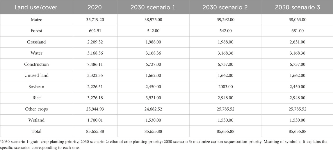
Table 8. Multiple linear regression results in the research area (hectare).

3.4.1 Grain Crop Priority Policy

Figure 11A shows the land use/cover situation under the Grain Crop Priority Policy in 2030, and Figure 11B shows the land use/cover change situation from 2020 to 2030. The specific area demand value can be found in Table 8. Under this policy, the area of maize, soybean, and rice has all increased. At the same time, while the total farmland area increased by 3255.8 ha, the area of other crops except for maize, soybeans, and rice decreased by 1262.41 ha, and other land use/cover types also had varying degrees of reduction. The area of unused land and wetland on the north bank of the estuary has decreased, while the grassland has increased, having been transferred from water and unused land. This reflects efforts to restore natural habitats or use previously undeveloped land. The transformation of unused land to grassland could indicate a positive trend toward land restoration or a strategy to prevent land degradation. However, the change in water area might raise environmental concerns due to the loss of biodiversity and natural water regulation provided by wetlands. In this situation, the area of maize and rice increases, with the main increase being in the unused land on the south bank of the estuary, while the rice area mainly increases near the existing rice planting area.

Figure 11

Figure 11. Simulation results under the Grain Crop Priority Policy in the research area. (A) 2030 (B) Change situation from 2020 to 2030.

3.4.2 Fuel Ethanol Crop Priority Policy

Figure 12A shows the land use/cover situation under the Fuel Ethanol Crop Priority Policy in 2030, and Figure 12B shows the land use/cover changes from 2020 to 2030. The specific area’s demand value can be found in Table 8. In this scenario, the area of maize as the only fuel ethanol crop in the research area has increased by 3572.8 ha, while all other land use/cover areas have decreased, with soybean, rice, and other crops decreasing by 223.51 ha, 328.18 ha, and 159.41 ha, respectively. Under the Fuel Ethanol Crop Priority Policy, the area of maize has significantly increased, like in scenario 1. The main growth point of maize is on the south bank of the estuary. At the same time, due to the reduction in soybean, rice, and other crops, a portion of the farmland near maize has also been converted to maize cultivation. The situation is similar to the Grain Crop Priority Policy, which shows the dual actions of maize in food security and fuel ethanol production promotion. This scenario illustrates a dynamic landscape where agricultural expansion, especially maize cultivation, is prominent, along with significant transitions from natural or unused lands to more productive uses.

Figure 12

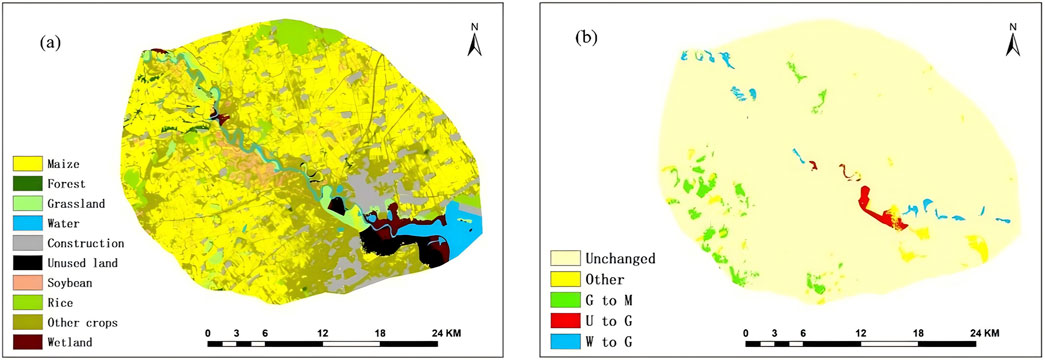
Figure 12. Simulation results under the Fuel Ethanol Crop Priority Policy in the research area. (A) 2030 (B) Change situation from 2020 to 2030.

3.4.3 Carbon Storage Priority Policy

Figure 13A shows the land use under the Carbon Storage Priority Policy in 2030, and Figure 13B shows the land use/cover change from 2020 to 2030. The specific area demand value can be found in Table 8. In this scenario, the area of forest and grassland, which have the largest carbon sink per unit area, increased by 61.09 ha and 221.68 ha, respectively, and the area of maize increased by 5.44%, with a total area of 1943.97 ha. The same trend appears in soybean cultivation. All other land use/cover areas decreased, including rice and other crops by 328.18 ha and 159.41 ha, respectively. Maize and soybean perform well in carbon storage, especially in Heilongjiang Province where a suitable planting environment is provided. The prominent constraint for maize expansion is the water pollution effect, which reminds the government to pay attention to non-point source pollution prevention while promoting maize planting. In the southern part of the area, construction land is transferred to maize, which may have benefits for water pollution control and carbon sink purposes. In this scenario, the forest area and grassland area have significantly increased, and the main growth point of grassland is still the unused land on the south bank of the estuary. It is speculated that due to the difficulty of converting to forest, the growth rate of grassland in this scenario is even higher than forest. Unused land is relatively easily transferred because of its high elasticity. It transforms grassland near the water body into a transition zone from water to wetland.

Figure 13

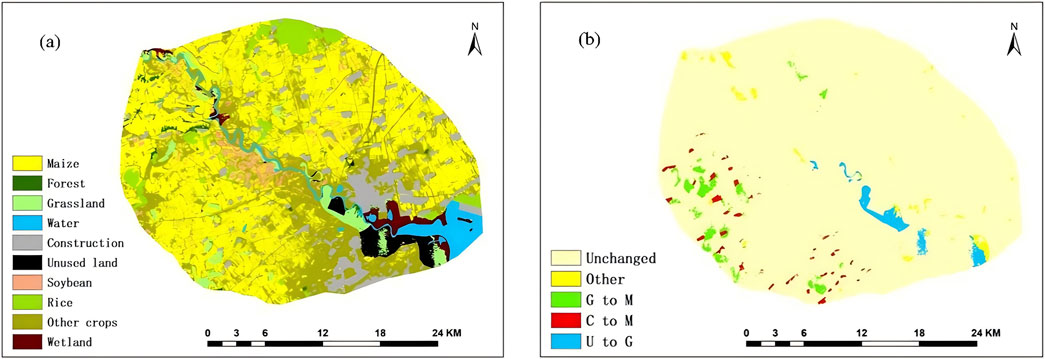
Figure 13. Simulation results under the Carbon Storage Priority Policy in the research area. (A) 2030 (B) Change situation from 2020 to 2030.

3.5 Carbon sinks of different scenario assumptions

The carbon sink status for three scenarios in 2030 was estimated by calculating the average NEP for each land use category based on the NEP values in 2020. The results are shown in Figure 14. Compared to 2020, scenario 1 shows a significant increase in the cultivated areas of maize and rice, with maize having a relatively high carbon sink per unit area. NEP has increased to approximately 4.67 × 10³ tC compared to 2020. In scenario 2, NEP has increased by 3.71 × 10³ tC compared to 2020. In scenario 3, the primary focus is on maintaining the carbon sink in the study area. Therefore, the forest and grassland areas with higher carbon sink potential have expanded. This has led to an overall improvement in the regional carbon sink capacity. Scenario 3 also has the highest NEP value among the three scenarios simulated. Compared to 2020, scenario 3 shows a substantial increase in the NEP value, with an addition of 8.32 × 10³ tC.

Figure 14

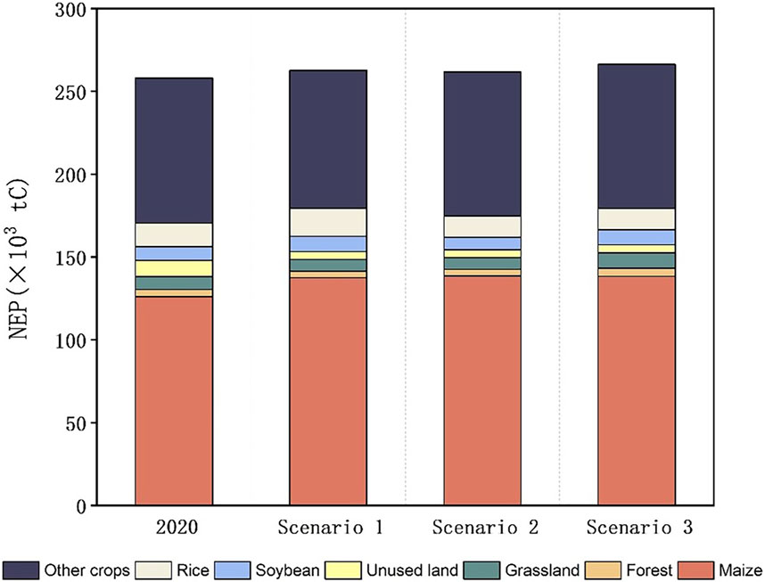
Figure 14. Various scenario simulations and 2020 NEP in the Hulan River Basin.

4 Conclusion

NEP in the Hulan River Basin follows a pattern of initial increase followed by a subsequent decrease over the annual cycle. Between 2010 and 2015, NEP decreased by 33.96 g of carbon per square meter per year, whereas from 2015 to 2020, an increase of 55.64 g of carbon per square meter per year was observed. The fluctuations in NEP are intricately linked to climatic conditions and land use practices within the Hulan River Basin. Spanning the decade from 2010 to 2020, areas with low carbon sequestration capabilities were predominantly found in the southeast of the region, showing a notable reduction in their geographic spread. Moderate carbon sink areas were more ubiquitous, with a lower frequency in the northwest. High carbon sink areas were largely situated in the northwest, forming the primary concentration of such zones.

The land demand is simulated within the study area under three distinct policy frameworks: the Grain Crop Priority Policy, the Fuel Ethanol Crop Priority Policy, and the Carbon Storage Priority Policy. This simulation was conducted to translate the developed CLUE-S model and ArcGIS outputs into a visual representation of future land use/cover. The results reveal that under scenario 1, which ensures regional food production, there is an expansion of arable land by 1262.41 ha. Scenario 2, prioritizing regional fuel ethanol output, observes an increase in the area dedicated to maize cultivation by approximately 3572.8 ha. Scenario 3, focused on bolstering the regional carbon sink, leads to substantial growth in both forested and grassland areas. Collectively, these three hypothetical scenarios within the study area effectively fulfill the preset requirements for the corresponding land use/cover categories.

The simulation of land use/cover in the research area in 2030 under four possible future scenarios was visualized based on the secondary classification. The conclusion proves that the land use/cover planning of typical fuel ethanol crop planting areas under different policy orientations can meet the needs of this policy, and its change pattern conforms to the literature description and actual situation, which has practical reference value.

In addition, the study assessed the carbon sequestration performance across a range of hypothetical scenarios, demonstrating a substantial increase in carbon capture for all scenarios compared to the baseline year of 2020. The outcomes highlight the substantial impact of each scenario in enhancing regional carbon sequestration potential, offering substantial empirical data and theoretical support for local policy formulation. Crucially, the study’s findings are of considerable importance for shaping future regional land use strategies and refining land use configurations.

Data availability statement

The raw data supporting the conclusions of this article will be made available by the authors, without undue reservation.

Author contributions

GC: writing–original draft, conceptualization, formal analysis, investigation, and methodology. HW: conceptualization, software, visualization, and writing–original draft. XL: data curation, visualization, and writing–original draft. WL: data curation, visualization, and writing–original draft. HL: funding acquisition and writing–review and editing. LD: project administration, supervision, writing–review and editing, and funding acquisition.

Funding

The author(s) declare that financial support was received for the research, authorship, and/or publication of this article. This research was financially supported by the National Natural Science Foundation of China (grant no. 41861124004) and the Social Science Project of Jilin Provincial Department of Education (grant no. JJKH20231248SK).

Conflict of interest

The authors declare that the research was conducted in the absence of any commercial or financial relationships that could be construed as a potential conflict of interest.

Generative AI statement

The author(s) declare that no Generative AI was used in the creation of this manuscript.

Publisher’s note

All claims expressed in this article are solely those of the authors and do not necessarily represent those of their affiliated organizations, or those of the publisher, the editors and the reviewers. Any product that may be evaluated in this article, or claim that may be made by its manufacturer, is not guaranteed or endorsed by the publisher.

Abbreviations

NEP, net ecosystem productivity; ET, evapotranspiration; TN, total nitrogen; TP, total phosphorus; ROC, receiver operating characteristic; NPP, net primary productivity; RH, fraction of photosynthetic products consumed by soil heterotrophic respiration.

References

Ahmed, N., Wang, G. X., Booij, M. J., Marhaento, H., Pordhan, F. A., Ali, S., et al. (2022). Variations in hydrological variables using distributed hydrological model in permafrost environment. Ecol. Indic. 145, 109609. doi:10.1016/j.ecolind.2022.109609

CrossRef Full Text | Google Scholar

Arunrata, N., Piumijumnong, N., and Hatano, R. (2018). Predicting local-scale impact of climate change on rice yield and soil organic carbon sequestration: a case study in Roi Et Province, Northeast Thailand. Agric. Syst. 164, 58–70. doi:10.1016/j.agsy.2018.04.001

CrossRef Full Text | Google Scholar

Chen, L. D., and Fu, B. J. (2000). Farmland ecosystem management and control of non Point source pollution. Environ. Sci. 21 (02), 98–100. doi:10.13227/j.hjkx.2000.02.025

CrossRef Full Text | Google Scholar

ElNesr, M. N., and Alazba, A. A. (2012). Simple statistical equivalents of Penman–Monteith formula’s parameters in the absence of non-basic climatic factors. Arabian J. Geosciences 5 (4), 757–767. doi:10.1007/s12517-010-0231-1

CrossRef Full Text | Google Scholar

Hassan, D. F., Abdalkadhum, A. J., Mohammed, R. J., and Shaban, A. (2022). Integration remote sensing and meteorological data to monitoring plant phenology and estimation crop coefficient and evapotranspiration. J. Ecol. Eng. 23 (4), 325–335. doi:10.12911/22998993/146267

CrossRef Full Text | Google Scholar

He, Y., Yang, A. J., Chen, W. J., Guo, Y., Feng, Y. H., and Song, X. (2022). Agricultural non Point source pollution load and distribution characteristics of typical watershed in southwest Karst Plateau mountain area. Res. Soil Water Conservation 29 (01), 148–152. doi:10.13869/j.cnki.rswc.20210803.001

CrossRef Full Text | Google Scholar

Li, H. Z., and Zhang, M. X. (2019). A review on the calculation of non-point source pollution loads. IOP Conf. Ser. Earth Environ. Sci. 344 (1), 012138. doi:10.1088/1755-1315/344/1/012138

CrossRef Full Text | Google Scholar

Li, J. S., Guo, X. M., Chuai, X. W., Xie, F. J., Yang, F., Gao, R. Y., et al. (2021). Reexamine China’s terrestrial ecosystem carbon balance under land use-type and climate change. Land Use Policy 102, 105275. doi:10.1016/j.landusepol.2020.105275

CrossRef Full Text | Google Scholar

Li, W. B., Liang, Y. J., Liu, L. J., He, Q. Q., Huang, J. J., and Yin, Z. C. (2024). Spatio-temporal impacts of land use change on water-energy-food nexus carbon emissions in China, 2011-2020. Environ. Impact Assess. Rev. 105, 107436. doi:10.1016/j.eiar.2024.107436

CrossRef Full Text | Google Scholar

Li, Z. W., Tang, Q., Wang, X., Chen, B. R., Sun, C. M., and Xin, X. P. (2023). Grassland carbon change in northern China under historical and future land use and land cover change. Agronomy 13 (8), 2180. doi:10.3390/agronomy13082180

CrossRef Full Text | Google Scholar

Liang, Y. J., Liu, L. J., and Huang, J. J. (2017). Integrating the SD-CLUE-S and InVEST models into assessment of oasis carbon storage in northwestern China. PLOS ONE 12 (2), e0172494. doi:10.1371/journal.pone.0172494

PubMed Abstract | CrossRef Full Text | Google Scholar

Liu, M., Li, C. L., Hu, Y. M., Sun, F. Y., Xu, Y. Y., and Chen, T. (2014). Combining CLUE-S and SWAT models to forecast land use change and non-point source pollution impact at a watershed scale in Liaoning Province, China. Chin. Geogr. Sci. 24 (5), 540–550. doi:10.1007/s11769-014-0661-x

CrossRef Full Text | Google Scholar

Liu, Y. G., and Wang, L. Y. (2021). Research on simulation and prediction of land use change in Jinan City. Territ. and Nat. Resour. Study 190 (01), 47–50. doi:10.16202/j.cnki.tnrs.2021.01.013

CrossRef Full Text | Google Scholar

Mao, K. Y., Fan, Y. L., Wang, Y., and Wang, Z. H. (2018). Current situation and deep analysis of fuel ethanol industry at home and abroad. High-Technology and Commer. 265 (06), 6–13.

Google Scholar

Ndegwa Mundia, C., and Murayama, Y. (2009). Analysis of land use/cover changes and animal population dynamics in a wildlife sanctuary in East Africa. Remote Sens. 1 (4), 952–970. doi:10.3390/rs1040952

CrossRef Full Text | Google Scholar

Noppol, A., Sukanya, S., Praeploy, K., and Ryusuke, H. (2022). Soil organic carbon and soil erodibility response to various land-use changes in northern Thailand. Catena 219, 106595. doi:10.1016/j.catena.2022.106595

CrossRef Full Text | Google Scholar

Pei, Z. Y., Ouyang, H., Zhou, C. P., and Xu, X. L. (2009). Carbon balance in an alpine steppe in the qinghai-tibet plateau. J. Integr. Plant Biol. 51 (5), 521–526. doi:10.1111/j.1744-7909.2009.00813.x

PubMed Abstract | CrossRef Full Text | Google Scholar

Peng, K. F., Jiang, W. G., Deng, Y., Liu, Y. H., Wu, Z. F., and Chen, Z. (2020). Simulating wetland changes under different scenarios based on integrating the random forest and CLUE-S models: a case study of Wuhan Urban Agglomeration. Ecol. Indic. 117, 106671. doi:10.1016/j.ecolind.2020.106671

CrossRef Full Text | Google Scholar

Potter, C. S., Randerson, J. T., Field, C. B., Matson, P. A., Klooster, S. A., Mooney, H. A., et al. (1993). Terrestrial ecosystem production: a process model based on global satellite and surface data. Glob. Biogeochem. Cycles 7 (4), 811–841. doi:10.1029/93GB02725

CrossRef Full Text | Google Scholar

Schmidt, N., and Zinkernagel, J. (2017). Model and growth stage based variability of the irrigation demand of onion crops with predicted climate change. Water 9 (9), 693. doi:10.3390/w9090693

CrossRef Full Text | Google Scholar

Su, Y. X., Liu, Y. H., Huo, L. J., and Yang, G. Q. (2024). Research on optimal allocation of soil and water resources based on water-energy-food-carbon nexus. J. Clean. Prod. 450, 141869. doi:10.1016/j.jclepro.2024.141869

CrossRef Full Text | Google Scholar

Wang, H. J., Cao, L., and Feng, R. (2021). Hydrological similarity-based parameter regionalization under different climate and underlying surfaces in ungauged basins. Water 13 (18), 2508. doi:10.3390/w13182508

CrossRef Full Text | Google Scholar

Wang, H. L., He, P., Shen, C., and Y. Wu, Z. (2019). Effect of irrigation amount and fertilization on agriculture non-point source pollution in the paddy field. Environ. Sci. Pollut. Res. 26 (10), 10363–10373. doi:10.1007/s11356-019-04375-z

PubMed Abstract | CrossRef Full Text | Google Scholar

Wang, M. M., Zhao, J., Wang, S. Q., Chen, B., and Li, Z. P. (2021). Detection and attribution of positive net ecosystem productivity extremes in China’s terrestrial ecosystems during 2000-2016. Ecol. Indic. 132, 108323. doi:10.1016/j.ecolind.2021.108323

CrossRef Full Text | Google Scholar

Wang, X., Wang, K., Zhang, Y., Gao, J., and Xiong, Y. (2023). Impact of climate on the carbon sink capacity of ecological spaces: a case study from the Beijing–Tianjin–Hebei urban agglomeration. Land 12 (8), 1619. doi:10.3390/land12081619

CrossRef Full Text | Google Scholar

Wei, X. G., Wang, T. L., Li, B., Liu, S. Y., Yao, M. Z., Xie, Y., et al. (2018). Study on the spatiotemporal distribution characteristics of water profit and loss in maize fields and irrigation model zoning in Liaoning Province. Trans. Chin. Soc. Agric. Eng. 34 (23), 119–126. doi:10.11975/j.issn.1002-6819.2018.23.014

CrossRef Full Text | Google Scholar

Wu, D., Zhang, Z. W., Liu, D., Zhang, L. L., Li, M., Khan, M. I., et al. (2024). Calculation and analysis of agricultural carbon emission efficiency considering water-energy-food pressure: modeling and application. Sci. Total Environ. 907, 167819. doi:10.1016/j.scitotenv.2023.167819

PubMed Abstract | CrossRef Full Text | Google Scholar

Wu, H., Yue, Q., Guo, P., and Xu, X. Y. (2025). Exploiting the potential of carbon emission reduction in cropping-livestock systems: managing water-energy-food nexus for sustainable development. Appl. Energy 377 (B), 124443. doi:10.1016/j.apenergy.2024.124443

CrossRef Full Text | Google Scholar

Xu, B. W., Niu, Y. R., Zhang, Y. N., Chen, Z. F., and Zhang, L. (2022). China’s agricultural non-point source pollution and green growth: interaction and spatial spillover. Environ. Sci. Pollut. Res. 29 (40), 60278–60288. doi:10.1007/s11356-022-20128-x

PubMed Abstract | CrossRef Full Text | Google Scholar

Xu, X., Liu, J., Jiao, F. S., Zhang, K. S., Ye, X., Gong, H. B., et al. (2023). Ecological engineering induced carbon sinks shifting from decreasing to increasing during 1981–2019 in China. Sci. Total Environ. 864, 161037. doi:10.1016/j.scitotenv.2022.161037

PubMed Abstract | CrossRef Full Text | Google Scholar

Yang, H. Q., Zhang, J., and Yang, Z. G. (2013). Rational land planning utilization structure optimization based on multi-objective linear programming model of foshan. Adv. Mater. Res. 616–618, 1243–1248. doi:10.4028/www.scientific.net/AMR.616-618.1243

PubMed Abstract | CrossRef Full Text | Google Scholar

Yuan, Z., Jiang, Q. Q., and Yin, J. (2023). Impact of climate change and land use change on ecosystem net primary productivity in the Yangtze River and Yellow River Source Region, China. Watershed Ecol. Environ. 5, 125–133. doi:10.1016/j.wsee.2023.04.001

CrossRef Full Text | Google Scholar

Yue, Q., Zhang, F., and Guo, P. (2018). Optimization-based agricultural water-saving potential analysis in minqin county, gansu province China. Water 10 (9), 1125. doi:10.3390/w10091125

CrossRef Full Text | Google Scholar

Zhang, C. L., Huang, N., Wang, L., Song, W. J., Zhang, Y. L., and Niu, Z. (2023). Spatial and temporal pattern of net ecosystem productivity in China and its response to climate change in the past 40 years. Int. J. Environ. Res. Public Health 20 (1), 92. doi:10.3390/ijerph20010092

PubMed Abstract | CrossRef Full Text | Google Scholar

Zhang, P., Liu, Y. H., Pan, Y., and Yu, Z. R. (2013). Land use pattern optimization based on CLUE-S and SWAT models for agricultural non-point source pollution control. Math. Comput. Model. 58 (3), 588–595. doi:10.1016/j.mcm.2011.10.061

CrossRef Full Text | Google Scholar

Zhao, M. M., He, Z. B., Du, J., Chen, L. F., Lin, P. F., and Fang, S. (2019). Assessing the effects of ecological engineering on carbon storage by linking the CA-Markov and InVEST models. Ecol. Indic. 98, 29–38. doi:10.1016/j.ecolind.2018.10.052

CrossRef Full Text | Google Scholar

Zhao, X., Tang, F., Zhang, P. T., Hu, B. Y., and Xu, L. (2019). Dynamic simulation and characteristic analysis of county production life ecological space conflict based on CLUE-S model. Acta Ecol. Sin. 39 (16), 5897–5908. doi:10.5846/stxb201901070059

CrossRef Full Text | Google Scholar

Zhou, F. C., Han, X. Z., Tang, S. H., Song, X. N., and Wang, H. (2021). An improved model for evaluating ecosystem service values using land use/cover and vegetation parameters. J. Meteorological Res. 35 (1), 148–156. doi:10.1007/s13351-021-9199-x

CrossRef Full Text | Google Scholar

Zhou, G. S., Wang, Y. H., Jiang, Y. L., and Yang, Z. Y. (2002). Estimating biomass and net primary production from forest inventory data: a case study of China’s Larix forests. For. Ecol. Manag. 169 (1), 149–157. doi:10.1016/S0378-1127(02)00305-5

CrossRef Full Text | Google Scholar

Zhou, S. H., Cao, J. Q., Wang, F., and Chang, Z. D. (2023). Spatio-temporal distribution and influencing factors of carbon source/sink, carbon surplus and deficit in three northeast provinces. Acta Ecol. Sin. 43 (22), 9266–9280. doi:10.20103/j.stxb.202212153598

CrossRef Full Text | Google Scholar