Analyzing the impact of economic growth and FDI on sustainable development goals in China: insights from ecological footprints and load capacity factors

This study investigates the impact of economic growth and foreign direct investment (FDI) on China’s sustainable development goals (SDGs), specifically Zero Hunger (SDG 2), Life Below Water (SDG 14), and Life on Land (SDG 15). It examines ecological footprints and load capacity factors (LCFs) in cropland, fishing, forest, and grazing land using Fourier bootstrap autoregressive distributed lag (ARDL) cointegration analysis and fully modified ordinary least squares (FMOLS) estimators. The study covers the period from 1979 to 2022. Key findings reveal that while GDP and FDI often exacerbate environmental degradation, urbanization and value-added agriculture, forestry, and fishing (FAFGDP) improve sustainability in some areas. The study confirms the pollution haven hypothesis for most models, suggesting that China’s legal and regulatory frameworks may inadequately mitigate FDI’s adverse environmental effects. The Environmental Kuznets Curve (EKC) hypothesis is not supported as GDP growth generally increases ecological footprints. However, trade openness and urbanization show positive influences on environmental sustainability. Policy recommendations include enhancing energy efficiency, promoting renewable energy, implementing green technologies in agriculture and urban development, and revising FDI policies to incentivize environmentally friendly practices. These strategies are crucial for achieving China’s sustainable development goals and mitigating the pressures of human activities on natural resources.

Introduction

Sustainable development is a growth model that satisfies current needs without compromising the ability of future generations to meet theirs. This approach aims to balance economic growth, social equity, and environmental sustainability. The United Nations’ 17 Sustainable Development Goals (SDGs) target eliminating poverty, protecting the planet, and ensuring peace and prosperity for all by 2030 (Sugiawan et al., 2023). The following variables are vital for measuring the sustainable management and use of natural resources.

The cropland footprint indicates the use of agricultural land for food production, highlighting the need for efficient and sustainable land use to ensure food security and ecosystem health. The cropland load capacity factor measures the pressure agricultural lands can sustainably bear, influencing food production sustainability. Similarly, the fishing grounds footprint (FGF) tracks the use of fishing areas for seafood, emphasizing the importance of sustainable practices to prevent overfishing and marine resource depletion. The fishing load capacity factor assesses the sustainable capacity of fishing grounds, determining the level of fishing activity that ecosystems can sustainably support.

The forest product footprint measures the consumption of forest products like timber and paper, underlining the need for sustainable forest management to conserve biodiversity and combat climate change. The forest load capacity factor evaluates how much resource extraction forests can sustainably support. The grazing land footprint represents the use of grazing areas for livestock, indicating the land required for meat and dairy production, and stresses the importance of sustainable grazing to prevent soil erosion and biodiversity loss. The grazing load capacity factor measures the sustainable utilization capacity of grazing lands, determining the sustainable level of livestock activity. These variables, known as sustainable development indicators, are essential for achieving sustainable development goals. Effective and sustainable resource management is crucial for preserving our capacity to meet the needs of future generations (Klimovskikh et al., 2023; Ulussever et al., 2024). Each indicator helps develop and implement strategies for sustainable resource use and management.

Several economic, social, and environmental factors influence sustainable development indicators. These include GDP, foreign trade openness, urbanization, agriculture, forestry, fishing value-added (AGR), and foreign direct investment (FDI). GDP can impact sustainable development indicators by improving agricultural technologies and practices, enhancing fishing technologies, and promoting the sustainable use of forest and livestock resources (Yang and Solangi, 2024). Foreign trade openness (OPN) can increase the demand for natural resources in international markets, potentially complicating their sustainable management. However, it also offers opportunities to import and adopt sustainable practices and technologies (Hasan and Du, 2023). Higher urbanization (URB) can convert agricultural and forest lands into urban areas, affecting their use and sustainability while increasing the demand for seafood, thereby putting pressure on fishing grounds (Bhattarai and Adhikari, 2023). Conversely, urban expansion can reduce the extent of grazing areas. Agriculture, forestry, and fishing value-added (AGR) can promote efficient and sustainable resource use, encouraging better management practices and technological innovations. FDI can provide the necessary financing and technology for sustainable resource management, although it can also lead to overuse and environmental degradation in some cases (Renyong and Sedik, 2023).

Therefore, GDP and FDI can facilitate the adoption of sustainable practices in agriculture, forestry, and fishing. OPN can increase natural resource demand while promoting sustainable technologies and practices. Higher URB can impact natural resource use and sustainability, often reducing agricultural and forest lands. Figure 1 illustrates the proportion of the Chinese population within the global population in 2023.

Figure 1

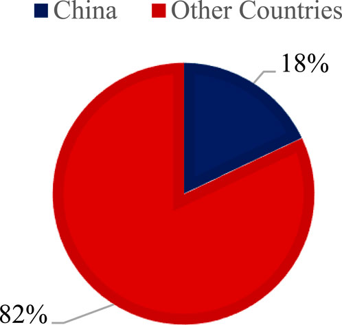
Figure 1. Population of China (2023) (World Bank, 2024a).

In 1961, the Chinese economy made up roughly 1.01% of the global GDP, but by 2023, this share had increased to 18.5% (World Bank, 2024a). Additionally, as depicted in Figure 1, China, with its swiftly growing economy and a population of 1.410 billion in 2023, comprises approximately 18% of the global population. This substantial GDP and population underscore the importance of sustainable natural resource management. Sustainable development is vital for sustaining China’s long-term economic growth, preventing environmental degradation, and ensuring social equity. Advancements in sustainable development goals will yield numerous benefits for the Chinese economy. For instance, efficient and sustainable agricultural land use will enhance food security, reduce import reliance, and boost agricultural production. Given China’s responsibility to feed a significant portion of the world’s population, progress in this area is crucial. Enhancing the sustainable use capacity of agricultural land is essential for maintaining soil fertility and ensuring ongoing agricultural production, thereby providing stability in the agricultural sector and supporting rural economic development.

Decreasing per capita use of fishing grounds will aid in protecting marine ecosystems and promoting sustainable fishing practices, ensuring the sustainable use of marine resources and bolstering economic sustainability in the fishing sector (Kemp et al., 2023). Increasing the sustainable use capacity of fishing grounds will prevent overfishing, protect marine ecosystems, ensure the sustainability of seafood production, and safeguard the livelihoods of local communities (Soeparna and Taofiqurohman, 2024). Reducing per capita use of forest products will foster forest conservation and sustainable forest management, helping preserve biodiversity and combat climate change (Rosenfeld et al., 2024). Enhancing the sustainable use capacity of forest ecosystems will protect their ecological functions and ensure the continued sustainable production of forest products, providing economic sustainability in the forest product sector and supporting rural livelihoods (Tampekis et al., 2024). Decreasing per capita use of grazing lands will prevent pasture overuse and maintain soil fertility, enhancing sustainability in the livestock sector and ensuring food security (Caradus et al., 2024). Increasing the sustainable use capacity of grazing lands will mitigate the negative impacts of livestock activities on ecosystems and maintain the long-term productivity of pastures, supporting economic sustainability in the livestock sector and strengthening rural economies (Li et al., 2024).

Therefore, the sustainable use of natural resources prevents environmental degradation and ecosystem destruction, playing a critical role in preserving biodiversity and combating climate change. Sustainable agricultural, forestry, and fishing practices support long-term economic growth and stability by promoting efficient resource use and building resilience against economic crises. Adopting sustainable practices in the agriculture and livestock sectors helps increase food production and security, essential for feeding China’s growing population. Sustainable development enhances economic opportunities in rural areas, protects local communities’ livelihoods, reduces income inequality between rural and urban areas, and ensures social equity. Achieving sustainable development goals will bolster China’s environmental leadership on the global stage and contribute to worldwide sustainability efforts.

Improvements in China’s sustainable development indicators will support long-term economic growth, ensure environmental protection, enhance social equity, and significantly contribute to global sustainability efforts. Consequently, the efficient and sustainable management of natural resources is crucial for China to achieve its sustainable development goals. The following information illustrates the proportions of the Chinese economy in global meat, milk, and egg production in 2021.

As shown in Figure 2, China accounted for 14% of global meat production in 2021 and approximately 37% and 5% of global egg and milk production, respectively. This substantial share in global production underscores the importance of sustainable natural resource management in China. Sustainable development indicators are crucial for strategic decision-making to ensure agriculture, livestock, and fishing sustainability (Yang and Solangi, 2024). For example, producing feed crops for meat and milk requires extensive agricultural land. The per capita agricultural land footprint is vital for efficient resource use.

Figure 2

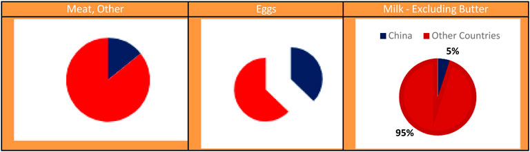
Figure 2. Meat, egg, and milk production in China (2021) (Food and Agriculture Organization of the United Nations, 2024).

Efficient agricultural land use ensures sustainable feed crop production, meeting the livestock sector’s needs and supporting meat and milk production sustainability.

Optimizing the feed crop production capacity guarantees the livestock sector’s continuity. Enhancing the agricultural lands’ load capacity ensures sustained and efficient feed production, stabilizing meat and milk production.

Fish and seafood production plays a crucial role, particularly for fish feed. The per capita fishing grounds footprint measures the efficiency of resource use. Sustainable fishing practices protect fish and seafood stocks, supporting fish feed production and enhancing feed resource sustainability in the livestock sector. Protecting fish stocks for fish feed production is critical, and optimizing the fishing load capacity ensures the protection and sustainability of fish stocks for fish feed production (Naghdi et al., 2024).

Forest products, such as feed additives and agricultural equipment, are used in various ways in the agriculture and livestock sectors. The sustainable use of forest products meets these sectors’ needs and supports their sustainability. Sustainable forest ecosystem use ensures biodiversity protection and indirectly supports agricultural and livestock activities. Increasing forest load capacity ensures forest resource protection and sustainable use, indirectly supporting the agriculture and livestock sectors.

Grazing lands are fundamental for meat and milk production in the livestock sector. The per capita grazing land footprint ensures efficient land use. Efficient grazing land use supports livestock sector sustainability and increases the animal product (meat and milk) production capacity. Optimizing environmental sustainability in livestock activities is necessary. Increasing the load capacity of grazing lands reduces the negative impacts of livestock activities on ecosystems and supports sustainable livestock production (Henn et al., 2024).

Therefore, China’s significant share in global meat, milk, and egg production necessitates the efficient and sustainable use of natural resources. Sustainable development ensures food security, environmental protection, economic sustainability, and long-term planning.

Conversely, economic sustainability and strategic long-term planning in agricultural production are vital for sustainable development. Figure 3 depicts the agricultural output of the top 10 economies with the highest global agricultural production in 2020.

Figure 3

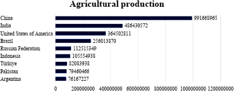
Figure 3. Agricultural production (2022) (Food and Agriculture Organization of the United Nations, 2024).

China’s status as the world’s second-largest producer of softwood and hardwood (including bamboo) (Statista, 2024; Wang et al., 2023), along with its leading role in agricultural production, as depicted in Figure 3, highlights the critical need for sustainable development indicators to sustainably manage and use natural resources. Key variables such as cropland footprint per capita, cropland load capacity factor, fishing grounds footprint per capita, fishing load capacity factor, forest products’ footprint per capita, forest load capacity factor, grazing land footprint per capita, and grazing load capacity factor are essential for ensuring the sustainability of China’s natural resources and minimizing environmental impacts.

Thus, China’s prominent role in softwood and hardwood production and agriculture requires the efficient and sustainable use of natural resources. Sustainable development ensures food security, environmental protection, economic sustainability, and long-term planning.

Alternatively, economic sustainability and strategic, long-term planning in agricultural production are crucial for sustainable development. Figure 3 illustrates the agricultural output of the top 10 economies leading global agricultural production in 2020.

Upon examining Figure 4, it is evident that the agricultural sector’s contribution to China’s GDP was 37.5% in 1965, decreasing to 29.6% in 1980, 14.7% in 2000, 9.3% in 2010, and further decreasing to 7.1% in 2023. In contrast, the industrial sector’s contribution to GDP was 35.1% in 1965, increasing to 48.1% in 1980, 45.5% in 2000, 46.5% in 2010, and then decreasing slightly to 38.3% in 2023. This significant shift from an agriculture-based economy to a highly industrialized economy highlights the increased importance of managing resource sustainability and environmental impacts. Sustainable development indicators are thus critical for ensuring sustainable growth throughout China’s industrialization process.

Figure 4

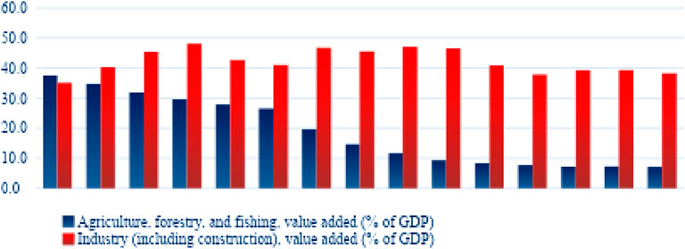
Figure 4. Agricultural and industrial sector revenues in China from 1962 to 2023 (World Bank, 2024a).

The transition from an agriculture-based economy to one characterized by intense industrialization necessitates the efficient and sustainable use of natural resources (Herman, 2024). Sustainable agricultural and fishing practices are vital for securing the production capacity to feed China’s large population and ensuring food security. Managing natural resources sustainably helps protect forest, agricultural, and marine ecosystems while maintaining biodiversity. Sustainable practices also support economic stability and growth in agriculture, forestry, and fisheries (Sharma et al., 2024).

China must develop and implement long-term strategies for the sustainable management of natural resources to ensure that the needs of future generations are met.

Policy actions concerning cropland, fishing, forests, and grazing are crucial for various SDGs, particularly Zero Hunger (SDG 2), Life Below Water (SDG 14), and Life on Land (SDG 15), while also indirectly influencing others like No Poverty (SDG 1) and Climate Action (SDG 13). Strengthening the supply chain, conserving natural resources, and preventing environmental degradation on land, in forests, and in marine environments are essential initiatives for promoting sustainability in all countries.

Due to its vast population, which constitutes approximately 17.72% of the global population, China’s unique position makes sustainable resource management critical. China’s substantial contribution to global meat, milk, and egg production (14%, 4.49%, and 36.83%, respectively) and its significant share in global fish and aquaculture production underscore the importance of sustainable practices for global food security in these sectors. Additionally, China is a major producer of softwood and hardwood, emphasizing the need for sustainable management of its forestry resources.

Given China’s role as a major agricultural producer and its massive transformation toward industrialization, sustainable management of its natural resources is crucial for national and global supply chains. The research aims to test the Environmental Kuznets Curve (EKC) and load capacity curve (LCC) hypotheses in China, focusing on cropland, fishing, forests, and grazing lands using Fourier bootstrap autoregressive distributed lag (ARDL) cointegration and FMOLS estimators with the Fourier function. With reference to all concepts evaluated in the study, the study provides comprehensive knowledge on sustainable agriculture and fishing using advanced econometric approaches. Focusing on the demand and supply sides of all relevant dependent variables plays a vital role in mitigating degradation and enriching productivity in terms of the EKC and LCC hypotheses; this study represents one of the first comprehensive investigations into the scope of sustainable agricultural and fishing. Moreover, Fourier bootstrap ARDL cointegration analysis provides more consistent results compared to the methods that ignore structural changes, and the FMOLS estimators confound the concerns of serial correlation and endogeneity by achieving asymptotic efficiency. Furthermore, the FMOLS estimators yield more reliable results in small samples and help eliminate bias caused by missing series. This study is a pioneering effort in separately focusing on all relevant ecological indicators to enhance understanding and policymaking in sustainable development.

Literature review

With the globalization process, discussions on the environment have increased. In this context, researchers have conducted many studies. The environmental issue was first associated with economic growth. The effects of economic growth on the environment have been addressed in numerous studies. In this context, the EKC hypothesis, which argues that there is an inverted U-shaped relationship between real GDP and CO₂ emissions, is frequently researched (Li et al., 2024; Aydin and Degirmenci, 2024). The validity of different forms of the EKC hypothesis has been investigated for various periods and countries. It has been observed that time series and panel data methodologies are used very frequently. In these studies, CO₂ emissions are generally preferred to represent environmental conditions. It has been determined that GDP per capita is used as the economic growth variable. Increased industrialization, high growth in global production, and the acceleration of liberalization steps have made foreign direct investments important. In this context, the relationship between foreign direct investments and the environment has begun to attract attention. Research has increasingly focused on the environment–foreign direct investment relationship. These studies tested the validity of the pollution haven and pollution halo hypotheses. The pollution haven hypothesis argues that foreign direct investment not only contributes positively to the economic development of developing countries but also forms the basis of environmental degradation experienced in these countries. On the other hand, the view that foreign direct investment reduces environmental degradation in developing countries supports the pollution halo hypothesis (Destek et al., 2024; Yilanci et al., 2023). In both hypotheses, the environmental variable is often represented by CO₂ emissions. The ecological footprint variable has recently begun to be used frequently among environmental indicators. On the other hand, recent studies have found that the load capacity factor (LCF) variable is rarely used. In addition to the EKC hypothesis, a new curve, the LCC), can be tested using the LCF. With LCC, it is argued that as income increases, environmental degradation initially increases, and above a certain income level, environmental degradation will decrease (Pata and Kartal, 2023).

Table 1 lists studies focusing on environmental degradation. In this context, the focus is on current research that tests the EKC, pollution halo, pollution haven, and LCC hypotheses.

Table 1

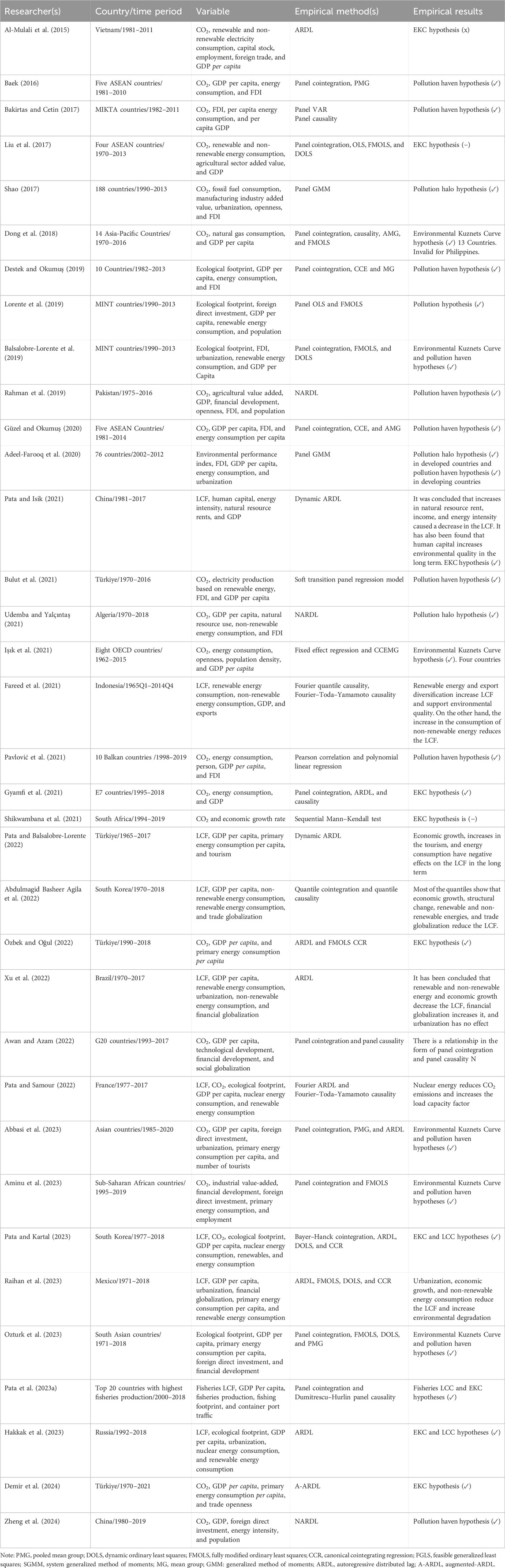
Table 1. Details of the literature.

When Table 1 is examined, it is observed that economic growth, foreign direct investment, and other socio-economic variables affect environmental degradation. Studies show that CO₂ emissions are the most commonly used indicator of environmental conditions. In a few studies, it has been found that the ecological footprint variable is preferred. The choice is influenced by the fact that the ecological footprint is a more comprehensive indicator than CO₂ emissions. On the other hand, it has been determined that the LCF variable is preferred in current studies. In this context, it stands out as an important variable for comparing results, especially in empirical studies. LCF, which monitors ecological thresholds by comparing biological capacity with the ecological footprint, enables comprehensive research on environmental degradation. Unlike CO₂ and the ecological footprint, an increase in the LCF indicates improved environmental quality (Pata and Isik, 2021). In contrast, CO₂ and the ecological footprint indicate degradation, while the LCF signals recovery (Pata and Kartal, 2023).

It has been determined that aside from the environmental variables in question, the most frequently used variable is energy consumption, along with economic growth and foreign direct investment. In this context, renewable or non-renewable energy consumption variables were preferred. The primary reason for this preference is that energy consumption from fossil fuels increases carbon emissions (Ghorbal et al., 2024; Li and Haneklaus, 2021; Hanif, 2018). When research on the validity of the EKC hypothesis is examined, the study by Grossman and Krueger (1991) is considered a pioneering work. The authors tested the validity of the EKC hypothesis using data from the economies of 42 countries for the period 1977–1988. The results of the study using the panel GLS method showed the validity of the relevant hypothesis. Under the leadership of this study, many studies have been conducted on the EKC hypothesis. These studies observed that in addition to the inverted U-shaped relationship, the N-shaped relationship has also been tested (Azam et al., 2024; Mohammed et al., 2024; Sarkodie and Ozturk, 2020). Thus, the course of the relationship between economic growth and the environment is determined periodically. In addition, turning points in relationships can be determined, and mathematical results can be produced. When the studies on the EKC Hypothesis in Table 1 are examined, it is understood that the results vary depending on the period, country, and empirical method used. However, in general, it was concluded that the relevant hypothesis was mostly valid. Interest in the pollution halo and pollution haven hypotheses increased in the periods following the introduction of the EKC hypothesis. Birdsall and Wheeler’s (1993) study on the validity of the pollution haven hypothesis is a pioneering study. The authors tested the validity of the relevant hypothesis in 25 Latin American countries during the 1960–1988 sample period. In the study where regression analysis was used as the empirical method, it was concluded that the pollution haven hypothesis is valid. In the following period, the relevant hypothesis was tested in numerous studies. Studies have shown that there has been an increase in the 2000s, when the globalization process deepened. Although foreign direct investment inflows were mostly used in the studies, foreign direct investment outflows were also preferred. Although there is no consensus on its validity, most findings support the pollution haven hypothesis. In the pollution haven hypothesis, as in the EKC Hypothesis, the results vary depending on the country, period, and empirical method used. It has been observed that the EKC and pollution haven hypotheses have been tested together in a limited number of recent studies (Aminu et al., 2023). This enables broader policy recommendations to be made regarding environmental degradation. Although results vary depending on the period, country, and method used, there are studies that support the validity of the EKC and pollution haven hypotheses together (Akkaya and Çetin, 2024; Pata et al., 2023b). In this study, where the effects of various variables on the environment are extensively examined, the EKC, pollution haven, and pollution halo hypotheses are examined in depth. On the other hand, recently, in addition to these hypotheses, there have been studies on LCC and fisheries LCC hypotheses, albeit in limited numbers (Raihan et al., 2023; Pata et al., 2023a). The main point in these studies is that the dependent variable used is LCF and its derivatives. In this context, it is observed that variables such as fishery LCF, GDP per capita, fishing production, fishing footprint, container port traffic, nuclear energy consumption, renewable energy consumption, foreign direct investment, urbanization, and financial development are used (Adalı et al., 2024; Wang et al., 2024). There is evidence in studies that financial development and foreign direct investments will increase environmental degradation by increasing economic development and energy consumption, suggesting that they may increase economic expansion and energy consumption and potentially harm the environment (Akinsola et al., 2022; Kihombo et al., 2021; Shahbaz et al., 2023).

Data and methodology

In order to provide the policy guidelines for various SDGs—directly Life on Land, Life Below Water, and Zero Hunger and indirectly for No poverty, Climate Action, and other SDGs— the EKC, LCC, the pollution haven, or halo hypotheses are analyzed. Urbanization, foreign trade openness, agriculture, forestry, and fishing value-added are included as the control variables within the framework of these hypotheses. Within this scope, this study employs an annual time series spanning from 1979 to 2022 by considering the availability of all used series. In the study, the cropland footprint, the fishing ground footprint, the forest products’ footprint, the grazing land footprint, and these series’ load capacity factors are utilized as the dependent variables. Using the series’ footprint and LCF data, this study provides comprehensive evidence on the demand and supply sides of the environmental indicators, contributing to holistic strategies for mitigating environmental degradation and enhancing sustainability.

Table 2 provides the characteristics and information on the variables. The study transforms all series into natural logarithm forms to calculate elasticity and ensure reliable and consistent results by mitigating heteroskedasticity. After providing the series details, Table 3 presents the descriptive analysis. According to the outcome of Table 3, the variable with the highest mean value is lnGDP, whereas the variable with the lowest value is lnGF. However, the highest standard deviation value is lnFDI.

Table 2

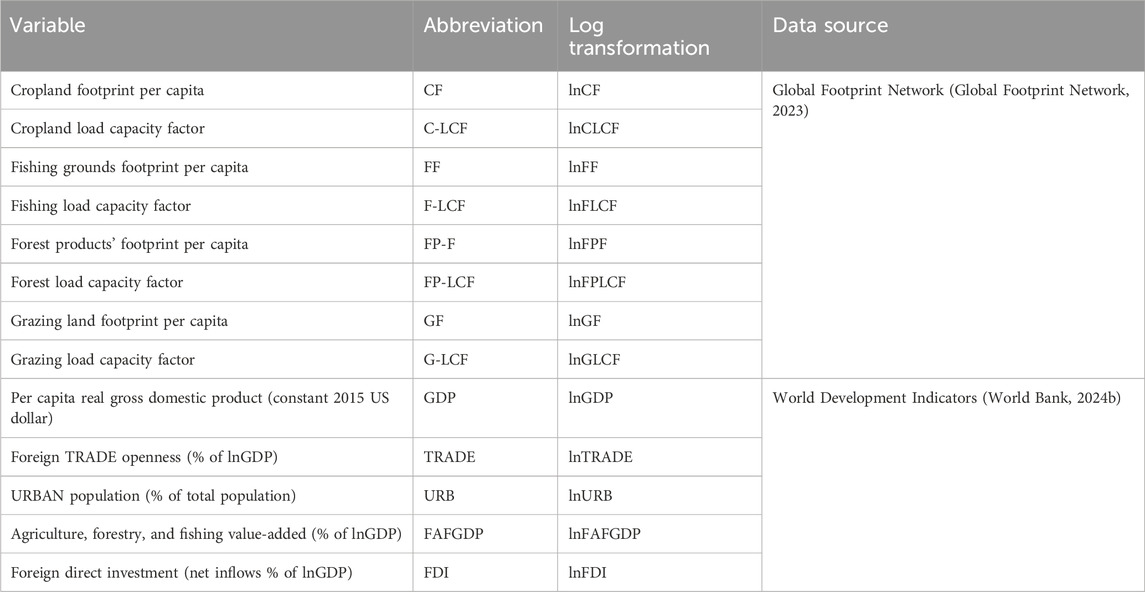
Table 2. Abbreviations and sources.

Table 3

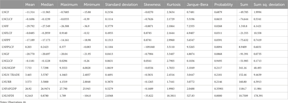
Table 3. Descriptive statistics.

In the study, the approach suggested by Narayan and Narayan is followed to test the EKC, LCF, and pollution haven/halo hypotheses. According to this approach, long-run income and LNFDI elasticity are first estimated; then, the short-run equation is derived using the residual terms from the long-run estimations, allowing the hypothesis to be evaluated by comparing long- and short-term elasticity. Focusing on the differences in the shape and interpretation of the EKC and LCF hypotheses, two model equations are demonstrated. The models for the footprints and LCFs of the series are shown in Equations 1, 2.

$\mathit{ln}{EF}_t=c_0+{\theta }_1{lnGDP}_t+{\theta }_2{lnFDI}_t+{\theta }_3{lncontrolvariable}_t+{ϵ}_t,(1)$

$\mathit{ln}{EF}_t=c_0+{\mathrm{\delta }}_1{lnGDP}_t+{\mathrm{\delta }}_2{lnFDI}_t+{\mathrm{\delta }}_t{lncontrolvariable}_t+{ϵ}_t.(2)$

In Equation 1, lnEF represents all footprint variables and lncontrol variables represent lnURB, lnLNTRADE, and lnFAFGDP, while $c_0$ and ${ϵ}_t$ are constant and the white noise terms, respectively. Moreover, ${\theta }_1$ and ${\theta }_2$ denote the long-run coefficient of lnGDP and lnFDI.

When performing the short-run estimations, comparing the short- and long-run coefficients of explanatory variables provides knowledge for testing the EKC and pollution haven/halo hypotheses. If long-term income and FDI elasticity are found to be lower than their short-run values, the presence of EKC and pollution halo hypotheses is confirmed. Because of the LCC hypothesis framework, if the long-term coefficients of lnGDP and lnFDI and the short-run coefficients of the considered variables are positive and negative, respectively, the LCC hypothesis is confirmed. After the preliminary analysis of the series, Figure 5 shows the steps for performing the econometric process in the study. Figure 5 reveals the methodology of the econometric methods.

Figure 5

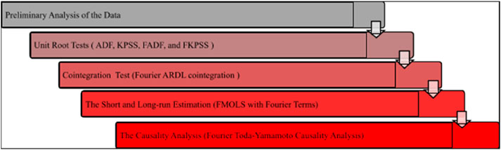
Figure 5. Econometric process.

Fourier bootstrap ARDL cointegration analysis

The conventional ARDL approach is one of the most widely used methods for testing the validity of the cointegration relationship between variables. When determining the presence of a cointegration connection between variables, two conditions stated by Pesaran et al. (2001) should be considered. First, the coefficient of the error correction terms and the lagged explanatory variables must be statistically significant in the ARDL model. Second, the lower and upper critical bounds test, as proposed by Pesaran et al. (2001), must be conducted.

However, executing upper and lower critical bounds is not necessary for the first condition as its validity relies on the order of integration of the variables. Suppose the variables considered in the model are cointegrated at I (1), confirming the first condition. In this case, the low power properties of conventional unit root tests should be taken into account (Goh et al., 2017). The conventional ARDL approach uses F- and t-statistics, and comparing these test statistics with the lower and upper bounds defined as I (0) and I (1), respectively, is essential for testing the validity of the cointegration connection. If the test statistics exceed the upper bound critical values, the null hypothesis indicating the absence of cointegration can be rejected. However, if the test statistics fall between the upper and lower bounds, it becomes inconclusive to determine the validity or absence of cointegration.

To address the limitations of the conventional ARDL approach, McNown et al. (2018) proposed employing bootstrap critical values, introducing an approach labeled as the bootstrap autoregressive distributed lag. When comparing the properties of the conventional and bootstrap ARDL approaches, it is claimed that the bootstrap ARDL approach provides more robust power properties than the conventional ARDL approach when multiple explanatory variables are present. Additionally, the bootstrap ARDL approach does not impose limitations on the order of integration of the series and is considered effective in correcting the weak power and size characteristics of conventional ARDL approaches (Pata and Aydın, 2020).

${∆lnX}_t={\theta }_0+{\displaystyle \sum _{i=1}^{p-1}}{\theta }_1{∆lnX}_{t-i}+{\displaystyle \sum _{i=1}^{z-1}}{\theta }_2{∆lnY}_{t-i}+{\displaystyle \sum _{i=1}^{k-1}}{\theta }_3{∆lnY}_{t-i}^2+{\displaystyle \sum _{i=1}^{k-1}}{\theta }_4{D}_{t,i}+{\gamma }_1{lnX}_{t-1}+{\gamma }_2{lnY}_{t-1}+{\gamma }_3{{lnY}^2}_{t-1}+{\mathrm{\mu }}_t.(3)$

In Equation 3, the constant terms are represented by ${\theta }_0$, while the short-term zero coefficients are denoted by ${\theta }_1$, ${\theta }_2$, and ${\theta }_3$. In addition, ${\gamma }_1$, ${\gamma }_2$, and ${\gamma }_3$ denote the long-term coefficients, while the dummy variables showing the sharp structural breaks are represented by $D_{t,i}$.

In order to determine the cointegration relationship between the variables, McKown et al. (2018) introduced novel test statistics for the lagged values of the independent variables, in addition to the F- and t-statistics. In this context, the overall F-statistic, t-dependent statistic for the lagged dependent variables, and the newly introduced F-independent statistic for the lagged independent variables are employed to test the null hypothesis. The null hypothesis employed for these three statistics are shown in Equations 4-6 as follows:

$F_{statistic}\to H_0={\gamma }_1={\gamma }_2={\gamma }_3=0,(4)$

$T_{dependent}\to H_0={\gamma }_1=0,(5)$

$F_{statistic}\to H_0={\gamma }_1={\gamma }_2={\gamma }_3=0.(6)$

Later, the bootstrap ARDL test is augmented with Fourier terms, as developed by Solarin (2019), and the fractional frequency flexible Fourier forms are incorporated into the bootstrap ARDL approach proposed by Yilanci et al. (2020). Overall, if the three test statistics considered are simultaneously greater than the measured bootstrap critical values, the null hypothesis should be rejected, confirming the existence of a cointegration relationship between the variables.

FMOLS estimators with the Fourier function

The fully modified ordinary least squares (FMOLS) estimator, proposed by Phillips and Hansen (1990), is regarded as one of the most effective and reliable estimators because most estimators face issues such as serial correlation and endogeneity, which impair the consistent estimation of regressors. The FMOLS estimator overcomes these problems by achieving asymptotic efficiency and provides more consistent results in small samples. Additionally, FMOLS estimators eliminate the bias caused by missing series.

Although FMOLS estimators generate long-run coefficients, short-run estimators can also be derived using the residual terms from the long-run estimation as error correction (EC) terms and employing the first-difference values of the series under consideration. Furthermore, when FMOLS estimators are augmented with the Fourier function, the Fourier FMOLS estimators can be obtained, enabling estimation while accounting for smooth structural breaks.

Fourier Toda–Yamamoto causality analysis

The conventional Toda–Yamamoto (T-Y) causality analysis, introduced by Toda and Yamamoto (1995), is one of the most widely used causality analyses in the literature for detecting causality connections between variables. The T-Y causality analysis relies on the vector autoregressive (VAR) models of Sims (1980) and provides more robust information compared to the Granger causality analysis as it uses the level values of the variables, thereby avoiding long-run information loss.

In T-Y causality analysis, the optimal lag length is determined by considering the lag based on the VAR model (denoted as p) and the maximum order of integration of the series (represented as d_max). Thus, p + d_max represents the optimal lag length used in the T-Y causality analysis. Additionally, the T-Y causality analysis is regarded as a flexible method because prior information on unit root and cointegration properties is not required.

However, the T-Y causality analysis assumes that the constant term remains stable over time and that structural changes do not impact the series’ data generation process.

Neglecting structural changes, including various properties such as unknown numbers, dates, and smooth or sharp transitions, may lead to biased or misleading rejections of the null hypothesis.

In this context, Enders and Jones (2016) emphasized that failing to account for structural changes in VAR models can produce inaccurate and inconsistent evidence of causal connections. To address this, researchers have utilized the Fourier function in VAR models, leading to the development of the Fourier Granger (FG) causality analysis. Nazlioglu et al. (2016) extended this by incorporating the Fourier function into the T-Y causality analysis, introducing the Fourier Toda–Yamamoto (FTY) causality analysis. By integrating the Fourier function, the FTY causality analysis accounts for smooth structural breaks and mitigates long-run information loss, enhancing the robustness of causality detection. Furthermore, the single-frequency FTY causality analysis is expressed in Equation 7.

$m_t={\alpha }_0+{\alpha }_1{m}_{t-1}+\dots \dots +{\alpha }_{{p+d}_{\mathit{max}}}{m_t}_{-\left({p+d}_{\mathit{max}}\right)}+{\gamma }_1\sin \left(\frac{2k\pi t}{T}\right)+{\gamma }_2\cos \left(\frac{2k\pi t}{T}\right)+{\mu }_t.(7)$

In Equation 7, $m_t$ denotes the vector containing the considered series, while ${p+d}_{\mathit{max}}$ represents the optimal lag of the VAR model and the maximum order of the integration of the series. The Fourier terms’ parameters are represented by ${\gamma }_1$ and ${\gamma }_2$, while k, π, and t denote the frequencies, pi-values, and trend, respectively. The white noise error terms are represented by ${\mathrm{\mu }}_t$. The null hypothesis of the FTY posing the absence of causality ($H_0$: ${\alpha }_1$ = … = ${\alpha }_{\mathrm{p}}$ = 0) is tested against the alternative hypothesis ($H_a$: ${\alpha }_1=\dots ={\alpha }_{\mathrm{p}}$ ≠ 0).

Results

Before performing the cointegration analysis, short- and long-run estimations, and causality analysis to find evidence for the EKC, LCC, and pollution haven or halo hypotheses regarding the Chinese environmental indicators, a stationary analysis should be executed to examine whether the considered series are stationary at the level and determine the degree of integration among the series. The stochastic properties of the series are crucial for applying econometric approaches.

To achieve this, the conventional ADF and KPSS unit root tests with a constant, and a constant and trend, as well as the Fourier ADF (FADF) introduced by Enders and Lee (2012) and Fourier KPSS (FKPSS) proposed by Christopoulos and León-Ledesma (2010), are performed. The unit root tests with a constant, and a constant and trend are applied. In this study, the primary unit root tests are the FADF and FKPSS unit root tests, which allow for the consideration of multiple smooth, unknown, and sharp structural changes if the trigonometric functions are detected to be significant. The significance of the trigonometric functions is determined by comparing the values of the F-test statistics with the critical values of the F-test. Critical values of the F-test, obtained from Becker et al. (2006), are shown in the notes of Table 4, and the F-test statistics are presented in the second set of square brackets. The first set of square brackets represents the structural changes. If the F-test statistics exceed the critical values, the FADF and FKPSS results are interpreted. However, if a controversial case is identified, the conventional ADF and KPSS unit root tests are considered.

Table 4

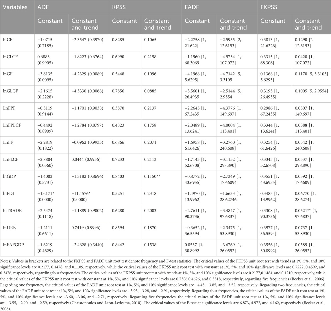
Table 4. Unit root test results for the variables at the level.

The unit root test results for the series at the level and the first differences are tabulated in Table 4 and Table 5, respectively.

Table 5

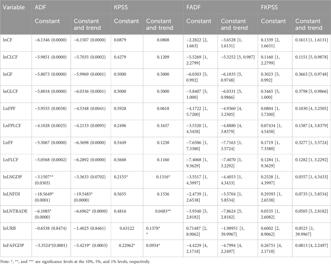
Table 5. Unit root test results for the variables at the first differences.

In the study, the environmental proxies consisting of lnCF, cropland-LCF, fishing-EF, fishing-LCF, forest-EF, forest-LCF, grazing-EF, and grazing-LCF are initially examined to determine their stochastic pattern. When comparing the F-test statistics with the critical values of the F-tests, it is observed that the trigonometric terms are significant in all series, except for the results of the FADF and FKPSS unit root tests with a constant and trend on grazing-EF and grazing-LCF. However, the findings of the mentioned tests with a constant confirm the significance of the trigonometric terms in the considered series.

The FADF and FKPSS unit root tests confirm that lnCF contains unit roots, and the FADF and FKPSS unit root tests with a constant show that lnCLCF is not stationary, while the tests with a constant and trend indicate that lnCLCF is stationary at the level.

Fishing-EF and fishing-LCF have unit roots at the level as a result of the FADF and FKPSS unit root tests.

With respect to the results obtained from the FADF unit root test with a constant and the FKPSS unit root tests concerning forest-EF and forest-LCF, the series are not stationary at the series’ level values. Grazing-EF and grazing-LCF show a unit root as a result of the FADF and FKPSS unit root tests with constant, while the ADF and FKPSS unit root tests with a constant and trend show that the series is stationary. The FADF and FKPSS unit root tests with a constant confirm that forest-EF and forest-LCF are not stationary, whereas the tests with a constant and trend provide controversial findings, verifying the stationarity of the series.

When examining the outcome of the unit root tests on the remaining series of the considered independent variables, the first difference values of the series become stationary.

After performing the stationary analysis, the next step in the empirical approach is conducting a cointegration analysis to examine whether the variables considered in the models are cointegrated or not. If the cointegration relationship between the variables in the different models is verified, the long- and short-run effects of the independent variables on the environmental indicators, including the ecological footprint and load capacity factors of cropland, fishing grounds, forest products, and grazing land, are examined to test the EKC and LCC hypotheses, as well as the pollution halo/haven hypothesis, by considering three control variables: lnTRADE, lnURB, and lnFAFGDP. The bootstrap Fourier ARDL cointegration analysis is performed for each considered model.

The bootstrap Fourier ARDL cointegration analysis reports three statistical values: Fa, t-dependent, and Fb. The null hypothesis for these three tests indicates the absence of cointegration and assumes that the test statistics are significant and greater than the table’s critical values. If this is the case, the null hypothesis is rejected, and the cointegration relationship between the variables in the model is confirmed.

In this context, the cropland ecological footprint (CF) and the cropland load capacity factors (C-LCFs) are the first considered dependent variables examined in models (1–6). The findings of the bootstrap Fourier ARDL cointegration analysis are shown in Table 6. Upon reviewing Table 6, it is concluded that the null hypothesis for all three tests should be rejected, and the test statistics are significant and exceed the critical values in all generated models where C-LCF is the dependent variable. In contrast, the long-run connection is confirmed in the first and second models, where CF is the dependent variable, while the null hypothesis is not rejected in the third model, where lnFAFGDP is used as the control variable.

Table 6

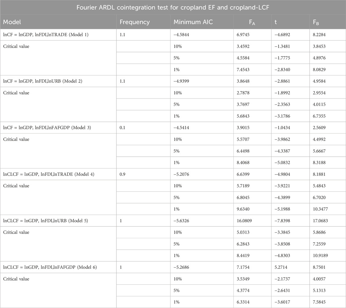
Table 6. Results of Fourier bootstrap ARDL cointegration results for the cropland footprint and cropland load capacity factor.

The Fourier ARDL cointegration analysis confirms the presence of the cointegrated connection among variables in all models on lnCF and lnC-LCF, except Model 3. Therefore, the short- and long-run estimations are investigated using Fourier estimation with the Fourier functions. The logarithmic forms of the series are considered in the long-run estimations, and the first difference forms of the series are employed in the short-run estimations. EC parameters are obtained from the residual of the long-run estimations, and optimal lags used in Fourier functions are determined as a result of the Fourier ARDL cointegration analysis. Suppose the short- and long-run coefficients of lnGDP are detected as positive and negative, respectively, or the short-run negative coefficient of lnGDP is higher than the long-run negative coefficient. In this case, the EKC hypothesis with lnCF is verified. Regarding the C-LCC hypothesis, the expected nexus between lnGDP and lnCLCF is reversed, considering the previously mentioned relationship with lnCF. The effect of lnFDI on lnCF and lnCLCF is found to be positive and negative, respectively, confirming the validity of the pollution haven hypothesis.

These theoretically expected relationships hold for the remaining generated models. In light of this explanation, the short- and long-run estimations for Model 1, Model 2, Model 4, Model 5, and Model 6 are presented in Table 7.

Table 7

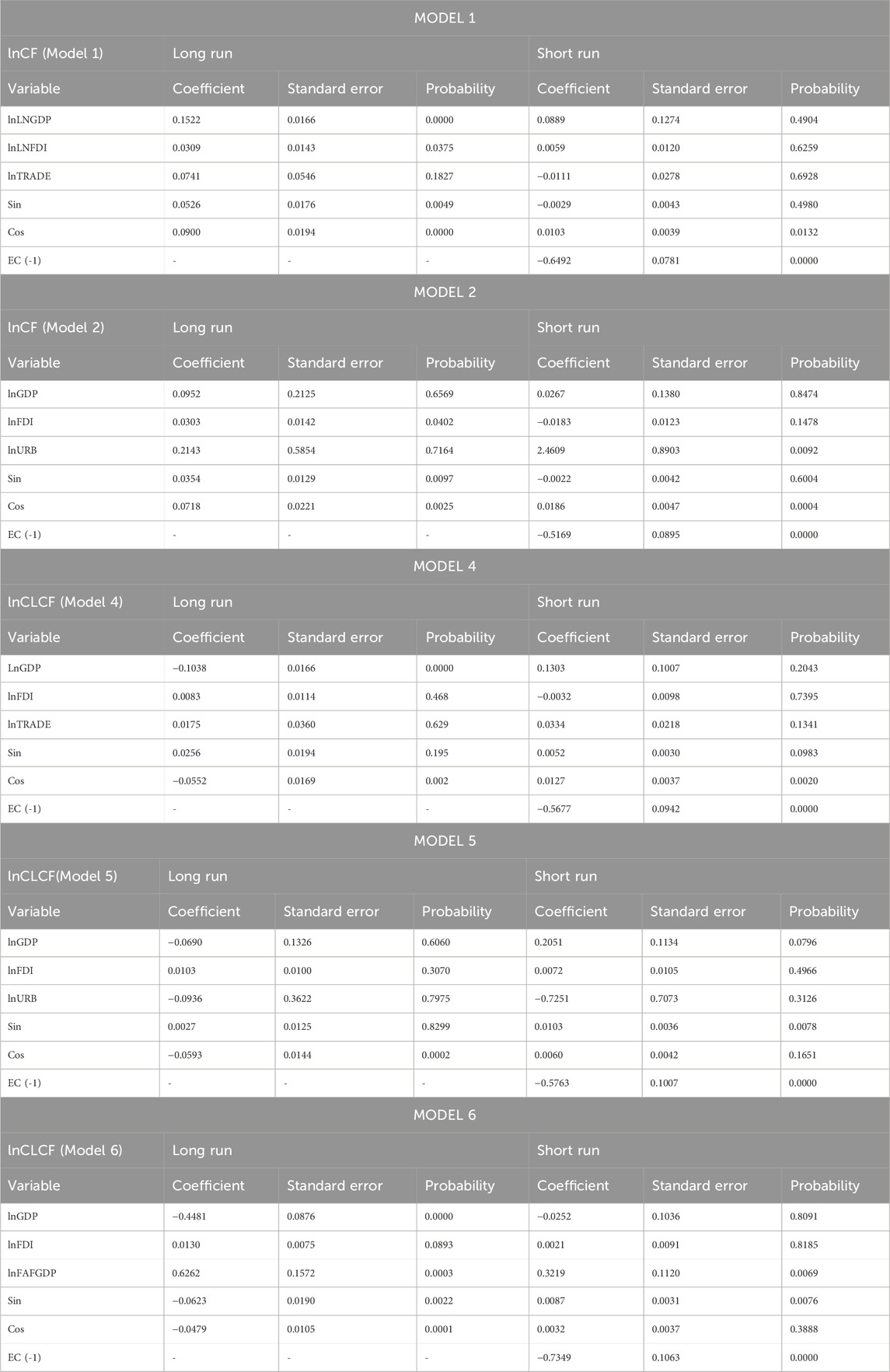
Table 7. Short- and long-run estimations for models 1, 2, 4, 5, and 6.

According to Table 7 presenting Model 1, none of the considered independent variables have a significant influence on lnCF, but the coefficient of EC is found to be negative and significant, and the cosine term is also statistically significant. In the long-run estimations, the pollution haven hypothesis is confirmed, indicating that an increase in lnGDP contributes to higher pressure on cropland degradations. However, the Fourier term is statistically significant.

Table 7, which presents the results of Model 2, shows that lnGDP does not a statistically significant impact on lnCF in the short and long run. The outcome of Model 2 supports the pollution haven hypothesis as a 1% increase in lnFDI leads to a 0.030% increases in lnCF. Furthermore, lnCF is positively influenced by lnURB in the short run by 2.46%, which implies that lnURB is a factor harming the cropland-related environment.

When scrutinizing Table 7’s finding concerning Model 4, all explanatory variables are not statistically significant in the short run. On the other hand, lnGDP is the only explanatory variable in the long run, promoting a statistically significant impact on lnCLCF. In addition, the C-LCC hypothesis is not confirmed because decreasing cropland quality is associated with increased lnGDP.

Table 7, which presents the results of Model 5, shows the short and-long-run coefficients of the explanatory variables in lnCLCF. The result of the short-run estimation claims that lnGDP has an improved influence on lnCLCF, while the remaining variables are not statistically significant. Regarding the result of the long-run estimations, lnCLCF does not correspond with all explanatory variables.

The final evidence concerning lnCLCF is achieved from Model 6, and the estimations’ outcome is shown in Table 7. The pollution halo hypothesis holds for China when examining the nexus between lnFDI and lnCLCF in the long run. At the same time, lnFAFGDP is detected as an essential improved factor of lnCLCF in the short and long run. On the other hand, the C-LCC hypothesis does not exist when focusing on the result of Model 6 as a 1% increase in lnGDP impairs lnCLCF by a calculated 0.44%.

The result of the Fourier Toda–Yamamoto causality analysis concerning lnCF and lnCLCF is provided in Table 8. The null hypothesis indicating the absence of the causality is rejected when the bootstrap p-values are lower than the significance level. The causality nexus between the explanatory variables and lnCF is first interpreted, and later, the lnCLCF is considered. According to Table 8, the mutual causality link between lnURB and lnCF is detected at a 10% significance level, and a one-way causality connection operating from lnCF to lnFAFGDP is also indicated. Regarding the results on the causality nexus between the explanatory variables and lnCLCF, a mutual causality connection between lnFAFGDP and lnCLCF is verified.

Table 8

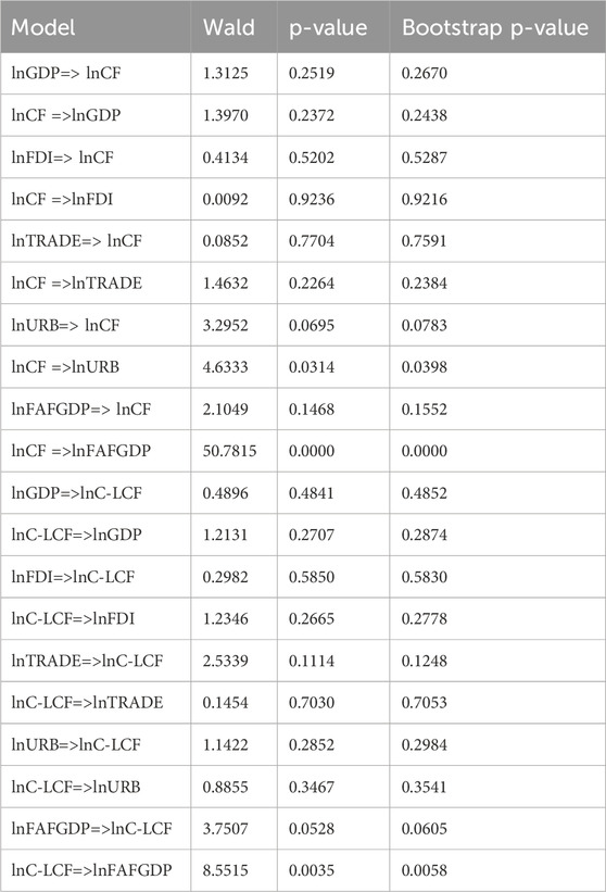
Table 8. Result of the Fourier–Toda–Yamamoto causality analysis on the cropland footprint and cropland load capacity factor.

The demand and supply sides of the fishing stocks are crucial for sustainability because the marine ecosystem plays a vital role in providing fisheries while regulating and balancing all ecosystem segments. The FGF related to the demand side of the marine ecosystem, while the fishing grounds-load capacity factors (FG-LCFs) reflect its supply side, and the effects of economic growth and LNFDI are examined, considering foreign lnTRADE, lnURBanization, and lnFAFGDP as control variables. According to the stochastic properties of the variables confirming the same cointegrated order I (1), the bootstrap Fourier ARDL cointegration analysis is employed on the fishing-related models. The outcome of the cointegration analysis is displayed in Table 9. According to Table 9, the cointegration relations hold for models 9 and 10 due to the rejection of the null hypothesis of three tests at a 10% significance level. In contrast, t-dependent and Fb test statistics reveal the validity of the long-run movement in models 8 and 12. Furthermore, the Fa test statistics are only significant for Model 7 at a 10% significance level. The absence of the cointegration connections is found for Model 11 due to three tests.

Table 9

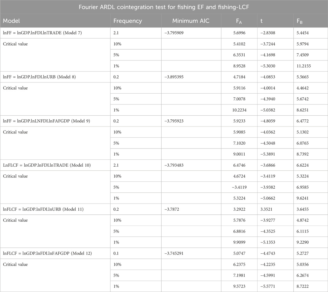
Table 9. Results of Fourier bootstrap ARDL cointegration results for the fishing grounds footprint and fishing load capacity factor.

After confirming the validity of the long-run movement in all fishing-based models except Model 11, short- and long-run estimations are applied to the considered models. Table 9 presents the findings on Model 7, revealing that all independent variables are statistically significant at a 10% significance level in the short run. In contrast, only lnLNTRADE has a substantial impact on fishing-EF in the long run, contributing to a reduction in fishing-related degradation. However, lnTRADE exacerbates fishing-related degradation in the short run, which is calculated as 0.15%, while the pollution halo hypothesis is valid. Furthermore, an increase in lnLNGDP contributes to higher pressure on the fishing ecosystem in the short run. However, the Fourier terms and EC are statistically significant only in the short run. Table 10 presents the result of Model 8, indicating that fishing-EF is not statistically associated with the considered independent variables in the short run.

Table 10

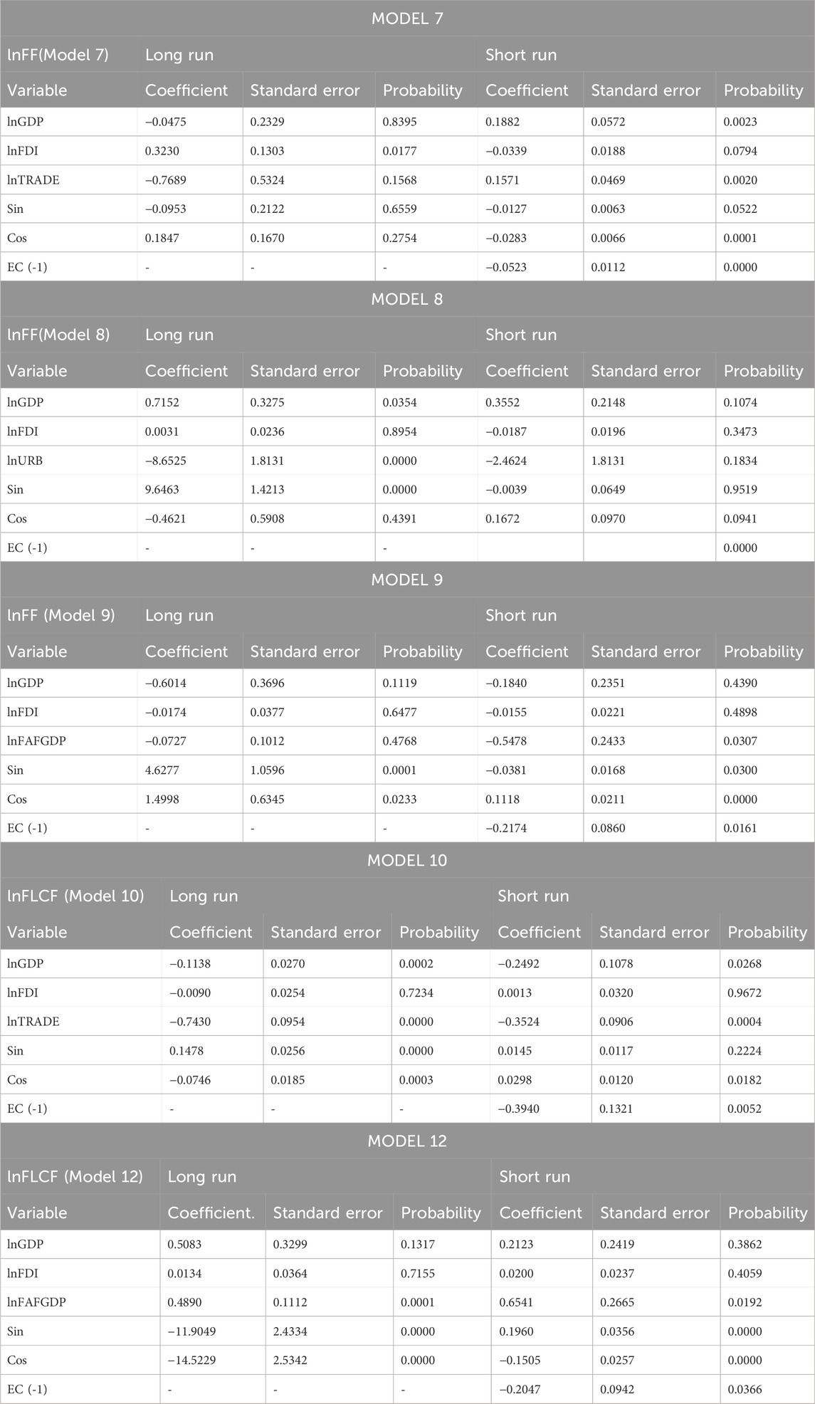
Table 10. Short- and long-run estimations for models 7, 8, 9, 10, and 12.

As for the long-run estimations, fishing-EF is positively and negatively induced by lnLNGDP and lnURB, respectively. According to the outcome of the long- and short-run estimation concerning Model 9, lnLNGDP and lnLNFDI statistically matter for fishing-EF in the short and long run, while lnFAFGDP promotes a favorable impact on the fishing-related ecosystem in the short run, which is calculated as 0.54%. However, Table 10 confirms the significance of the Fourier terms in the short and long run and the theoretical expectation of EC. When considering the demand and supply sides of the fishing ecosystem, Table 10 shows evidence of Model 10 in which lnLNTRADE is used as a control variable under the F-LCF and the pollution haven or halo hypothesis. When examining the results of Table 10, F-LCF is not statistically influenced by lnLNFDI in the short and long run.

At the same time, F-LCF is deteriorated by a 1% increase in lnLNTRADE in the short and long run, detected as 0.35% and 0.74%, respectively. However, the F-LCC hypothesis is valid in Model 10 because the unfavorable impact of lnLNGDP on F-LCF reduces over time. According to the findings of Table 10, which presents the results of Model 12, lnLNGDP and lnFDI are not statistical determinants of F-LCF in the short and long run. Moreover, the short- and long-run lnFAFGDP coefficients are measured at 0.65% and 0.48%, respectively, which underlines the enriched role of lnFAFGDP in F-LCF. However, the Fourier terms are statistically significant as a result of the short- and long-run estimations, and EC is measured at a negative and significant level of 5%. In light of this explanation, the short- and long-run estimations concerning Model 7, Model 8, Model 9, Model 10, and Model 12 are provided in Table 10.

Table 11 presents the evidence concerning the causality link between the explanatory variables and fishing-related indicators. The findings indicate that fishing-EF is caused by lnLNFDI, and, in turn, fishing-EF induces lnLNTRADE. Moreover, lnLNFDI is also an inducing factor of fishing-LCF.

Table 11

Table 11. Result of the Fourier–Toda–Yamamoto causality analysis on the fishing grounds and fishing load capacity factor.

Table 12 documents the bootstrap Fourier ARDL cointegration test result of the generated models in which the forest products’ footprint and the forest-load capacity factors are the dependent variables. Examining the outcome of the analysis for Model 13, it is concluded that the measured test statistics for Fa, t-dependent, and Fb are greater than the critical values at a 5% significance level, and all three hypotheses are not accepted. This finding proves the cointegration relationship among lnFPF, lnLNGDP, lnLNFDI, and lnLNTRADE. Regarding Model 14, the calculated test statistics of three hypotheses induce all three null hypotheses to be accepted, and the cointegration connection between the variables in Model 14 is not confirmed. When inquiring about the outcome related to Model 15, the test statistics of Fa and Fb are not greater than the critical values. In contrast, the calculated t-dependent statistics are significant at a 5% significance level. Therefore, the long-run movement holds for Model 16. Regarding the Fourier bootstrap ARDL cointegration results for Model 16, Fa and t-dependent measured test statistics exceed the critical values at all significance levels, while the Fb test statistics are significant at a 5% significance level, and all three null hypotheses of the tests are rejected. The long-run relationship is confirmed for Model 16. Considering the result for Model 17, it is underlined that all three null hypotheses are not accepted at a 5% significance level and that the validity of the cointegrated connection is important for the variables in Model 17. Finally, when considering the outcome of Model 18, it is concluded that Fa t-dependent and Fb test statistics are not sufficient to reject the null hypothesis. The validity of the cointegrated relationship is not verified in Model 18.

Table 12

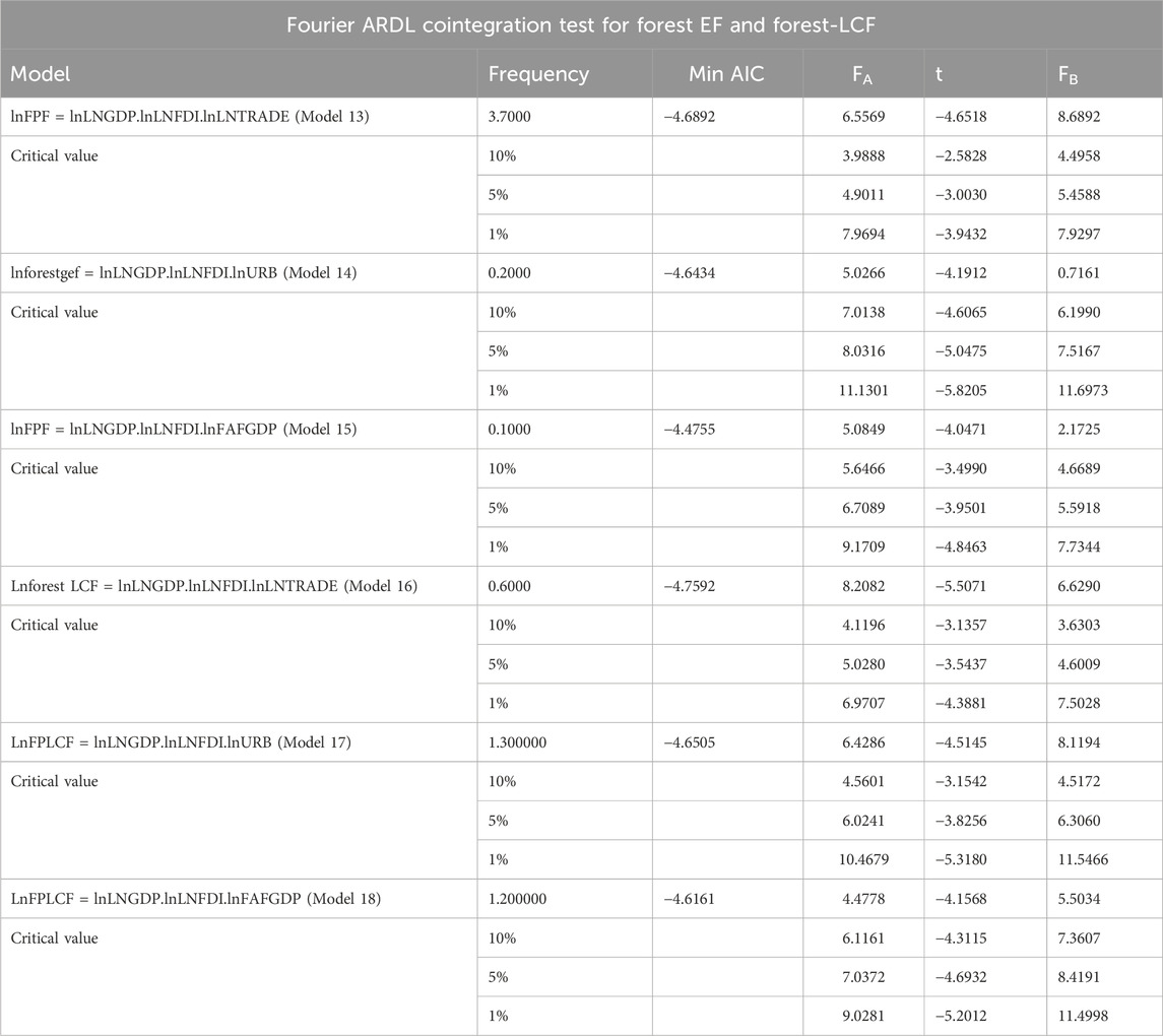
Table 12. Fourier bootstrap ARDL cointegration results for the forest products’ footprint and the forest-load capacity factor.

Following the validity of the cointegration relationship between the variables in Model 13, the study’s objective is to examine the EKC hypothesis and the pollution halo/haven, along with considering the effect of lnLNTRADE on the FPF. FMOLS estimations with the Fourier function investigate the short- and long-run coefficients of lnLNGDP, lnLNFDI, and lnLNTRADE on the FPF. The result of the FMOLS estimations is displayed in Table 13. When observing the result on the short run of the FMOLS estimations, the EKC hypothesis with the FPF is not verified because an increase in lnLNGDP impairs the forest degradation, and the long-run coefficient of lnLNGDP is greater than its short-run coefficient. The coefficient of lnLNFDI is not statistically significant in the short run. In contrast, a 1% increase in lnLNFDI is associated with a 0.08% increase in forest degradation, which verifies the presence of the pollution haven. Moreover, forest degradation increases with an increase in lnLNTRADE, and the negative effect of lnLNTRADE on forest degradation is more pronounced in the long run. In addition, the cointegrated connection holds for Model 15, where lnFAFGDP is employed as a control variable under investigation for the EKC and pollution halo/heaven hypotheses. The result of the FMOLS estimations with the Fourier function is provided in Table 13. The coefficients of lnLNGDP and lnLNFDI are statistically insignificant in the short and long run. At the same time, lnFAFGDP exacerbates in the long run. The forest products’ load capacity factors (FP-LCFs) are employed to test their LCC (FP-LCF) hypothesis. The FP-LCF hypothesis can be examined in models 16 and 17, where the long-run movement among the variables is confirmed. The outcome of Model 16 is presented in Table 13, and the forest-related quality is influenced by lnLNGDP measured at 0.20%, while the worst effect of lnLNGDP on the FP-LCF is calculated as 0.11%. The FP-LCF hypothesis exists in China. In the long run, lnLNFDI reduces the forest quality, and the pollution haven hypothesis is presented. However, lnTRADE is an improved factor in enhancing FP-LCF. The FP-LCC and pollution haven/halo hypotheses are investigated considering lnURB as a control variable in Model 17. The finding of the FMOLS estimation on Model 17 is shown in Table 13. As revealed in the short-run result, FP-LCF is statistically not induced by lnLNGDP, lnLNFDI, and lnURB. The coefficient of lnLNFDI is also reported as insignificant in the long run, but lnLNGDP and lnLNTRADE are statistically appropriate to interpret. A 1% increase in lnLNGDP corresponds to a 0.56% decrease in the FP-LCF, while lnURB leads to an increase in the FP-LCF, calculated as 1.28%. In light of this explanation, the short- and long-run estimations for Model 13, Model 15, Model 16, and Model 17 are provided in Table 13.

Table 13

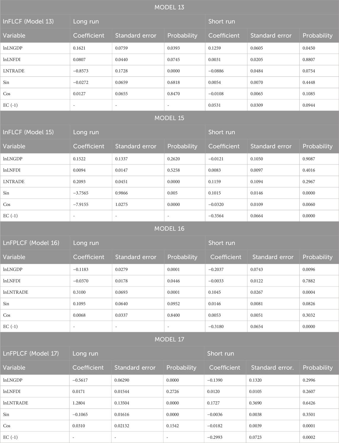
Table 13. Short- and long-run estimations for models 13, 15, 16, and 17.

The findings from the Fourier–Toda–Yamamoto causality analysis concerning the nexus between explanatory variables and forest-related environmental indicators are presented in Table 14. These findings indicate that the forest-EF and forest-LCF are not statistically induced by all explanatory variables.

Table 14

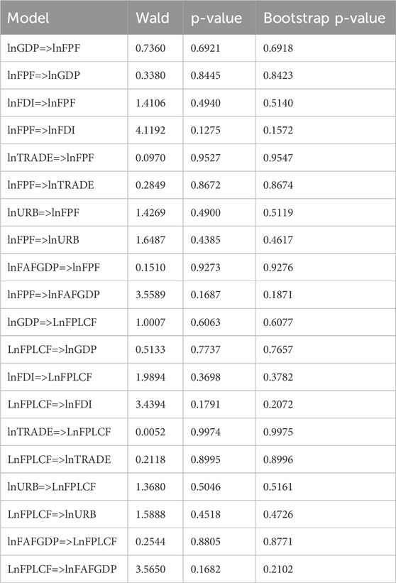
Table 14. Results of Fourier–Toda–Yamamoto causality analysis for the forest products’ footprint and forest load capacity factor.

Other environmental indicators concerning the food supply, land, and marine sustainability are the grazing land footprint (GLF) and the grazing land-load capacity factors (G-LCF). Another objective of the study is to examine the effect of economic growth and LNFDI, along with control variables, on GLF and G-LCF. The stationary analysis reveals that all variables become stationary at the first differences; in other words, they are integrated at I (1). Then, the bootstrap Fourier ARDL cointegration test is also processed to examine the validity of the cointegration connection. When evaluating all results shown in Table 15 for the models numbered from 19 to 24, it is highlighted that the null hypothesis, meaning the absence of the long-run relationship between the variables of Fa, t-dependent, and Fb, is rejected at a 10% significance level because the test statistics at the absolute value are greater than the critical values.

Table 15

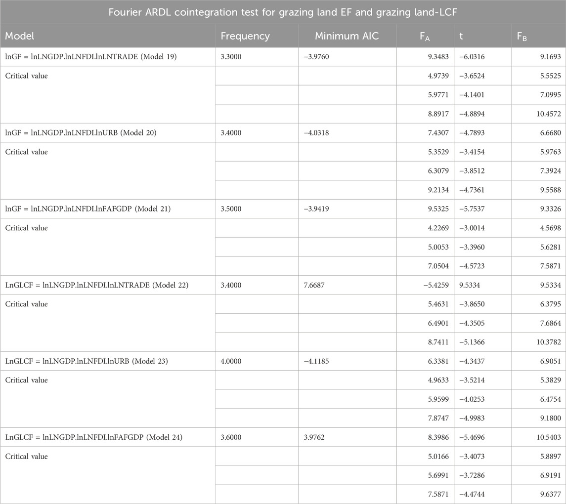
Table 15. Fourier bootstrap ARDL cointegration results for the grazing land footprint and the grazing land load capacity factor.

As the long-run connection is verified for all grazing land footprint and grazing-load capacity factor-based models, the long- and short-run effect of the independent variables on grazing-EF and grazing-LCF is examined using FMOLS estimators with Fourier terms. Table 16 presents the result concerning Model 19, and the outcome of the estimation shows that lnLNGDP and Fourier terms are not statistically significant in the short and long run. In contrast, the pollution haven hypothesis is confirmed in the long run at a 5% significance level, whereas the coefficient of LNFDI is found to be insignificant in the short run. The role of lnTRADE in grazing-related environmental degradation has varied over time. A 1% increase in lnTRADE in long and short run induces approximately a 0.43% decrease and a 0.093% increase in grazing-related environmental degradation. However, the value of EC is positive and statistically insignificant.

Table 16

Table 16. Short- and long-run estimations for models 19, 20, 21, 22, 23, and 24.

Table 16 discloses the outcome of the estimation of Model 20. According to Table 16, the EKC hypothesis is not verified because the long- and short-run effect of lnLNGDP on the grazing-EF is found to be impaired. Expanding economic activities in the long run induces more pressure on the grazing land than in the short run. The pollution haven hypothesis holds for China in the long run, while lnURBanization plays a pivotal role in mitigating environmental degradation.

Moreover, the coefficient of EC is negative and significant at a 1% significance level, while Fourier terms are not statistically significant in the short and long run. Regarding lnFAFGDP being used as a control variable, the cointegration analysis confirms the long-run movement between variables, so short- and long-run estimations are performed. The outcome of the FMOLS estimation with the Fourier terms is presented in Table 16. According to Table 16, the EKC hypothesis is verified as the long-run coefficient of lnLNGDP is lower than that of the short-run at a 10% significance level. However, lnLNFDI deteriorates the environmental quality in the long run, which supports the presence of the pollution haven hypothesis. At the same time, an increase in lnFAFGDP promotes an enriched impact on environmental quality in the short and long run.

Table 16 reveals the short- and long-run effects of the considered determinants on G-LCF. When considering the results of Model 22, it is concluded that only lnLNGDP is statistically significant, and a 1% increase in lnLNGDP leads to a 0.031% decrease in G-LCF. Furthermore, Table 16 discloses the evidence concerning Model 23, and the G-LCC hypothesis is demonstrated because the adverse impact of lnLNGDP on the G-LCF seems to have shrunk over time. G-LCF is not statistically associated with lnLNFDI in the short and long run. However, lnURB plays an essential role in enhancing G-LCF. The result of Model 24 is similar to the finding of Model 23; in other words, the G-LCC hypothesis is also verified, and the neutrality hypothesis with the nexus between LNFDI and G-LCF is detected. Furthermore, a 1% increase in lnFAFGDP in the short and long run leads to an improvement in G-LCF, measured as 0.29 and 0.011, respectively. In light of this explanation, the short- and long-run estimations concerning Model 19, Model 20, Model 21, Model 22, Model 23, and Model 24 are provided in Table 16.

The results of Fourier–Toda–Yamamoto causality analysis for the grazing land footprint and grazing load capacity factor are documented in Table 17. The causality connection between the considered independent variables and grazing-related environmental indicators is detected as a one-way causality link operating from lnURB to G-EF, and G-EF induces lnLNTRADE. Moreover, the results of Fourier Toda–Yamamoto analysis on G-LCF indicate that lnURB causes G-LCF and lnLNTRADE is influenced by G-LCF.

Table 17

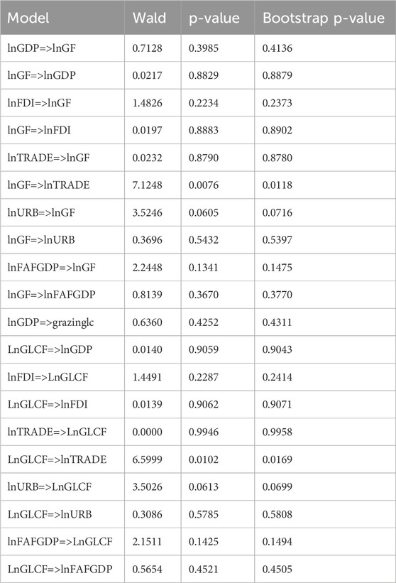
Table 17. Results of Fourier–Toda–Yamamoto causality analysis for the grazing land footprint and grazing load capacity factor.

Discussion and conclusion

This study analyzes the effect of economic growth and foreign direct investment on the SDG targets Zero Hunger (2), Life Below Water (14), and Life on Land (15) by examining relevant sub-components of ecological footprint and load capacity factors have been analyzed within the framework of EKC and LCC hypotheses in China. Cropland, fishing, forest, and grazing land are considered environmental areas, and foreign trade (lnTRADE), urbanization (lnURBAN), agriculture, forestry, and fishing are considered control variables. To achieve this objective, the study employs Fourier bootstrap ARDL cointegration analysis and FMOLS estimators, expanded with the Fourier function.

The CF and C-LCF are the first environmental indicators considered for the study’s objective. The long-run relationship holds for all models except Model 3 on CF, where lnFAFGDP is used as a control variable under the EKC hypothesis. When examining the results concerning the nexus between lnFDI and lnCF, the pollution haven hypothesis is verified in the long run. Furthermore, lnCF is not influenced by lnTRADE, while lnURB promotes an increased impact on lnCF in the short run. The pressure on the cropland-related environment factors is accelerated by lnGDP, so the EKC hypothesis on lnCF does not hold for China as a result of analysis on all models. Regarding the outcome of lnC-LCF, it is underlined that the C-LCC hypothesis does not exist, and lnGDP impairs the C-LCF in models 4 and 6. In addition, the role of lnFDI, lnTRADE, and lnURB in lnC-LCF are found to be insignificant, while lnFAFGDP plays an enriched role in cropland sustainability. Although the study mainly concentrates on the indicators related to Life on Land to provide policy direction concerning Zero Hunger and other SDG targets, the sustainable marine ecosystem also plays a pivotal role in the success of SDGs. According to the evidence obtained from the investigation on the considered models, lnURB and lnFAFGDP are found to mitigate fishing degradations, whereas the effect of lnFDI on lnFF varies over time—negative in the short run, confirming the pollution halo hypothesis, and positive in the long run, verifying the pollution haven hypothesis. In addition, fishing degradation is accelerated by an increase in lnGDP, which induces the rejection of the F-EKC hypothesis. The F-LCC hypothesis is confirmed when considering the estimations found in Model 10, but the results in Model 12 indicate an insignificant connection between lnGDP and lnF-LCF. Moreover, lnFDI also does not matter for fishing sustainability. However, fishing sustainability is improved by lnFAFGDP. The FP and FP-LCF are essential indicators, especially in Life on Land, SDG Target 15, and others. As a consequence of the investigation of six models based upon lnFP and lnFP-LCF, it is revealed that the EKC hypothesis is not valid as the short and long run of lnGDP accelerate lnFP, and lnFAFGDP and lnFDI are identified as other impaired factors. As for the evidence on lnFP-LCF, lnURB and lnTRADE are improved factors in forest sustainability, and FP-LCC hypothesis is also confirmed. At the same time, the negative connection between lnFDI and lnFP-LCF in Model 16 is detected. The GF and G-LCF are China’s final considered environmental indicators in terms of providing guidelines on a sustainable food supply chain. Along with the method applied to remaining environmental indicators, six different models are considered, i.e, three models related to GF and the remaining three models related to G-LCF; these models examine the control variables within the framework of the EKC, LCC, and pollution haven or halo hypotheses. When examining the effect of lnFDI and lnGDP on GF, the pollution haven hypothesis is verified in all three models, while the EKC hypothesis is not confirmed. In the long run, all control variables comprising lnURB, lnTRADE, and lnFAFGDP promote a favorable influence in mitigating grazing degradations. In contrast, when scrutinizing the dynamic role of lnLNGDP in G-LCF, the G-LCC hypothesis holds for China, while lnFDI and lnTRADE do not influence the G-LCF. Moreover, lnurn and lnFAFGDP play a pivotal role in improving G-LCF.

Accompanying the summary of the empirical findings on all considered models, the reliable policy directions aim to mitigate the pressure of human activities on the CF, FF, FP-F, and GF and enhance the biocapacity of the considered environmental indicators. LCF plays a vital role in various SDGs, including Zero Hunger (2), Life Below Water (14), and Life on Land (15) and indirectly contributes to the remaining SDGs. With respect to the function of lnFDI in Chinese sustainability, the pollution haven hypothesis is verified for most of the considered models. China is one of the leading FDI-inflow hubs in the world. Still, the legal framework, norms, regulations, and attitude toward the environment are not sufficient to support the evidence on the pollution haven hypothesis in the study. Policymakers may reshape and enact FDI-related policies that provide subsidies, tax exemptions, and facilities for profit transfer, management, and production for firms enacted with modern management methods and cutting-edge technologies. In addition, exemptions on electricity and energy costs and reducing the red tape are vital policy measures to counteract the negative effects of FDI on the environment. When the lnGDP influences the environmental indicators, the Chinese economic structure is not harmonized with sustainability. China’s economic welfare is achieved at the cost of environmental degradation, characterized by high energy intensity, a significant share of nonrenewable energy resources in total energy, and the use of polluting technologies and production methods. Improving energy efficiency, enhancing renewable energy transitions, and public and government partnerships to stimulate greener technology and energy are essential policies transforming polluted economic performance into sustainability. On the other hand, the role of lnTRADE is detected as an improved factor for Chinese sustainability, which implies that China has been transforming from labor-intensity and low-tech goods into capital-intensity and high-tech goods such as semiconductors. Urbanization process and income from fishing and agriculture sectors are found to be enriched factors in China. In order to maximize the benefits of these fields, policy initiatives should be prioritize green and cutting-edge technologies, management strategies, and production methods, such as employing shallow geothermal energy in agriculture, heating and cooling systems, and pro-environmental building methods across all sectors of the Chinese economy.

Furthermore, the study encountered limitations that have yet not been addressed. First, the study provides only the evidence for China regarding related areas’ sustainability, whereas focusing on wide-panel samples or different aspects of the importance of local cases should be investigated. Moreover, varied social, political, and macroeconomic indicators are other options for further studies.

Data availability statement

Publicly available datasets were analyzed in this study. These data can be found at: https://www.footprintnetwork.org. https://databank.worldbank.org/source/world-development-indicators.

Author contributions

İG: conceptualization, data curation, formal analysis, investigation, methodology, project administration, resources, software, supervision, validation, visualization, writing–original draft, and writing–review and editing. MN: conceptualization, data curation, formal analysis, investigation, methodology, project administration, resources, software, supervision, validation, visualization, writing–original draft, and writing–review and editing. OŞ: conceptualization, data curation, formal analysis, investigation, methodology, project administration, resources, software, supervision, validation, visualization, writing–original draft, and writing–review and editing. ZA: supervision, validation, visualization, writing–original draft, writing–review and editing, conceptualization, data curation, formal analysis, investigation, methodology, project administration, resources, and software. SÖ: conceptualization, data curation, formal analysis, investigation, methodology, project administration, resources, software, supervision, validation, visualization, writing–original draft, and writing–review and editing.

Funding

The author(s) declare that no financial support was received for the research, authorship, and/or publication of this article.

Acknowledgments

All authors have read and agreed to the published version of the manuscript.

Conflict of interest

The authors declare that the research was conducted in the absence of any commercial or financial relationships that could be construed as a potential conflict of interest.

Generative AI statement

The author(s) declare that no Generative AI was used in the creation of this manuscript.

Publisher’s note

All claims expressed in this article are solely those of the authors and do not necessarily represent those of their affiliated organizations, or those of the publisher, the editors and the reviewers. Any product that may be evaluated in this article, or claim that may be made by its manufacturer, is not guaranteed or endorsed by the publisher.

References

Abbasi, M. A., Nosheen, M., and Rahman, H. U. (2023). An approach to the pollution haven and pollution halo hypotheses in Asian countries. Environ. Sci. Pollut. Res. 30 (17), 49270–49289. doi:10.1007/s11356-023-25548-x

PubMed Abstract | CrossRef Full Text | Google Scholar

Abdulmagid Basheer Agila, T., Khalifa, W. M., Saint, A. S., Adebayo, T. S., and Altuntaş, M. (2022). Determinants of load capacity factor in South Korea: does structural change matter? Environ. Sci. Pollut. Res. 29 (46), 69932–69948. doi:10.1007/s11356-022-20676-2

CrossRef Full Text | Google Scholar

Adalı, Z., Toygar, A., Karataş, A. M., and Yıldırım, U. (2024). Sustainable fisheries and the conservation of marine resources: a stochastic analysis of the fishery balance of African countries. J. Nat. Conserv. 80, 126653. doi:10.1016/j.jnc.2024.126653

CrossRef Full Text | Google Scholar

Adeel-Farooq, R. M., Riaz, M. F., and Ali, T. (2020). Improving the environment begins at home: revisiting the links between FDI and environment. Energy 215 (Part B), 1–29. doi:10.1016/j.energy.2020.119150

CrossRef Full Text | Google Scholar

Akinsola, G. D., Awosusi, A. A., Kirikkaleli, D., Umarbeyli, S., Adeshola, I., and Adebayo, T. S. (2022). Ecological footprint, public-private partnership investment in energy, and financial development in Brazil: a gradual shift causality approach. Environ. Sci. Pollut. Res. 29 (7), 10077–10090. doi:10.1007/s11356-021-15791-5

PubMed Abstract | CrossRef Full Text | Google Scholar

Akkaya, F., and Çetin, M. A. (2024). Çevresel Kuznets eğrisi ve kirlilik sığınağı hipotezleri gelişmekte olan ülkeler için geçerli midir? ÇAKÜ SBED 15 (1), 29–60. doi:10.54558/jiss.1218992

CrossRef Full Text | Google Scholar

Al-Mulali, U., Saboori, B., and Öztürk, İ. (2015). Investigating the environmental Kuznets curve hypothesis in Vietnam. Energy Policy 76, 123–131. doi:10.1016/j.enpol.2014.11.019

CrossRef Full Text | Google Scholar

Aminu, N., Clifton, N., and Mahe, S. (2023). From pollution to prosperity: investigating the environmental Kuznets curve and pollution-haven hypothesis in sub-Saharan Africa's industrial sector. J. Environ. Manage 342, 118147. doi:10.1016/j.jenvman.2023.118147

PubMed Abstract | CrossRef Full Text | Google Scholar

Awan, A. M., and Azam, M. (2022). Evaluating the impact of GDP per capita on environmental degradation for G-20 economies: does N-shaped environmental Kuznets curve exist? Environ. Dev. Sustain 24 (9), 11103–11126. doi:10.1007/s10668-021-01899-8

CrossRef Full Text | Google Scholar

Aydin, M., and Degirmenci, T. (2024). The role of greenfield investment and investment freedom on environmental quality: testing the EKC hypothesis for EU countries. Int. J. Sustain Dev. World Ecol. 31, 684–694. doi:10.1080/13504509.2024.2326567

CrossRef Full Text | Google Scholar

Azam, M., Rehman, Z. U., Khan, H., and Haouas, I. (2024). Empirical testing of the environmental Kuznets curve: evidence from 182 countries of the world. Environ. Dev. Sustain, 1–36. doi:10.1007/s10668-024-04890-1

CrossRef Full Text | Google Scholar

Baek, J. (2016). A new look at the FDI-income-energy-environment nexus: dynamic panel data analysis of ASEAN. Energy Policy 91, 22–27. doi:10.1016/j.enpol.2015.12.045

CrossRef Full Text | Google Scholar

Bakirtas, I., and Cetin, M. A. (2017). Revisiting the environmental Kuznets curve and pollution haven hypotheses: MIKTA sample. Environ. Sci. Pollut. Res. 24, 18273–18283. doi:10.1007/s11356-017-9462-y

PubMed Abstract | CrossRef Full Text | Google Scholar

Balsalobre-Lorente, D., Gokmenoglu, K. K., Taspinar, N., and Cantos-Cantos, J. M. (2019). An approach to the pollution haven and pollution halo hypotheses in MINT countries. Environ. Sci. Pollut. Res. 26, 23010–23026. doi:10.1007/s11356-019-05446-x

PubMed Abstract | CrossRef Full Text | Google Scholar

Becker, R., Enders, W., and Lee, J. (2006). A stationarity test in the presence of an unknown number of smooth breaks. J. Time Ser. Anal. 27 (3), 381–409. doi:10.1111/j.1467-9892.2006.00478.x

CrossRef Full Text | Google Scholar

Bhattarai, K., and Adhikari, A. P. (2023). Promoting urban farming for creating sustainable cities in Nepal. Urban Sci. 7 (2), 54. doi:10.3390/urbansci7020054

CrossRef Full Text | Google Scholar

Birdsall, N., and Wheeler, D. (1993). Trade policy and industrial pollution in Latin America: where are the pollution havens? J. Environ. Dev. 2 (1), 137–149. doi:10.1177/107049659300200107

CrossRef Full Text | Google Scholar

Bulut, Ü., Üçler, G., and Inglesi-Lotz, R. (2021). Does the pollution haven hypothesis prevail in Turkey? Empirical evidence from nonlinear smooth transition models. Environ. Sci. Pollut. Res. 28, 38563–38572. doi:10.1007/s11356-021-13476-7

PubMed Abstract | CrossRef Full Text | Google Scholar

Caradus, J. R., Chapman, D. F., and Rowarth, J. S. (2024). Improving human diets and welfare through using herbivore-based foods: 2. Environmental consequences and mitigations. Animals 14 (9), 1353. doi:10.3390/ani14091353

PubMed Abstract | CrossRef Full Text | Google Scholar

Christopoulos, D. K., and León-Ledesma, M. A. (2010). Smooth breaks and non-linear mean reversion: post-Bretton Woods real exchange rates. J. Int. Money Finance 29 (6), 1076–1093. doi:10.1016/j.jimonfin.2010.02.003

CrossRef Full Text | Google Scholar

Demir, O., Uludağ, K., and Özdemir, D. (2024). Testing the environmental Kuznets curve using the augmented boundary test (A-ARDL) in Türkiye: period 1970-2021. J. Econ. Adm. Sci. 25 (1), 81–95. doi:10.37880/cumuiibf.1334231

CrossRef Full Text | Google Scholar

Destek, M. A., and Okumuş, I. (2019). Does pollution haven hypothesis hold in newly industrialized countries? Evidence from ecological footprint. Environ. Sci. Pollut. Res. 26, 23689–23695. doi:10.1007/s11356-019-05614-z

PubMed Abstract | CrossRef Full Text | Google Scholar

Destek, M. A., Yıldırım, M., and Manga, M. (2024). High-income developing countries as pollution havens: can financial development and environmental regulations make a difference? J. Clean. Prod. 436, 140479. doi:10.1016/j.jclepro.2023.140479

CrossRef Full Text | Google Scholar

Dong, K., Sun, R., Li, H., and Liao, H. (2018). Does natural gas consumption mitigate CO₂ emissions: testing the environmental Kuznets curve hypothesis for 14 Asia-Pasific countries. Renew. Sustain Energy Rev. 94, 419–429. doi:10.1016/j.rser.2018.06.026

CrossRef Full Text | Google Scholar

Enders, W., and Jones, P. (2016). Grain prices, oil prices, and multiple smooth breaks in a VAR. Stud. Nonlinear Dyn. E. 20 (4), 399–419. doi:10.1515/snde-2014-0101

CrossRef Full Text | Google Scholar

Enders, W., and Lee, J. (2012). The flexible Fourier form and Dickey–Fuller type unit root tests. Econ. Lett. 117 (1), 196–199. doi:10.1016/j.econlet.2012.04.081

CrossRef Full Text | Google Scholar

Fareed, Z., Salem, S., Adebayo, T. S., Pata, U. K., and Shahzad, F. (2021). Role of export diversification and renewable energy on the load capacity factor in Indonesia: a Fourier quantile causality approach. Front. Environ. Sci. 9, 770152. doi:10.3389/fenvs.2021.770152

CrossRef Full Text | Google Scholar

Food and Agriculture Organization of the United Nations (2024). Statistics. Available online at: https://www.fao.org/statistics/en.

Google Scholar

Ghorbal, S., Soltani, L., and Ben Youssef, S. (2024). Patents. fossil fuels, foreign direct investment, and carbon dioxide emissions in South Korea. Environ. Dev. Sustain 26 (1), 109–125. doi:10.1007/s10668-022-02770-0

CrossRef Full Text | Google Scholar

Global Footprint Network (2023). Footprint data foundation. Available online at: https://www.footprintnetwork.org.

Google Scholar

Goh, S. K., Sam, C. Y., and McNown, R. (2017). Re-examining foreign direct investment, exports, and economic growth in Asian economies using a bootstrap ARDL test for cointegration. J. Asian Econ. 51, 12–22. doi:10.1016/j.asieco.2017.06.001

CrossRef Full Text | Google Scholar

Grossman, G. M., and Krueger, A. B. (1991). Environmental impacts of a north American free trade agreement. NBER Work Pap. Ser. 3914, 1–39. doi:10.3386/w3914

CrossRef Full Text | Google Scholar

Güzel, A. E., and Okumuş, I. (2020). Revisiting the pollution haven hypothesis in ASEAN-5 countries: new insights from panel data analysis. Environ. Sci. Pollut. Res. 27, 18157–18167. doi:10.1007/s11356-020-08317-y

PubMed Abstract | CrossRef Full Text | Google Scholar

Gyamfi, B. A., Adedoyin, F. F., Bein, M. A., and Bekun, F. V. (2021). Environmental implications of N-shaped environmental Kuznets curve for E7 countries. Environ. Sci. Pollut. Res. 28 (25), 33072–33082. doi:10.1007/s11356-021-12967-x

PubMed Abstract | CrossRef Full Text | Google Scholar

Hakkak, M., Altintaş, N., and Hakkak, S. (2023). Exploring the relationship between nuclear and renewable energy usage, ecological footprint, and load capacity factor: a study of the Russian Federation testing the EKC and LCC hypothesis. Renew. Energy Focus 46, 356–366. doi:10.1016/j.ref.2023.07.005

CrossRef Full Text | Google Scholar

Hanif, I. (2018). Impact of fossil fuels energy consumption, energy policies, and urban sprawl on carbon emissions in East Asia and the Pacific: a panel investigation. Energy Strat. Rev. 21, 16–24. doi:10.1016/j.esr.2018.04.006

CrossRef Full Text | Google Scholar

Hasan, M. M., and Du, F. (2023). The role of foreign trade and technology innovation on economic recovery in China: the mediating role of natural resources development. Resour. Policy 80, 103121. doi:10.1016/j.resourpol.2022.103121

PubMed Abstract | CrossRef Full Text | Google Scholar

Henn, D., Duffy, C., Humphreys, J., Gibbons, J., Byrne, K. A., and Styles, D. (2024). Cattle production strategies to deliver protein with less land and lower environmental impact. J. Environ. Manage 356, 120569. doi:10.1016/j.jenvman.2024.120569

PubMed Abstract | CrossRef Full Text | Google Scholar

Herman, E. (2024). Sustainable agriculture and its impact on the rural development in EU countries: a multivariate analysis. Land 13 (7), 947. doi:10.3390/land13070947

CrossRef Full Text | Google Scholar

Işık, C., Ongan, S., Özdemir, D., Ahmad, M., Irfan, M., Alvarado, R., et al. (2021). The increases and decreases of the Environment Kuznets Curve (EKC) for 8 OECD countries. Environ. Sci. Pollut. Res. 28, 28535–28543. doi:10.1007/s11356-021-12637-y

PubMed Abstract | CrossRef Full Text | Google Scholar

Kemp, P. S., Subbiah, G., Barnes, R., Boerder, K., O’Leary, B. C., Stewart, B. D., et al. (2023). The future of marine fisheries management and conservation in the United Kingdom: lessons learnt from over 100 years of biased policy. Mar. Policy 147, 105075. doi:10.1016/j.marpol.2022.105075

CrossRef Full Text | Google Scholar

Kihombo, S., Ahmed, Z., Chen, S., Adebayo, T. S., and Kirikkaleli, D. (2021). Linking financial development, economic growth, and ecological footprint: what is the role of technological innovation? Environ. Sci. Pollut. Res. 28 (43), 61235–61245. doi:10.1007/s11356-021-14993-1

PubMed Abstract | CrossRef Full Text | Google Scholar

Klimovskikh, N., Sekerin, V., Makushkin, S., Kuzmicheva, A., Leontev, M., and Kochetkov, E. (2023). Impact of human resource management on improving the innovation potential of an enterprise to achieve the principles of sustainable development. J. Law Sustain Dev. 11 (1), e0274. doi:10.37497/sdgs.v11i1.274

CrossRef Full Text | Google Scholar

Li, B., and Haneklaus, N. (2021). The role of renewable energy. fossil fuel consumption, urbanization and economic growth on CO₂ emissions in China. Energy Rep. 7, 783–791. doi:10.1016/j.egyr.2021.09.194

CrossRef Full Text | Google Scholar

Li, S., Jiao, J., Degen, A. A., Wang, W., Qi, T., Huang, M., et al. (2024). Cooperative management can mitigate trade-offs between livestock production and ecological functions to promote grassland sustainability. Agric. Ecosyst. Environ. 370, 109057. doi:10.1016/j.agee.2024.109057

CrossRef Full Text | Google Scholar

Liu, X., Zhang, S., and Bae, J. (2017). The impact of renewable energy and agriculture on carbon dioxide emissions: investigating the Environmental Kuznets Curve in four selected ASEAN countries. J. Clean. Prod. 164, 1239–1247. doi:10.1016/j.jclepro.2017.07.086

CrossRef Full Text | Google Scholar

Lorente, D. B., Gökmenoğlu, K. K., Taşpınar, N., and Cantos-Cantos, J. M. (2019). An approach to the pollution haven and pollution halo hypotheses in MINT countries. Environ. Sci. Pollut. Res. 26, 23010–23026. doi:10.1007/s11356-019-05446-x

CrossRef Full Text | Google Scholar

McKown, A. D., Klápště, J., Guy, R. D., El-Kassaby, Y. A., and Mansfield, S. D. (2018). Ecological genomics of variation in bud-break phenology and mechanisms of response to climate warming in Populus trichocarpa. New Phytol. 220 (1), 300–316. doi:10.1111/nph.15273

PubMed Abstract | CrossRef Full Text | Google Scholar

McNown, R., Sam, C. Y., and Goh, S. K. (2018). Bootstrapping the autoregressive distributed lag test for cointegration. Appl. Econ. 50 (13), 1509–1521. doi:10.1080/00036846.2017.1366643

CrossRef Full Text | Google Scholar

Mohammed, S., Gill, A. R., Ghosal, K., Al-Dalahmeh, M., Alsafadi, K., Szabó, S., et al. (2024). Assessment of the environmental kuznets curve within EU-27: steps toward environmental sustainability (1990–2019). Environ. Sci. Ecotech 18, 100312. doi:10.1016/j.ese.2023.100312

PubMed Abstract | CrossRef Full Text | Google Scholar

Naghdi, S., Rezaei, M., Heidari, M. G., Tahergorabi, R., Lorenzo, J. M., and Mirzaei, F. (2024). Insights into fishery by-product application in aquatic feed and food: a review. Aquac. Int. 32, 5851–5910. doi:10.1007/s10499-024-01447-x

CrossRef Full Text | Google Scholar

Nazlioglu, S., Gormus, N. A., and Soytas, U. (2016). Oil prices and real estate investment trusts (REITs): gradual-shift causality and volatility transmission analysis. Energy Econ. 60, 168–175. doi:10.1016/j.eneco.2016.09.009

CrossRef Full Text | Google Scholar

Özbek, S., and Oğul, B. (2022). Çevresel Kuznets eğrisi hipotezinin geçerliliği: Türkiye üzerine ampirik bir çalışma. AKAD 14 (26), 35–46. doi:10.20990/kilisiibfakademik.1041209

CrossRef Full Text | Google Scholar

Ozturk, I., Farooq, S., Majeed, M. T., and Skare, M. (2023). An empirical investigation of financial development and ecological footprint in South Asia: bridging the EKC and pollution haven hypotheses. Geosci. Front. 15, 101588. doi:10.1016/j.gsf.2023.101588

CrossRef Full Text | Google Scholar

Pata, U. K., Ahmed, Z., Eryilmaz, S., Zeren, F., and Gencer, Y. G. (2023b). Analyzing the environmental Kuznets curve for transportation modes in European countries. Transp. Res. D. Transp. Environ. 122, 103893. doi:10.1016/j.trd.2023.103893

CrossRef Full Text | Google Scholar

Pata, U. K., and Aydın, M. (2020). Testing the EKC hypothesis for the top six hydropower energy-consuming countries: evidence from Fourier Bootstrap ARDL procedure. J. Clean. Prod. 264, 121699. doi:10.1016/j.jclepro.2020.121699

CrossRef Full Text | Google Scholar

Pata, U. K., and Balsalobre-Lorente, D. (2022). Exploring the impact of tourism and energy consumption on the load capacity factor in Turkey: a novel dynamic ARDL approach. Environ. Sci. Pollut. Res. 29 (9), 13491–13503. doi:10.1007/s11356-021-16675-4

PubMed Abstract | CrossRef Full Text | Google Scholar

Pata, U. K., and Isik, C. (2021). Determinants of the load capacity factor in China: a novel dynamic ARDL approach for ecological footprint accounting. Resour. Policy 74, 102313. doi:10.1016/j.resourpol.2021.102313

CrossRef Full Text | Google Scholar

Pata, U. K., and Kartal, M. T. (2023). Impact of nuclear and renewable energy sources on environment quality: testing the EKC and LCC hypotheses for South Korea. Nucl. Eng. Technol. 55 (2), 587–594. doi:10.1016/j.net.2022.10.027

CrossRef Full Text | Google Scholar

Pata, U. K., Kartal, M. T., Adali, Z., and Karlilar, S. (2023a). Proposal of fishing load capacity curve and testing validity: evidence from top 20 countries with highest fisheries production by panel data approaches. Ocean. Coast Manag. 245, 106856. doi:10.1016/j.ocecoaman.2023.106856

CrossRef Full Text | Google Scholar

Pata, U. K., and Samour, A. (2022). Do renewable and nuclear energy enhance environmental quality in France? A new EKC approach with the load capacity factor. Prog. Nucl. Energy 149, 104249. doi:10.1016/j.pnucene.2022.104249

CrossRef Full Text | Google Scholar

Pavlović, A., Njegovan, M., Ivanišević, A., Radišić, M., Takači, A., Lošonc, A., et al. (2021). The impact of foreign direct investments and economic growth on environmental degradation: the case of the Balkans. Energies 14 (3), 566. doi:10.3390/en14030566

CrossRef Full Text | Google Scholar

Pesaran, M. H., Shin, Y., and Smith, R. J. (2001). Bounds testing approaches to the analysis of level relationships. J. Appl. Econom. 16 (3), 289–326. doi:10.1002/jae.616

CrossRef Full Text | Google Scholar

Phillips, P. C., and Hansen, B. E. (1990). Statistical inference in instrumental variables regression with I (1) processes. Rev. Econ. Stud. 57 (1), 99–125. doi:10.2307/2297545

CrossRef Full Text | Google Scholar

Rahman, Z. U., Chongbo, W., and Ahmad, M. (2019). An (a)symmetric analysis of the pollution haven hypothesis in the context of Pakistan: a non-linear approach. Carbon Manag. 10 (3), 227–239. doi:10.1080/17583004.2019.1577179

CrossRef Full Text | Google Scholar

Raihan, A., Rashid, M., Voumik, L. C., Akter, S., and Esquivias, M. A. (2023). The dynamic impacts of economic growth, financial globalization, fossil fuel, renewable energy, and urbanization on load capacity factor in Mexico. Sustainability 15 (18), 13462. doi:10.3390/su151813462

CrossRef Full Text | Google Scholar

Renyong, H., and Sedik, A. A. (2023). Environmental sustainability and foreign direct investment in east Africa: institutional and policy benefits for environmental sustainability. Sustainability 15 (2), 1521. doi:10.3390/su15021521

CrossRef Full Text | Google Scholar

Rosenfeld, T., Pokorny, B., Marcovitch, J., and Poschen, P. (2024). Bioeconomy based on non-timber forest products for development and forest conservation-untapped potential or false hope? A systematic review for the Brazilian Amazon. For Policy Econ 163, 103228. doi:10.1016/j.forpol.2024.103228

CrossRef Full Text | Google Scholar

Sarkodie, S. A., and Ozturk, I. (2020). Investigating the environmental Kuznets curve hypothesis in Kenya: a multivariate analysis. Renew. Sustain Energy Rev. 117, 109481. doi:10.1016/j.rser.2019.109481

CrossRef Full Text | Google Scholar

Shahbaz, M., Dogan, M., Akkus, H. T., and Gursoy, S. (2023). The effect of financial development and economic growth on ecological footprint: evidence from top 10 emitter countries. Environ. Sci. Pollut. Res. 30 (29), 73518–73533. doi:10.1007/s11356-023-27573-2

PubMed Abstract | CrossRef Full Text | Google Scholar

Shao, Y. (2017). Does FDI affect carbon intensity? New evidence from dynamic panel analysis. Int. J. Clim. Chang. Str. Manag. 10 (1), 27–42. doi:10.1108/IJCCSM-03-2017-0062

CrossRef Full Text | Google Scholar

Sharma, I., and Birman, S. (2024). “Biodiversity loss. ecosystem services. and their role in promoting sustainable health,” in The climate-health-sustainability nexus: understanding the interconnected impact on populations and the environment. Editors P. Singh, and N. Yedav (Champaign, Switzerland: Springer Nature), 163–188.

CrossRef Full Text | Google Scholar

Shikwambana, L., Mhangara, P., and Kganyago, M. (2021). Assessing the relationship between economic growth and emissions levels in South Africa between 1994 and 2019. Sustainability 13 (5), 2645. doi:10.3390/su13052645

CrossRef Full Text | Google Scholar

Sims, C. A. (1980). Macroeconomics and reality. Econometrica 48 (1), 1–48. doi:10.2307/1912017

CrossRef Full Text | Google Scholar

Soeparna, I. I., and Taofiqurohman, A. (2024). Transversal policy between the protection of marine fishery resources and fisheries subsidies to address overfishing in Indonesia. Mar. Policy 163, 106112. doi:10.1016/j.marpol.2024.106112

CrossRef Full Text | Google Scholar

Solarin, S. A. (2019). Modelling the relationship between financing by Islamic banking system and environmental quality: evidence from bootstrap autoregressive distributive lag with Fourier terms. Qual. Quant. 53 (6), 2867–2884. doi:10.1007/s11135-019-00904-7

CrossRef Full Text | Google Scholar

Statista (2024). Forest industry in China - statistics and facts. Available online at: https://www.statista.com/topics/11409/forestry-in-china/.

Google Scholar

Sugiawan, Y., Kurniawan, R., and Managi, S. (2023). Assessing the United Nations sustainable development goals from the inclusive wealth perspective. Sci. Rep. 13 (1), 1601. doi:10.1038/s41598-023-29318-0

PubMed Abstract | CrossRef Full Text | Google Scholar

Tampekis, S., Kantartzis, A., Arabatzis, G., Sakellariou, S., Kolkos, G., and Malesios, C. (2024). Conceptualizing forest operations planning and management using principles of functional complex systems science to increase the forest’s ability to withstand climate change. Land 13 (2), 217. doi:10.3390/land13020217

CrossRef Full Text | Google Scholar

Toda, H. Y., and Yamamoto, T. (1995). Statistical inference in vector autoregressions with possibly integrated processes. J. Econom. 66 (1-2), 225–250. doi:10.1016/0304-4076(94)01616-8

CrossRef Full Text | Google Scholar

Udemba, E. N., and Yalçıntaş, S. (2021). Interacting force of foreign direct invest (FDI), natural resource and economic growth in determining environmental performance: a nonlinear autoregressive distributed lag (NARDL) approach. Resour. Policy 2021, 73. doi:10.1016/j.resourpol.2021.102168

CrossRef Full Text | Google Scholar

Ulussever, T., Kartal, M. T., and Pata, U. K. (2024). Environmental role of technology, income, globalization, and political stability: testing the LCC hypothesis for the GCC countries. J. Clean. Prod. 451, 142056. doi:10.1016/j.jclepro.2024.142056

CrossRef Full Text | Google Scholar

Wang, S., Zafar, M. W., and Vasbieva, D. G. (2024). Economic growth, nuclear energy, renewable energy, and environmental quality: investigating the environmental Kuznets curve and load capacity curve hypothesis. Gondwana Res. 129, 490–504. doi:10.1016/j.gr.2023.06.009

CrossRef Full Text | Google Scholar

Wang, Y., Sun, X., and Zhu, C. (2023). China's wood-based forest product imports and exports: trends and implications. Int For Rev 25 (4), 503–516. doi:10.1505/146554823838028184

CrossRef Full Text | Google Scholar

World Bank (2024a). The world bank in China. Available online at: https://www.worldbank.org/en/country/china.

Google Scholar

World Bank (2024b). World development indicators. Available online at: https://databank.worldbank.org/source/world-development-indicators.

Google Scholar

Xu, D., Salem, S., Awosusi, A. A., Abdurakhmanova, G., Altuntaş, M., Oluwajana, D., et al. (2022). Load capacity factor and financial globalization in Brazil: the role of renewable energy and urbanization. Front. Environ. Sci. 9, 823185. doi:10.3389/fenvs.2021.823185

CrossRef Full Text | Google Scholar

Yang, Z., and Solangi, Y. A. (2024). Analyzing the relationship between natural resource management, environmental protection, and agricultural economics for sustainable development in China. J. Clean. Prod. 50, 141862. doi:10.1016/j.jclepro.2024.141862

CrossRef Full Text | Google Scholar

Yilanci, V., Bozoklu, S., and Gorus, M. S. (2020). Are BRICS countries pollution havens? Evidence from a bootstrap ARDL bounds testing approach with a Fourier function. Sustain Cities Soc. 55, 102035. doi:10.1016/j.scs.2020.102035

CrossRef Full Text | Google Scholar

Yilanci, V., Cutcu, I., Cayir, B., and Saglam, M. S. (2023). Pollution haven or pollution halo in the fishing footprint: evidence from Indonesia. Mar. Pollut. Bull. 188, 114626. doi:10.1016/j.marpolbul.2023.114626

PubMed Abstract | CrossRef Full Text | Google Scholar

Zheng, J., Assad, U., Kamal, M. A., and Wang, H. (2024). Foreign direct investment and carbon emissions in China: “Pollution Haven” or “Pollution Halo”? Evidence from the NARDL model. J. Environ. Plan. Manag. 67 (3), 662–687. doi:10.1080/09640568.2022.2130194

CrossRef Full Text | Google Scholar