Environmental technology’s diminishing marginal returns: a study of green patents and emission reductions in China

Introduction: Do environmental technologies always yield desirable returns? This study addresses this question through the lens of command-and-control environmental regulation. It explores the theoretical and empirical mechanisms influencing the efficacy of technology in reducing emissions, focusing on the non-linear characteristics of technological returns under equilibrium conditions.

Methods: A socio-economic model integrating pollution discharge issues was developed to examine the marginal effects of emission reduction technology. Empirical validation was conducted using green patent data from Chinese listed companies (2005–2020) and pollution emissions data from various cities. Fixed effects models and generalized random forest models were employed to analyze the relationships.

Results: The analysis revealed that technological innovation exhibits diminishing marginal returns in reducing emissions due to existing technological constraints. The results were further dissected by categorizing patents and city characteristics, shedding light on the factors influencing emission reduction effectiveness.

Discussion: The findings emphasize the importance of addressing the non-linear nature of technological innovation in environmental regulation. Policy recommendations include fostering tailored innovation strategies and supporting cities with unique characteristics to maximize technological impact on emission reduction.

1 Introduction

The role of environmental technologies in pollution control has garnered substantial attention in recent years. As economic activities continue to take a toll on ecological systems via channels like greenhouse gas emissions, water contamination and soil pollution, the urgency for curbing pollution and improving environmental quality becomes ever more pressing (Barbieri, 2015; Liu et al., 2021). Investments into abatement-enabling technologies, which aid the reduction, capture, and treatment of industrial and human waste, are thus considered crucial means towards sustainability (Fujii and Managi, 2019).

China’s system for evaluating local government officials gives equal priority to economic growth and environmental protection, which forces local governments to balance both aspects in their assessments (Yin and Wu, 2022). Compared to strategies like reducing production at polluting companies or relocating industries, utilizing environmental technologies for emission reduction presents a less direct impact on economic growth. This makes the promotion and development of such technologies a more viable option for addressing environmental challenges (Shen et al., 2021). However, it is important to consider that, according to the theory of diminishing marginal returns, the benefits of investing in environmental technology R&D do not always follow a straightforward, linear path (Solow, 1956).

In the last 2 decades, China has increasingly recognized the significance of environmental protection alongside economic development. From 2006 to 2021, there has been a remarkable growth in green patent technologies, particularly in highly polluted regions like North China and the Yangtze River Delta, as shown in Figures 1A, B. While this trend highlights the potential of technological solutions, it is crucial to explore whether ongoing investments in environmental technologies consistently result in desirable outcomes, as diminishing returns may limit the efficiency of such investments over time. This presents a vital area for further research and policy consideration.

Figure 1

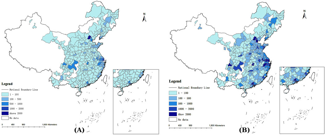
Figure 1. Distribution Maps of Green Patent Counts in Chinese Cities, 2006 (A) vs. 2021 (B).

Given the voluntary nature of environmental disclosure, there is a scarcity of literature directly examining the relationship between environmental technology investment and environmental performance. While most studies affirm a positive correlation between investment in environmental R&D and pollution reduction (Anderson, 2001; Yi et al., 2020), some have revealed nonlinear relationships (Li L. et al., 2021; Li W. et al., 2021). If such nonlinearity exists, advancements in environmental technology may not always yield optimal outcomes. For instance, data from the statistical yearbooks of China’s Ministry of Ecology and Environment show that although capital allocated to environmental protection capacity-building in 2019 increased by 70.1% compared to 2016, pollutant reductions in wastewater and waste gas were largely limited to 13%–18%. This suggests that while investments in environmental technology are crucial, they may encounter diminishing returns at higher levels of investment. Local governments, which are primarily responsible for environmental protection in China, should consider this when allocating subsidies and support for environmental R&D. Failing to do so may result in inefficient use of fiscal resources.

Existing research on the causality between environmental technology and pollution has often relied on methods such as adding higher-order terms to explanatory variables or applying threshold regressions (Du et al., 2019; Luo et al., 2023). However, the Ordinary Least Squares (OLS) approach, with its necessity for predefined model forms, is particularly vulnerable to interference from confounding factors, and it simplistically assumes treatment effects to be constant. The Generalized Random Forests (GRF) method offers a non-parametric alternative that addresses these limitations, moving beyond the constraints of traditional approaches (Athey et al., 2019). This innovative approach autonomously selects covariates to mitigate confounding effects and makes efficient use of covariate information in identifying treatment effects, offering a richer array of statistical features.

This study aims to elucidate the causal relationship between environmental technology R&D investment and pollution reduction. By establishing a social planning problem based on command-and-control environmental regulations, this study first analyzes the mechanisms influencing the emission reduction effects of environmental technologies under equilibrium conditions. Then, using green patent and pollution emission panel data of listed companies across cities in China from 2005 to 2020, it estimates the emission reduction impacts of environmental protection technologies on wastewater, nitrogen oxides, and industrial smoke dust. In addition, besides the traditional OLS method, the study also employs the GRF method to assess the kernel density distribution of the green technology emission reduction effects, and further analyzes the patent categories and city characteristics to identify key factors for formulating targeted pollution emission reduction policies. Therefore, the following three research questions underpin this study.

1. How do environmental technologies affect pollution emissions?

2. What are the differences in the impacts of different categories of environmental technologies on pollution emissions?

3. Which city characteristics can influence the pollution emission reduction effects of environmental technologies?

The potential marginal contributions of this paper can be summarized into three main aspects: First, it analyzes and discusses the issue from the perspective of local governments by constructing a theoretical model aimed at maximizing the welfare of social planners. This theoretical model, yet to be fully discussed, aims to shed light on why solely depending on technological solutions for emissions reduction might not be adequate. Second, it seeks to answer how local environmental regulators can promote the pollution reduction effects of environmental technologies. By examining the heterogeneity in green patent categories and urban characteristics, this study enriches the policy reference contributions of this type of research literature. Third, it enhances the methodological application of causal inference for such problems. The study attempts to use machine learning-based causal inference methods to provide new evidence for the gradually diminishing emission reduction effects of environmental technologies, thereby enriching the details of such treatment effects. Additionally, this paper presents unique findings based on the analysis of emission reduction effects for different pollutants, revealing that due to the varying difficulties in research and development technologies, the convergence speed of their emission reduction effects also varies. A too rapid convergence might render the overall emission reduction effect insignificant.

The remaining contents are organized as follows: Section 2 reviews literature; Section 3 covers theoretical analysis and develops hypotheses; Section 4 details research design and methodology; Section 5 analyzes the treatment effects of green technologies with robustness checks; Section 6 explores patent categories’ heterogeneous impacts; Section 7 re-assesses effects using generalized random forest models and explores factors of variability; Section 8 discusses and Section 9 concludes. See Figure 2 for an overview of the article.

Figure 2

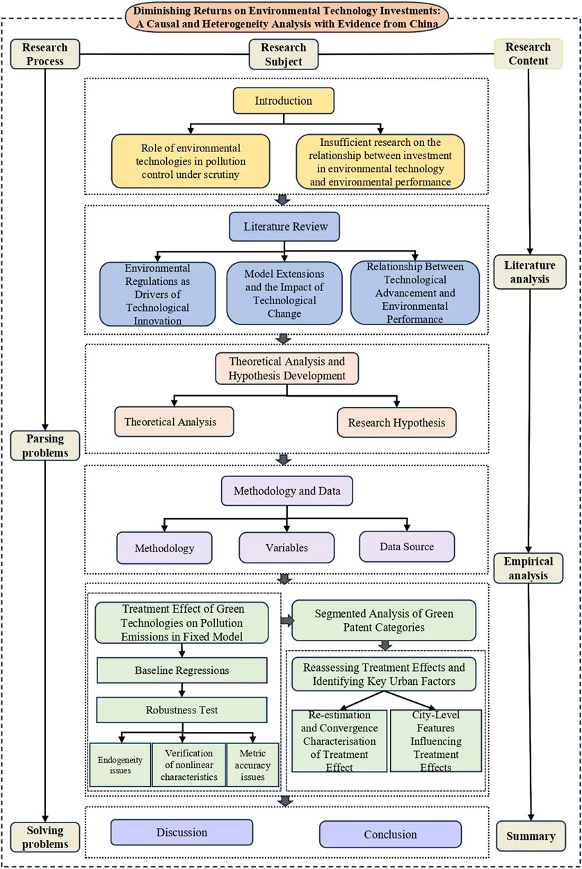
Figure 2. General picture of research.

2 Literature review

In environmental economics, research centered on the Porter Hypothesis predominantly explores the influence of environmental regulations on the progress of sustainable technologies (Barbieri, 2015; Liu et al., 2021). This discourse builds upon Nordhaus’s Dynamic Integrated model of Climate and the Economy (Nordhaus, 1994), with scholars developing and refining models for a greener economy. The model was expanded to embrace learning-by-doing in renewable energy and knowledge spillovers (Otto et al., 2008). In a separate effort, the integration of climate policy-induced technical changes was advocated, supporting subsidies on clean production and pollution taxation to promote environmentally friendly economic development (Acemoglu et al., 2012).

However, does technological advancement in the environmental sector translate into improved environmental performance? This question has been explored in a few studies. On a theoretical level, Induced innovation and learning spillovers were integrated into the model, estimating the energy savings and emission reduction effects of investments in clean technology R&D (Popp, 2010). On the empirical side, research is scarce due to the voluntary nature of corporate environmental information disclosure and the difficulty in distinguishing and measuring investments in environmental R&D at the regional level. Most literature supports a positive linear relationship between environmental R&D and environmental performance. For instance, R&D expenditure was identified as a key factor in reducing Japan’s carbon emissions (Cole et al., 2013), while a positive correlation was found between firms’ R&D investments and the reduction of industrial particulate emissions (Jiang et al., 2014). Some studies assess the effects of technological emission reductions from regional or industrial perspectives, yet their conclusions remain focused on discussions of whether there is a linear correlation (Alam et al., 2019; Carrión-Flores and Innes, 2010; Luo et al., 2023).

Given that the availability of environmental technologies is fixed over a certain period, the returns on investment in these technologies may be nonlinear according to the theory of diminishing marginal productivity (Solow, 1956). Only a few studies have explored this characteristic. Exploring the nonlinear dynamics between environmental R&D investments and environmental performance, an inverse “U-shaped” relationship between R&D expenditure and carbon emission reductions was observed across firms in 52 countries, providing insights into the peak points of marginal effects (Li L. et al., 2021). Similarly, this pattern was also identified within 30 provinces and 32 economic sectors in China, highlighting the complexities of environmental R&D investments’ impact on environmental performance (Li W. et al., 2021). Both studies contribute valuable insights into the discussion of marginal effects’ peak points. However, they gently navigate around the challenge of precisely segregating the fraction of R&D investments dedicated explicitly to environmental objectives, both at the corporate and regional levels.

Furthermore, this topic presents unexplored areas. First, the emission reduction mechanisms of environmental technologies warrant deeper analysis. Current literature, primarily using theories like diminishing marginal productivity, could benefit from integrating economic models for richer insights. Second, technological emission reduction exhibits widespread regional heterogeneity. Although some literature mentions this issue (Costantini et al., 2013; Li et al., 2017), existing studies seldom delve deeply into it. Third, distinguishing investments in environmental technologies more precisely remains a challenge. Studies typically use R&D spending or patent counts as proxies, but these do not specifically pinpoint environmental R&D efforts, highlighting a need for refined causal identification approaches. Lastly, while the nonlinear effects of emission reductions are commonly analyzed through econometric methods, employing machine learning or non-parametric statistics might reveal more detailed findings, though their use in empirical research is less common.

3 Theoretical analysis and hypothesis development

Within a directive environmental policy framework, this study proposes a simple theoretical model to illustrate that environmental or green technology investments may not always yield expected returns. Unlike previous analyses that emphasize market-driven mechanisms (Acemoglu et al., 2012; Aghion et al., 2016), this study considers China’s environmental governance issues as a societal planning problem, wherein the government can directly adjust enterprises’ production scales. Specifically, while Acemoglu et al. (2012) explore the dynamic effects of carbon taxes and research subsidies on innovation direction, and Aghion et al. (2016) focus on the path dependency of technical change in response to fuel prices, this study highlights the unique institutional features of China’s dual-track policy system. Despite China’s piloting of market-based instruments like emissions trading since the 1990s, administrative measures and command-and-control policies have remained predominant in industrial production interventions until 2020 (Tang H. et al., 2020; Tang K. et al., 2020).

In this societal planning issue, total social utility depends on consumption $C$ and pollution emissions $E$. In the current scenario, enterprise labor input remains fixed, and ignoring capital depreciation. In other words, each enterprise’s production function is a function of the capital input $K_i$. Societal pollution emissions result from summing individual enterprise emissions, calculated as one minus the pollution treatment rate function, $g\left(k_i\right)$, multiplied by the product output $Y_i$. Here, $g\left(k_i\right)$ represents the impact of environmental R&D investment $k_i$.

Social planners optimize enterprise production scales to maximize the social utility function $U\left(C,E\right)$, subject to consumption meeting national income equality, and short-term total investment capped at $K_{\mathit{max}}$, with total pollution below $E_{\mathit{max}}$. In essence:

$\underset{K_1,K_2\cdots K_n}{\max }U\left(C,E\right)$

$s.t.\left\{\begin{array}{l}\begin{array}{l}C=\sum Y_i-\sum K_i\\ Y_i=f\left(K_i\right)\\ E=\sum \left[1-g\left(k_i\right)\right]\cdot Y_i,0\le g\left(k_i\right)\le 1,g^{\prime }\left(k_i\right)\ge 0\end{array}\\ k_i={\delta }_i\cdot K_i,0\le {\delta }_i<1\\ \sum K_i=K_{\mathit{max}}\\ \sum E_i\le E_{\mathit{max}}\end{array}\right.$

Typically, the total utility function $U\left(C,E\right)$ is positively correlated with consumption C and negatively correlated with emissions E. $f\left(K_i\right)$ is the production function for enterprise $i$ with respect to capital input $K_i$​. Assuming $g\left(k_i\right)$ is monotonically non-decreasing with environmental R&D investment $k_i$. The proportion of pollution emission reduction caused by a unit increase in environmental investment $k_i$ can be denoted as ${MRE}_i=g^{\prime }\left(k_i\right)$, and $k_i$ can be simplified as a proportion of the total capital input $K_i$ for enterprise $i$, with ${\delta }_i$ reflecting its share.

The above scenario is based on a command-and-control environmental policy framework, where the government can adjust the scale of enterprise production through administrative orders, pollution taxes, and similar measures. With emission rights trading, businesses decide between reducing emissions or buying rights, weighing governance costs against rights acquisition costs. Some studies have examined this issue (Liu et al., 2020; McGartland and Oates, 1985).

It is evident that more output increases social utility, but also generates more pollution, which reduces social utility. To delve deeper into the aforementioned planning problem, it can be assumed that the production function for each enterprise follows the constant returns to scale Cobb-Douglas production function:

$Y_i=A{K}_i^{\alpha }{L}_i^{1-\alpha },0<\alpha <1$

Where the technological level $A$ and labor input $L_i$ can be considered as fixed values in the short term, and $\alpha$ is the output elasticity of capital. The marginal effect of environmental technology investment on total societal pollution emissions is:

$\frac{\partial E}{\partial k}=\sum \left[\left(1-g\left(k_i\right)\right)\frac{\partial Y_i}{\partial k_i}-{MRE}_i\cdot Y_i\right]$

$=\sum \left(\frac{1-g\left(k_i\right)}{{\delta }_i}\cdot \frac{\alpha }{K_i}-{MRE}_i\right)\cdot Y_i=\sum \left(\frac{1-g\left(k_i\right)}{k_i}\cdot \alpha -{MRE}_i\right)\cdot Y_i(1)$

The above equation indicates that whether an increase in the unit environmental investment can reduce total pollution emissions depends on the sum of the marginal effects of environmental investments by each company. In fact, if there is only one enterprise, social planners would have the enterprise invest $K_{\mathit{max}}$ in production, while the enterprise would choose an appropriate $\delta$ to meet the emission limit $E_{\mathit{max}}$. Due to both $MRE$ and $1-g\left(k\right)$ being positive, it must hold that:

$\frac{\partial E}{\partial \delta }=-\left[MRE\cdot k+\left(1-g\left(k\right)\right)\cdot \alpha \right]\cdot \frac{Y}{\delta }<0$

This indicates that as the proportion of environmental investment increases, pollution emissions will correspondingly decrease. However, when the problem involves multiple enterprises, differences in the research and production capabilities of each company introduce uncertainty into the sign of the term within the brackets in Equation 1, making the marginal effect of environmental investment on total societal pollution emissions uncertain. Factors include the functional form of g(k), R&D investment, and output quantity as weights. To further discuss the sufficient conditions for the existence of equilibrium solutions, this paper assumes the utility function to be in its simplest linear form:

$U=C-\beta E$

Where β is the coefficient representing the aversion to pollution per unit of societal consumption, typically assumed to be greater than 0. Alternatively, assuming a Constant Elasticity of Substitution (CES) utility function form also yields similar conclusions. If equilibrium exists, the corresponding first-order condition is:

$\frac{\alpha Y_i}{K_i}=\frac{1-\beta {\delta }_i\cdot {MRE}_i}{1-\beta \left(1-g\left(k_i\right)\right)},or{K}_i=\frac{\left[1-\beta \left(1-g\left(k_i\right)\right)\right]\cdot \alpha Y_i}{1-\beta {\delta }_i\cdot {MRE}_i}$

The above equation indicates that if an equilibrium exists, the marginal output of capital for each company at the equilibrium state should be distributed according to the environmental efficiency ratio based on its utility function. In addition, the existence of equilibrium should also satisfy second-order conditions. Specifically, at the equilibrium point $k_i^{*}$, it should hold that:

$g^{″}\left(k_i^{*}\right)\cdot k_i^{\ast 2}+2\alpha g^{\prime }\left(k_i^{*}\right)k_i^{*}+\alpha \left(\alpha -1\right)g\left(k_i^{*}\right)<0$

$g^{″}\left(k_i^{*}\right)<-\frac{2\alpha g^{\prime }\left(k_i^{*}\right)k_i^{*}+\alpha \left(\alpha -1\right)g\left(k_i^{*}\right)}{k_i^{\ast 2}}$

The right-hand side of above inequality is always non-negative, imposes a crucial requirement: the second derivative of the pollution treatment rate function around $k_i^{*}$​ must be negative. This condition indicates that the environmental R&D efficiency is marginally decreasing near the stable point, which generally aligns with real-world scenarios. Due to the finite stock of basic science behind specific pollutant reductions over a certain period, there are constraints on available technology development. This results in diminishing marginal effects of R&D investment on pollution treatment rates, explaining the nonlinearity of environmental technology’s emission reduction effects. Rational enterprises cease further investment in environmental R&D when the marginal effect diminishes to zero, aligning with our previous assumption of non-negativity for $g^{\prime }\left(k_i\right)$. Therefore, it can be proposed the following research hypothesis:

Research Hypothesis: The marginal effect of environmental R&D investment on pollution reduction is nonlinear, potentially leading to a diminishing actual technological emission reduction effect.

To further assess the economic value of green innovation, we simplify the model to a single firm scenario, where R&D investment $k$ is a fixed proportion $\delta$ of capital input $K$. The marginal benefit of emission reduction (MB) can be expressed as:

${\text{MB}}_{\text{RP}}=\beta A{K}^{\alpha }{g}^{\prime }\left(\delta K\right)\delta$

while the marginal cost of green innovation (MC) is:

${\text{MC}}_{\text{GI}}=1-\alpha A{K}^{\alpha -1}\left(1-\beta +\beta g\left(\delta K\right)\right)$

When ${\text{MB}}_{\text{RP}}<{\text{MC}}_{\text{GI}}$​, further investment in green innovation no longer yields economic benefits. This analysis highlights the importance of balancing the costs and benefits of green innovation in policy design, particularly in determining optimal investment levels to maximize social welfare.

4 Methodology and data

This section outlines the methodologies employed, specific model configurations, variable definitions, and the selection and characteristics of the sample used in the study.

4.1 Methodology

The empirical section aims to examine whether there is a nonlinear emission reduction effect associated with environmental technology R&D investments, with a focus on whether the marginal effects diminish as investments increase. To achieve this objective, this study employs a fixed-effects model augmented with quadratic terms to estimate the treatment effects. Fixed effects absorb unobserved factors, mitigating omitted variable bias for more accurate estimation of treatment effects. The inclusion of quadratic terms for explanatory variables in the model also helps capture potential nonlinear treatment effects. This model specification is inspired by relevant literature (Li L. et al., 2021), and its form is set as follows:

${Emission}_{it}={\beta }_0+{\beta }_1{Patents}_{it}+{\beta }_2{Patents}_{it}^2+{\gamma }_k\sum X_k+{\mu }_{\mathit{i}}+{\tau }_t+{\epsilon }_{it}(2)$

In the above equation, ${Emission}_{it}$ represents the dependent variable, corresponding to the emissions of three types of pollutants in the ith city in the tth year. ${Patents}_{it}$ is the core explanatory variable. In this study, the total count of green patents aggregated at the enterprise level is used as a proxy variable for green technology investment. ${\beta }_1$ signifies the treatment effects of green patents on pollution emissions. ${\beta }_0$ is the intercept term of the regression, $X_k$​ denotes the control variables, and the vector ${\gamma }_k$ represents their respective coefficients. The model controls for individual fixed effects ${\mu }_{\mathit{i}}$ and time fixed effects ${\tau }_t$ . ${\epsilon }_{it}$ is the random error term.

However, linear models based on the aforementioned method, when estimating the effect of the treatment variable W on the outcome variable Y based on control variables X, require a predefined model form, and the treatment effect τ is also assumed to be constant. In this case, confounding factors need to be fixed in advance, hence nonlinear treatment effects might not always eliminate endogenous interference. To address this issue, this paper also re-estimates treatment effects using the generalized random forests (GRF) method (Athey et al., 2019). This approach represents a recent development in machine learning for causal inference, relaxing constraints on model form and the constancy of τ (Rubin, 2005). The GRF model, by estimating the propensity score $e\left(x\right)$ and $m\left(x\right)=E\left[Y_i|X_i=x\right]$, leads to the following central form:

$Y_i-m\left(x\right)=\tau \left(W_i-e\left(x\right)\right)+{\epsilon }_i$

In this formulation, as long as either m(x) or e(x) can be accurately estimated, the conditional treatment effects $\tau \left(X_i\right)=E\left[Y\left(1\right)-Y\left(0\right)|X_i=x\right]$ can be estimated with greater consistency. Moreover, given the forest model’s ability to freely choose covariates, this method can enhance estimation accuracy by providing a larger, dimensionally invariant set of covariates. Unlike traditional linear models that assume a constant treatment effect, the GRF method allows for the estimation of heterogeneous treatment effects across cities, accounting for differences in regulatory frameworks, economic conditions, and technological adoption. Compared to linear models, this non-parametric statistical method can yield the distribution of treatment effects, thereby offering richer statistical information conducive to a deeper exploration of the trends in treatment effects over time.

Leveraging previous foundational work (Breiman, 2001; Robinson, 1988), the algorithm first places the covariate split “greedily” in the spanning tree stage to maximize the squared difference of treatment effects, and then estimates the treatment effects based on the adjusted Equation 2 after building the random forest model. In the model fitting process, GRF assigns importance scores based on the frequency of covariate usage, estimating the optimal linear projection of the treatment effects on a series of the most significant covariates, thereby capturing heterogeneous treatment effects. This feature is beneficial for further contemplating which city characteristics can affect the magnitude of the treatment effects and how they do so, thereby positively influencing policy formulation.

This study employs Stata 16.0 for estimating the fixed effects model, the “grf” package in R for fitting, estimating, and visualizing the GRF model, and Python 3.7’s “jieba” library among others for text analysis.

4.2 Variables

This paper employs various urban-level pollutants as dependent variables, encompassing sewage emission (Emission_sewage), nitrogen oxide emission (Emission_NOx), and industrial smoke and dust emission (Emission_sd). These three pollutants with good data quality at the urban level are selected for their reflection of varying technological challenges in pollution control. Sewage emission control technologies, such as biological and chemical treatments, are the simplest. Nitrogen oxide (NOx) emission reduction techniques, like Selective Catalytic Reduction (SCR) and Selective Non-Catalytic Reduction (SNCR), represent intermediate complexity. Industrial smoke and dust emission mitigation, requiring advanced Electric-Bag Composite Dust Removal, poses the greatest technical challenge.

This study employs aggregated city-level green patent data of listed companies as the primary explanatory variable. Although R&D spending could more closely indicate environmental innovation efforts, the use of green patents is dictated by challenges in obtaining firm-specific pollution data and distinguishing the environmental portion of R&D investments due to voluntary disclosure practices. The patents are classified per the United Nations Framework Convention on Climate Change into six categories: waste management, nuclear power, transportation, energy conservation, alternative energy production, and administrative regulation and design, with the possibility of patents overlapping across categories.

Informed by literature (Du et al., 2019; Du and Li, 2019), this paper selects control variables influencing both pollution emissions and green technology outputs. Key variables include the logarithm of per capita GDP (LnPGDP), treated to approximate growth rates while maintaining variables in a comparable dimension, and the ratio of government R&D investment to GDP (Ratio_rd), addressing technological support’s impact. Foreign direct investment (FDI) and industrial structure (IS) are assessed to gauge polluting enterprises’ prevalence in cities. Additionally, environmental regulation is assessed using Python text analysis on city government work reports, extracting and categorizing relevant Chinese terms. The frequency of these terms is normalized to formulate the Environmental Regulation index (ER), indicating local governments’ focus on environmental concerns, with detailed vocabulary presented in Table 1.

Table 1

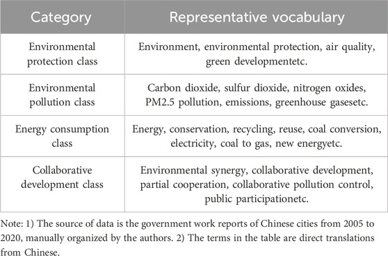
Table 1. Text analysis word frequency statistics of each category name and some representative words.

In the GRF model section, this paper constructs a covariate set with theme-related variables from the China City Statistical Yearbook, including per capita GDP, government research and education spending as ratios to GDP, and broadband subscribers per household registration, etc. Descriptive statistics for the main variables involved are presented in Table 2.

Table 2

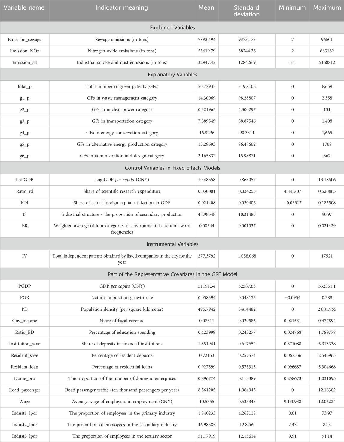
Table 2. List of variables and descriptive statistics.

4.3 Data source

The green patent data used in this paper comes from the China Stock Market Accounting Research Database (CSMAR, https://www.gtarsc.com/). The dataset consists of 173,674 green patent records spanning from 1992 to 2021. Frequency analysis revealed that the data for 2021 significantly fell below the average level of the preceding 3 years. To ensure data accuracy, the 2021 data were excluded. The patent records include the securities code of the involved listed companies, the fiscal year, the company name, the relationship between the company and the relevant listed company, the patent application date and authorization date, and whether the patent is an invention. Since there is a lack of pollution emission data at the enterprise level, the data was aggregated to the city level based on the postal codes of office addresses of the listed companies in the database.

This study’s city-level socio-economic data, sourced from the China City Statistical Yearbook, underwent preprocessing to enhance reliability: Cities with significant data gaps or administrative changes were excluded. Missing patent data were set to zero, and were verified and adjusted using local and provincial yearbooks. Interpolation methods filled remaining gaps, ensuring missing values constituted less than 0.5% of the data, minimizing their impact on analyses. This paper identify outliers as those values exceeding three standard deviations above the mean, and we have applied Winsorization to a minimal number of extreme values to ensure they do not become leverage points in the estimation of treatment effects within linear model. The refined dataset comprises a balanced panel for 217 cities from 2005 to 2020.

5 Treatment effect of green technologies on pollution emissions in fixed model

5.1 Baseline regressions

This paper initially estimates Equation 2, with results presented in Table 3. In columns (1), (3), and (5), the regression estimates include only the quadratic term of the total number of green patents, the variable s_total_p with the prefix “s_” represents the square of the total number of patents. Columns (2), (4), and (6) present the estimates with the inclusion of city-level control variables.

Table 3

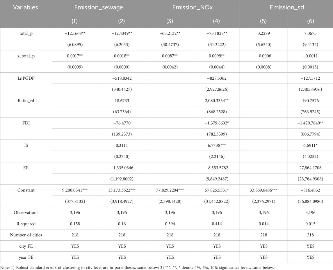
Table 3. Estimated results of baseline regressions.

The estimated results indicate that green patents have a certain emission reduction effect on sewage and nitrogen oxides, which is statistically significant at a 5% significance level. However, the treatment effect on industrial smoke and dust is not statistically significant. For the two pollutants where the treatment effect is significant, the estimated coefficient for the linear term of green patents, i.e., the marginal effect of pollution reduction, is negative. Simultaneously, the quadratic term coefficient is positive, suggesting a diminishing marginal effect on pollution reduction with an increase in the number of green patents.

Using sewage emissions as an example, the marginal effect can be expressed in a linear form: −12.4349 + 0.0018 × number of patents. This indicates that at the initial stages of environmental technology application, each patent contributes to a reduction of approximately 12.43 tons in sewage emissions. However, as the number of patents increases, their marginal effect diminishes, approaching a reduction effect close to zero when the green patent count nears 6,908. The results partially validate the research hypothesis, yet the impact on industrial smoke and dust did not exhibit statistical significance. Subsequent sections aim to explain this phenomenon by examining the nuanced categories of patents and the convergence rate of their marginal effects.

5.2 Robustness test

5.2.1 Endogeneity issues

The potential bidirectional causality between patents and emissions introduces endogeneity issues. This paper adopts strategies from the literature on addressing peer effects (Bentolila et al., 2010; Card and Krueger, 1996) and selects the total number of independent patents obtained by all listed companies in a city within the year as an instrumental variable (IV) for the linear term of patents. This variable is directly related to the city’s green patents but not directly to emissions. Additionally, given the potential endogeneity of the quadratic term, the square of the instrumental variable (IV_sq) is introduced as an additional instrument for the quadratic term of patents. Using the two-stage least squares method, results are presented in Table 4.

Table 4

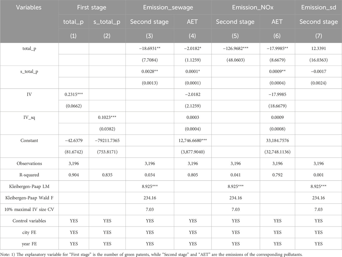
Table 4. Results of instrumental variable estimation of green patents on pollution emissions.

Table 4, Columns (1) and (2), report the first-stage regressions for the linear and quadratic terms of patents, respectively. Column (1) takes the total number of green patents as the dependent variable and uses the original instrumental variable (IV) as the primary explanatory variable. The estimated coefficient of IV passes the 1% significance level test, indicating a strong correlation between IV and the total number of green patents. Similarly, Column (2) uses the square of the total number of green patents as the dependent variable and employs both IV and its square (IV_sq) as explanatory variables. The coefficient of IV_sq is also significant at the 1% level, confirming the relevance of the quadratic instrument.

Columns (3) to (7) present the second-stage and approximate exogeneity test (AET) results for the three pollutants. Columns (3), (5), and (7) show the second-stage regression results for sewage, nitrogen oxide, and industrial smoke and dust emissions, respectively. The second-stage estimations indicate that the marginal abatement effects of green patents on sewage and nitrogen oxide emissions remain significant, with the absolute values of the coefficients increasing compared to the baseline regression. For industrial smoke and dust emissions, however, the abatement effect of green patents remains insignificant.

Columns (4) and (6) provide the results of the approximate exogeneity test (AET) for sewage and nitrogen oxide emissions, respectively. This test involves simultaneously regressing the explanatory variable and the instrumental variables on the dependent variable. The results confirm that the instrumental variables (IV and IV_sq) are exogenous to the dependent variables, as their coefficients become insignificant in this test. This supports the validity of the instrumental variable strategy employed in this study.

5.2.2 Metric accuracy issues

Constrained by the available data, this study is limited to measuring the impact of green technology on pollution emissions at the city level. However, this measurement approach faces three main challenges.

Firstly, the aggregated green patent data’s challenge is their broad indicator, obscuring direct links to specific pollutants, necessitating a refined analysis of patent categories to assess impacts on three pollution types more accurately in later sections. Secondly, focusing solely on patents from listed companies overlooks broader innovation efforts. To rectify this, the study incorporates data from the Chinese Research Data Services Platform (CNRDS, http://www.cnrds.com), encompassing city-specific green patents across all entities. Regression analyses, incorporating this comprehensive variable (GP_citylevel), are detailed in Table 5 (1)–(3), showing consistent trends with the baseline. Thirdly, the geographic specificity of green patent utilization is questioned, as technologies may be applied beyond the originating city’s borders. To ensure accuracy, the study meticulously validated green patent allocations against company locations, adjusting the green patent count (newGP) accordingly. This refined approach, aimed at better aligning patent use with actual company locations, yielded improved estimation accuracy for pollution impacts, as demonstrated in Table 5 (4)–(6), where the results exhibit enhanced coefficients and significance levels for the treatment effects on major pollutants, ensuring the estimation remains robust.

Table 5

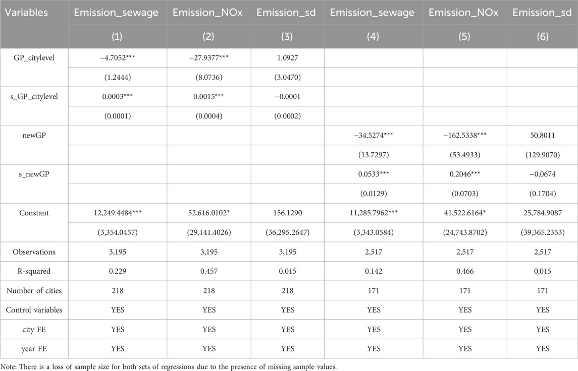
Table 5. Estimates with replacement variables and samples.

5.2.3 Verification of nonlinear characteristics

In the baseline regression, a quadratic term was introduced to capture the nonlinear relationship between green patents and emission reductions. However, this approach may not fully represent the nonlinear dynamics. For example, if the relationship follows an upward-opening parabola, emissions could theoretically increase beyond a certain threshold of green patents, which contradicts practical expectations. To further validate the nonlinear characteristics, this section employs the Bins method, dividing green patents into quintiles and estimating the treatment effects of each group on three pollutants. The results are presented in Table 6, Panel A. Columns (1), (3), and (5) report the effects of group means (Bin_mean) on the three pollutants, consistent with the baseline regression, showing no significant emission reduction effect for industrial smoke and dust. Columns (2), (4), and (6) present the effects of group dummies, with the first quintile (Bin_dummy1) omitted to avoid multicollinearity. The coefficients indicate a diminishing marginal reduction effect for sewage and nitrogen oxides, with emission reductions decreasing as the patent quintiles increase. However, industrial smoke and dust do not exhibit a similar pattern. Notably, the highest quintile shows a relatively strong reduction effect, likely due to stricter emission requirements in densely populated, R&D-intensive cities like Beijing and Shanghai.

Table 6

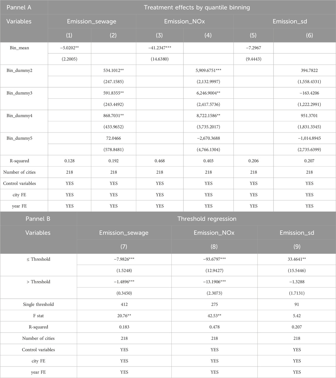
Table 6. Bins grouping regression and threshold regression estimates.

Additionally, threshold regression was applied to re-estimate the baseline model, as shown in Panel B, columns (7)–(9). Sewage and nitrogen oxides exhibit significant single-threshold characteristics, while industrial smoke and dust do not. By examining the coefficients before and after the threshold values (412 patents for sewage and 275 for nitrogen oxides), the reduction effects demonstrate a diminishing trend, gradually approaching zero or a minimal level without reversing.

To further explore these dynamics, this study employs the Quantile-on-Quantile (QQ) regression method (Sim and Zhou, 2015). Green patents and pollutant emissions were divided into 5% quantiles by year, and quantile regressions were conducted for each combination of independent and dependent variable quantiles. The coefficients were averaged across years, and the results are visualized in three-dimensional plots (Figures 3A–C). Darker colors indicate higher reduction effects. The plots reveal a nonlinear pattern where the reduction effect decreases as the number of green patents increases, eventually converging near zero. Industrial smoke and dust (Figure 3C) exhibit a smoother convergence, with a rapid decline around the 40% patent quantile and a post-convergence effect slightly above zero, which may explain its overall insignificance. Additionally, while sewage and industrial smoke and dust show reduced effectiveness in high-pollution quantiles, nitrogen oxides display multiple fluctuations. These findings not only validate the robustness of the baseline regression but also supplement the underfitting of the quadratic model by providing detailed insights into the nonlinear characteristics.

Figure 3

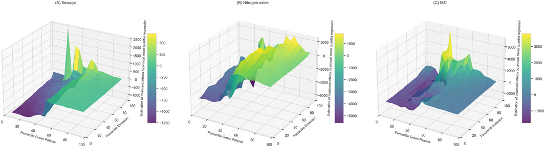
Figure 3. Quantile-on-Quantile (QQ) regression results for green patents’ treatment effects on pollutant emissions. Note: The three-dimensional plots illustrate the relationship between green patent quantiles (x-axis), pollutant emission quantiles (y-axis), and the estimated treatment effects (z-axis) for sewage (A), nitrogen oxides (B), and industrial smoke and dust (C).

6 Segmented analysis of green patent categories

In this section, the paper estimates the emission reduction effects of three pollutants according to six subcategories of green patents. The analysis continues to employ a panel fixed-effects model, incorporating quadratic terms for patents, with the results displayed in Table 7. In Table 7, panel A–C represents three types of pollutant emissions as explanatory variables, and columns 1–6 represent the different categories with the patents as explanatory variables.

Table 7

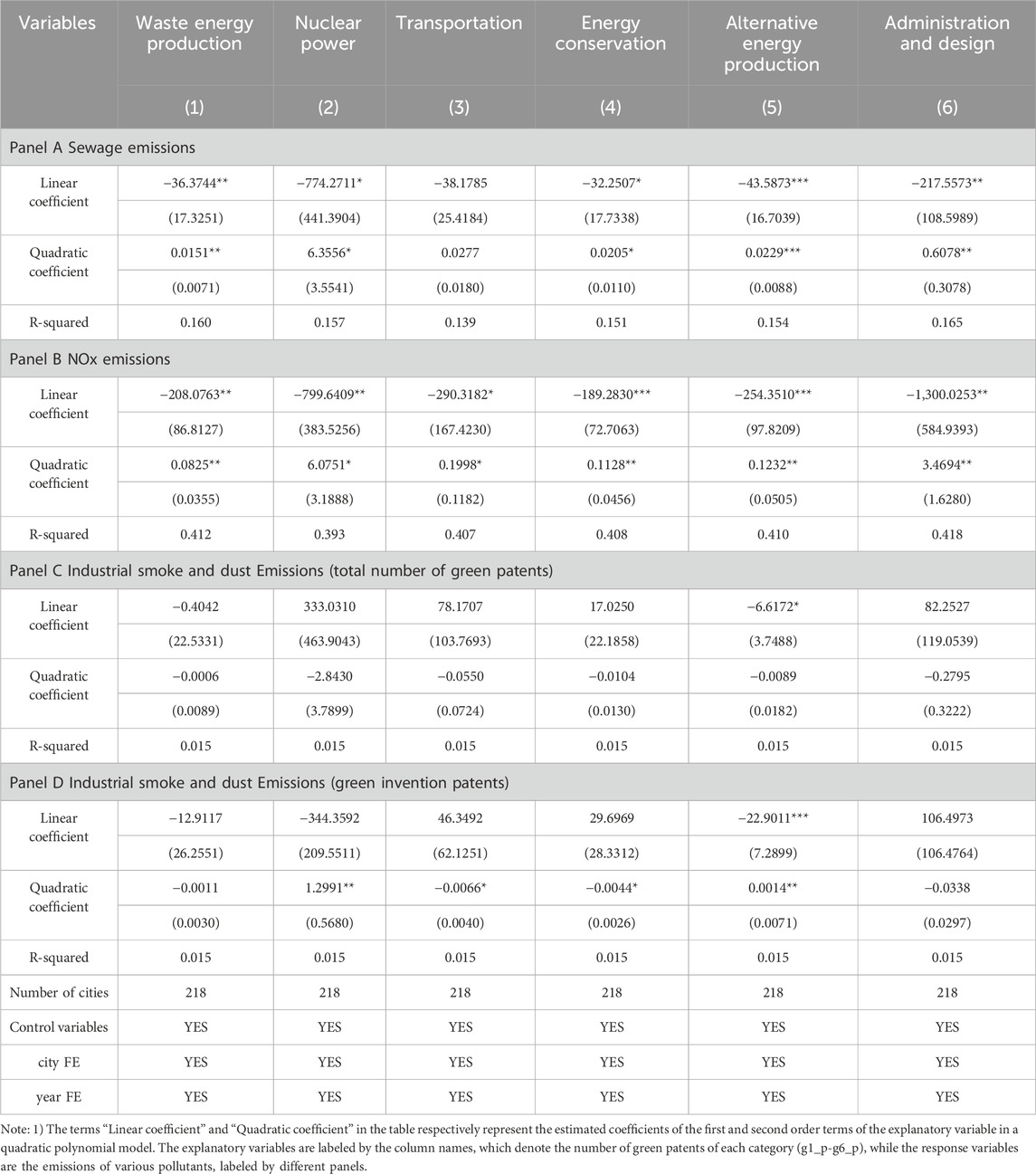
Table 7. Estimates of six categories of green patents on emissions of three types of pollutants.

Panels A and B report the estimated impacts of various patent categories on sewage and nitrogen oxide emissions, respectively, revealing certain similarities. Notably, patents in the nuclear power and administration and design categories exhibit relatively large absolute values for the linear term coefficients, with some significance. This suggests a higher initial emission reduction effect for these two patent types. The study also examines the quadratic term coefficients, which relate to the rate of marginal effect decline. Peak patent numbers for sewage and nitrogen oxide in these categories are similarly close, with nuclear power patents diminishing to zero marginal abatement effect at 122 and 132 patents, and administration and design at 358 and 375 patents, respectively. Particularly, the administration and design category shows a very high intercept for nitrogen oxide emissions, at −1,300.0253 tons, indicating that regulatory technologies are highly effective in early-stage pollution control for this pollutant.

Panel C presents the estimation results for industrial smoke and dust emissions, which, similar to the baseline regression, do not show sufficient statistical significance. The paper then re-estimates these effects using the quantities of invention patents across six categories, with findings reported in Panel D. Uniquely, the linear and quadratic coefficients of invention patents in the alternative energy production category demonstrate 5% significance. According to this analysis, the patent count at which marginal abatement effect declines to zero is 16,358. This outcome suggests that high-quality alternative production technologies might be an effective means to reduce industrial smoke and dust emissions.

7 Reassessing treatment effects and identifying key urban factors

In this section, a Generalized Random Forest (GRF) model is employed to reevaluate the treatment effects of green patents. Additionally, we identify key urban factors influencing these treatment effects by leveraging the frequency with which covariates are used in constructing the model.

The algorithm initiates by estimating propensity scores ($\widehat{\mathit{W}}$) and conditional expectations ($\widehat{\mathit{Y}}$), utilizing selected dependent, treatment variables, and a covariate set, with the aim of enhancing the robustness and accuracy of causal effect estimations. This involves two key hyperparameters critical to the model’s optimization: parameter 1, which sets the covariate significance threshold for model inclusion, and parameter 2, determining the causal forest model’s number of trees. These parameters are pivotal, with parameter one varying from 0 to 0.5 in increments of 0.05, and parameter two spanning from 100 to 1,500 trees in steps of 100, to systematically explore the parameter space for the optimal model configuration. This exploration aims to identify the settings that yield the highest model fit, culminating in the estimation of the average treatment effect (ATE) based on the optimally configured causal forest model.

7.1 Re-estimation and convergence characterisation of treatment effect

Following the outlined process to identify the optimal GRF models for various pollutants, this paper employs the optimal model to estimate the kernel density distribution of the treatment effects of green patents. The GRF model not only estimates the average treatment effects of green patents but also reveals how these effects evolve over time and across regions. This dynamic perspective is crucial for understanding the long-term impacts of emission reduction policies, highlighting the diminishing returns of green patents in some contexts and the persistence of high-impact effects in others. Such insights are pivotal for tailoring policy interventions to regional characteristics. In the estimation strategy, cities are used as clustering units to ensure that random sample division can be organized by city. Additionally, the study divides the sample into different time intervals to observe whether the marginal abatement effects decrease over time, as hypothesized.

Table 8 reports the model fitting outcomes and average treatment effect estimates for the quantity of green patents concerning three pollutants, where the sample is divided into three time periods: 2005–2010, 2011–2015, and 2016–2020. The fourth column of the table reports the overall estimates for the period 2005–2020. Where the MFP (mean forest prediction) indicator tests the superiority of model fit, and the closer the indicator is to 1, the better the model fit. The DFI (differential forest prediction) indicator verifies whether the model has heterogeneity characteristics regarding covariates, and ATE (average treatment effect) reports the results of the average treatment effect.

Table 8

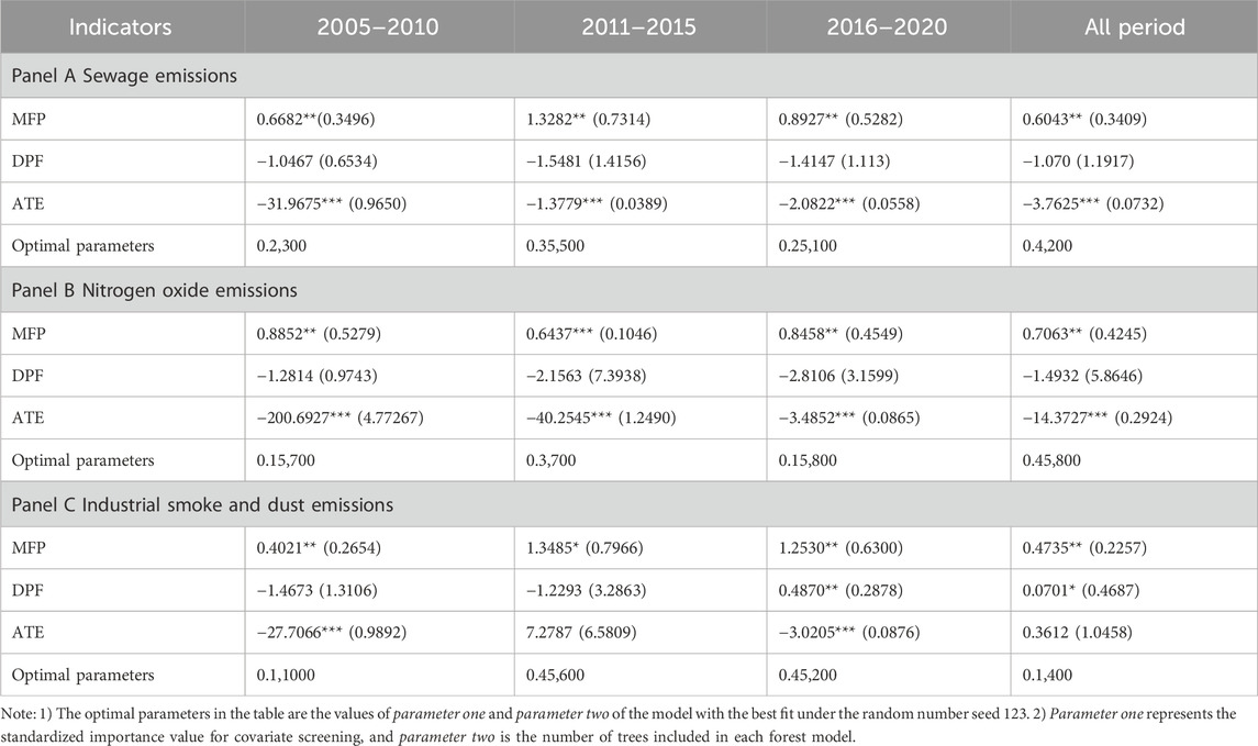
Table 8. GRF model fitting and average treatment effect estimation for green patents on three types of pollutants.

Panels A–C of Table 8 respectively present the model fitting outcomes and treatment effect estimates of green patents for sewage, nitrogen oxide, and industrial smoke and dust. The model fittings under the optimal parameter settings exhibit statistically significant results, indicating a good fit for the models.

Table 8’s “All period” spans 2005–2020, matching the fixed effects model’s timeframe. Re-estimating green patents’ ATE on pollutant emissions, the GRF model found significant effects for sewage and nitrogen oxide, but not for industrial smoke and dust, with ATEs of −3.7625, −14.3727, and 0.3612 tons, respectively. Comparatively, the fixed effects model, with its intercepts and slopes, is not directly comparable to the GRF model. Yet, treating the GRF model’s 2005–2010 ATEs as the fixed model’s baseline (intercepts can be regard as initial ATEs), GRF estimates (−31.968, −200.693, −27.707 tons) surpass fixed model’s intercepts (−12.435, −73.183, 7.068 tons) in magnitude and significance at 1%.

The findings suggest that green patent technologies initially exhibit a favorable ATE, but their marginal returns may diminish over time, a hypothesis this study aims to test. This paper illustrated the distribution of the treatment effects of green patents on three types of pollutants over time through the kernel density in Figures 4–6 observing similar results.

Figure 4

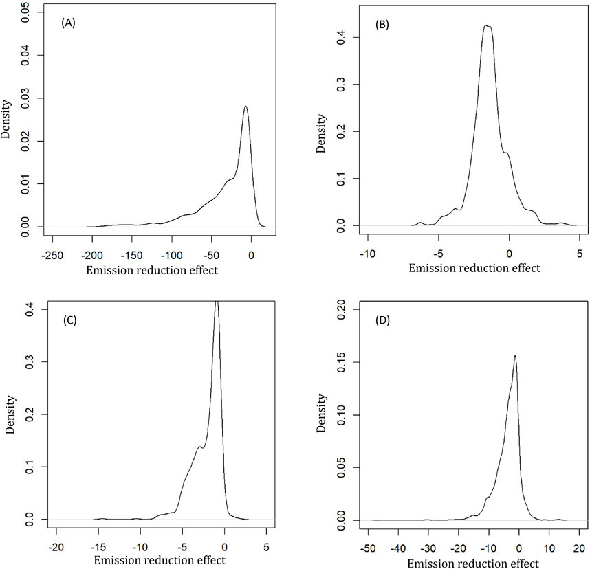
Figure 4. Kernel density distributions for green patents’ treatment effects on Sewage emissions. Note: the distributions are displayed for 2005–2010 (A), 2011–2015 (B), 2016–2020 (C), and the entire time span (D), aligned with the baseline regression timeframe.

Figure 5

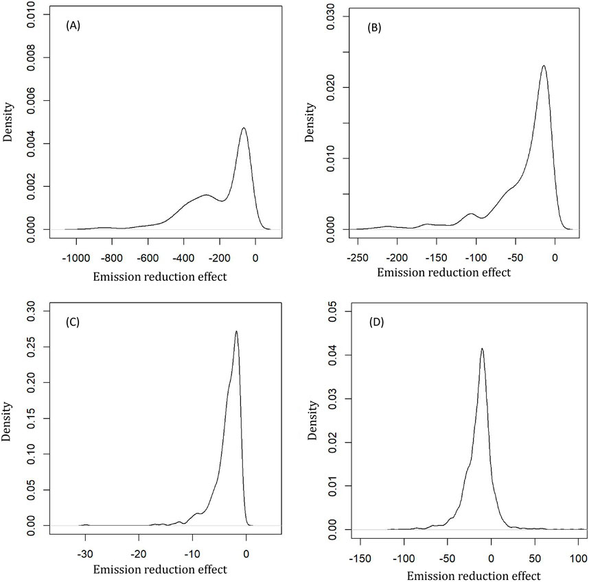
Figure 5. Kernel density distributions for green patents’ treatment effects on Nitrogen oxide emissions. Note: the distributions are displayed for 2005–2010 (A), 2011–2015 (B), 2016–2020 (C), and the entire time span (D), aligned with the baseline regression timeframe.

Figure 6

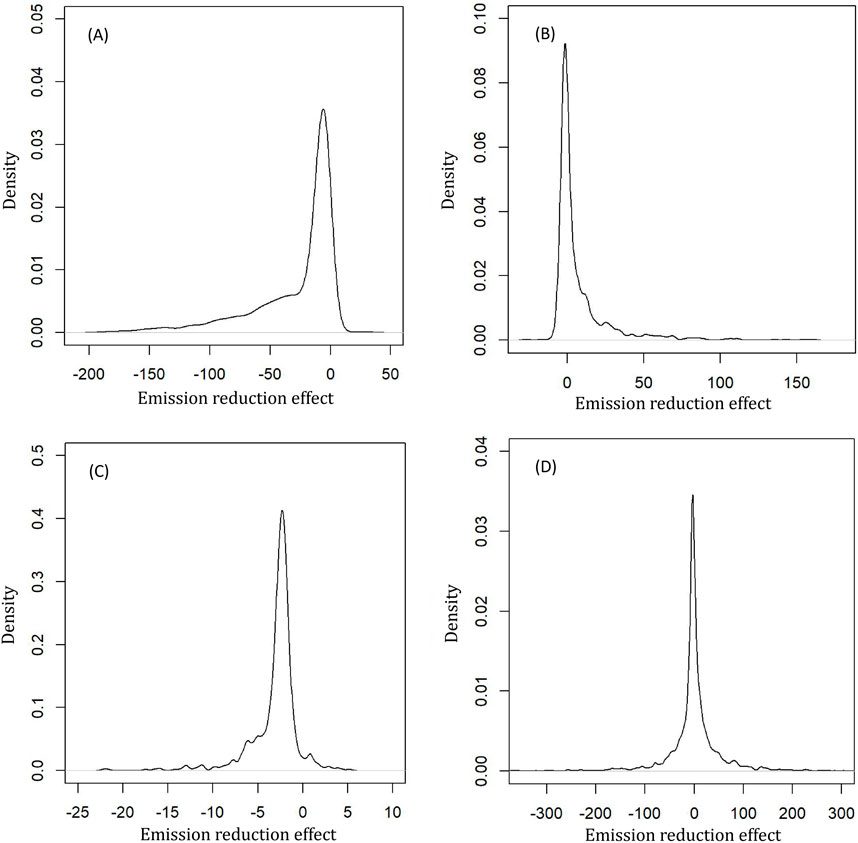
Figure 6. Kernel density distributions for green patents’ treatment effects on Industrial smoke and dust emissions. Note: the distributions are displayed for 2005–2010 (A), 2011–2015 (B), 2016–2020 (C), and the entire time span (D), aligned with the baseline regression timeframe.

Key insights include.

(1) Green patents’ average effects on pollutants decrease over time, with varying speeds of convergence. The 2005–2010 period showed higher average reduction effects for all pollutants (Figures 4–5A), but sewage and industrial smoke and dust emissions nearly converged in the next period (Figure 4B, Figure 6B). Sewage saw a subsequent increase (Figure 4C), possibly from technological breakthroughs, with limited impact on industrial smoke and dust emissions (Figures 5C, 6C).

(2) All categories showed a “long tail” in their kernel density, possibly due to the challenge of precisely identifying whether green patents were utilized for specific pollutant control. Left-skewed tails suggest some reduction in emissions, as with sewage and nitrogen oxides, while right-skewed tails indicate general ineffectiveness in pollution reduction (Figure 6B).

(3) The dispersion trend in the treatment effect densities decreases, with the y-axis scale and kurtosis coefficient increasing over time. This suggests a reduction in effective emission reduction technologies, as average effects gradually converge to zero. For instance, the kurtosis coefficient for industrial smoke and dust emissions increased from 3.1 in 2005–2010 (Figure 6A) to 11.6 in 2016–2020 (Figure 6C).

7.2 City-level features influencing treatment effects

In constructing a GRF model, each covariate is assigned a score reflecting its frequency of use in the nodes of spanning trees. The Best Linear Projection (BLP) is then utilized to estimate the linear influence of covariates on the treatment effect $\tau \left(x\right)$. This study separately estimated the top 10 covariates for three pollutants using models from 2005 to 2020. Covariate rankings were determined by node-splitting importance for each pollutant, scoring from 10 (highest) to 1 (lowest), with an overall score aggregated from all three pollutants. Results are in Table 9.

Table 9

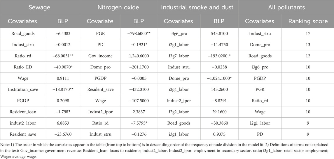
Table 9. Best Linear Projection (BLP) estimation and importance ranking of treatment effects of green patents for three pollutants.

This study organizes covariates into two main categories: Intrinsic Factors and External Support. Intrinsic Factors combine objective conditions and development pressures, capturing the city’s foundational attributes such as industrial structure index (Indust_stru), share of domestic enterprises (Dome_pro), and employment in key sectors (i2g2_labor for manufacturing, i2g1_labor for mining), alongside development challenges like population growth rate (PGR), per capita GDP (PGDP), and real estate sector metrics (i3g6_pro). These variables reflect the economic, industrial, and demographic fundamentals driving environmental policy outcomes.

External Support groups together technology and financial support variables, focusing on the facilitation of green technology through government R&D initiatives (Ratio_rd for R&D expenditure, i3g7_labor for R&D personnel) and education (Ratio_ED for education expenditure), as well as financial resources available for environmental efforts (Institution_save for financial institution deposits, Resident_save for resident savings). This classification highlights the pivotal role of government policy, research and development, and financial mechanisms in supporting the adoption and effectiveness of green technologies and initiatives.

Table 9 reveals key factors affecting green patents’ treatment effects on three pollutants: sewage, nitrogen oxide, and industrial smoke and dust. For sewage, government R&D investment (Ratio_rd) and financial institutions’ deposits (Institution_save) are pivotal, as they directly enhance cities’ capacities to adopt and implement green technologies. For nitrogen oxide, population growth and density (PD) play significant roles by facilitating technology spillovers in more densely populated areas, while government R&D support (Ratio_rd) further amplifies these effects. For industrial smoke and dust, employment in specific industries like real estate (i3g6_pro) and construction (i2g4_labor) reduces the effectiveness of green patents, suggesting that cities with higher proportions of industrial workers may require tailored policy interventions to offset these challenges.

Government support for R&D emerges as a critical external factor across all pollutants, highlighting its importance in enhancing the effectiveness of green patents in emission reduction. The heterogeneous analysis further reveals that cities with higher R&D investment and education expenditure tend to benefit more from green technologies. This implies that national and local governments should prioritize funding for regions with strong technological infrastructure while offering targeted support to less-developed areas to bridge the gap in technological adoption and effectiveness.

8 Discussion

Unlike much of the literature based on endogenous growth models, this article frames the discussion of the relationship between environmental R&D and pollution reduction within a social planning issue, examining the factors that influence the marginal effects of technological emission reduction under command-and-control environmental regulations. It finds that the difficulty of R&D is a pivotal factor, and the existence of an equilibrium solution implies bottlenecks in technological development, highlighting that overcoming these bottlenecks in environmental technology is key to avoiding this predicament.

This study confirms the nonlinear relationship between environmental technology and pollution reduction through a panel fixed effects linear regression model, aligning with conclusions from some existing research (Li L. et al., 2021; Li W. et al., 2021). However, unlike (Li L. et al., 2021), which focuses on the strategies of firms at the turning point of R&D investment, this paper provides new evidence through a re-estimation of the treatment effect kernel density using the GRF model. It suggests that the presence of a turning point is not fixed; there is still potential for marginal emission reduction effects to increase with the advancement of new technologies. Nevertheless, the common trend is that the marginal benefits of technological emission reductions gradually converge to zero, with the rate primarily dependent on the difficulty of R&D.

The treatment effect estimates for green patent subcategories show that nuclear and administrative patents have larger first-order coefficient absolute values compared to other subcategories, indicating a favorable emission reduction effect in the early stages of technology application. These first-order coefficients, or intercept terms of marginal effects, represent the treatment effects before diminishing returns begin. A larger absolute value suggests a more significant initial emission reduction effect, especially for countries just starting technological emission reduction. Unlike nuclear technology, administrative patents, such as pollution monitoring technologies, have lower technical barriers and wider applicability, aligning with existing literature conclusions (Jiang et al., 2014).

Identifying urban characteristics and optimal linear projection results, urban development pressures emerge as the primary factors influencing the effectiveness of green patents in emissions reduction. Local officials in China face dual pressures from urban economic development and environmental performance assessments. These include factors like industrial structure, population, and economic growth, with population growth rate (PRG) showing a heterogeneous treatment effect on the reduction of nitrogen oxides—cities with higher PRGs achieve greater emissions reductions. Our analysis of urban characteristics underscores the importance of tailoring environmental policies to local conditions. For instance, cities with higher population growth rates may achieve greater reductions in nitrogen oxide emissions through green technologies, suggesting that policymakers should consider demographic trends when allocating resources. Furthermore, government expenditure on education and R&D, as well as financial market support, play critical roles in enhancing the effectiveness of green patents. Policymakers should leverage these insights by increasing investments in education and R&D, while also fostering financial mechanisms that support environmental innovation.

The study also highlights two other critical factors: the government’s expenditure ratio on education and R&D, and the capital stock in financial markets, underscoring the importance of policy support and financial investment in R&D outcomes. This finding differs from Li et al. (2017), which identified technology adoption as the primary heterogeneous factor (Costantini et al., 2013; Li et al., 2017). Furthermore, our cost-benefit analysis highlights the importance of balancing the marginal benefits of emission reduction against the marginal costs of green innovation, offering policymakers a critical framework for optimizing resource allocation in environmental technology investments.

9 Conclusion

This paper constructs a planning problem aimed at maximizing social utility under command-and-control environmental regulations and analyzes the impact mechanism of technological emission reductions. By discussing the difficulty of technology under equilibrium conditions, it posits a research hypothesis on the nonlinear marginal effects of environmental technology. The hypothesis is tested through an estimation of the emission reduction effects of green patents held by Chinese listed companies from 2005 to 2020 on three types of pollutants in various cities, using linear regression and Generalized Random Forest models. The analysis further incorporates the heterogeneity of treatment effects across patent categories and city characteristics, offering policy insights.

The findings of this study highlight the diminishing marginal returns of green patents, suggesting that policymakers should adopt a more strategic approach to environmental technology investment. Specifically, local governments should prioritize subsidies for technologies with significant early-stage emission reductions, such as those in nuclear power and administrative design categories. Additionally, increased R&D support is needed for technologies targeting more challenging pollutants, such as industrial smoke and dust, to overcome existing bottlenecks. By aligning fiscal resources with the marginal effectiveness of green technologies, policymakers can maximize the environmental benefits of their investments. Additionally, the preliminary cost-benefit analysis underscores the need for policymakers to carefully evaluate the economic value of green innovation, ensuring that investments yield maximum social and environmental returns.

However, the identification of treatment effects is limited by the scarcity of firm-level emission data, necessitating further refinement for a more precise assessment of the impact of environmental technologies. For this study, potential sources of statistical uncertainty in our estimates may include biases in data recording, the possibility of omitted variable bias, underfitting in the linear model, and inaccuracies in the pre-estimated parameters of the GRF model. Additionally, the theoretical analysis, rooted in a centralized planning context, suggests the need for further exploration into how technological emission reductions perform under diverse environmental regulatory frameworks, such as decentralized economies with market-based instruments like emission trading or pollution taxes. Such comparisons could provide a more comprehensive understanding of the effectiveness of environmental technologies across different governance structures.

Data availability statement

Publicly available datasets were analyzed in this study. This data can be found here: https://data.csmar.com/, http://www.cnrds.com.

Author contributions

XY: Methodology, Software, Writing–original draft. BX: Data curation, Writing–review and editing. JL: Supervision, Writing–review and editing. JW: Writing–review and editing.

Funding

The author(s) declare that financial support was received for the research, authorship, and/or publication of this article. This study was funded by the Jinan Office of Philosophy and Social Science, China (Project No. JNSK23C63), under the leadership of Jia Li.

Acknowledgments

The authors thank the reviewers for their help in improving the quality of this paper.

Conflict of interest

The authors declare that the research was conducted in the absence of any commercial or financial relationships that could be construed as a potential conflict of interest.

Generative AI statement

The author(s) declare that no Generative AI was used in the creation of this manuscript.

Publisher’s note

All claims expressed in this article are solely those of the authors and do not necessarily represent those of their affiliated organizations, or those of the publisher, the editors and the reviewers. Any product that may be evaluated in this article, or claim that may be made by its manufacturer, is not guaranteed or endorsed by the publisher.

References

Acemoglu, D., Aghion, P., Bursztyn, L., and Hemous, D. (2012). The environment and directed technical change. Am. Econ. Rev. 102, 131–166. doi:10.1257/aer.102.1.131

PubMed Abstract | CrossRef Full Text | Google Scholar

Aghion, P., Dechezleprêtre, A., Hémous, D., Martin, R., and Van Reenen, J. (2016). Carbon taxes, path dependency, and directed technical change: evidence from the auto industry. J. Polit. Econ. 124, 1–51. doi:10.1086/684581

CrossRef Full Text | Google Scholar

Alam, M. S., Atif, M., Chien-Chi, C., and Soytaş, U. (2019). Does corporate r&d investment affect firm environmental performance? Evidence from g-6 countries. Energy Econ. 78, 401–411. doi:10.1016/j.eneco.2018.11.031

CrossRef Full Text | Google Scholar

Anderson, D. (2001). Technical progress and pollution abatement: an economic view of selected technologies and practices. Environ. Dev. Econ. 6, 283–311. doi:10.1017/S1355770X01000171

CrossRef Full Text | Google Scholar

Athey, S., Tibshirani, J., and Wager, S. (2019). Generalized random forests. Ann. Statistics 47, 1148–1178. doi:10.1214/18-AOS1709

CrossRef Full Text | Google Scholar

Barbieri, N. (2015). Investigating the impacts of technological position and european environmental regulation on green automotive patent activity. Ecol. Econ. 117, 140–152. doi:10.1016/j.ecolecon.2015.06.017

CrossRef Full Text | Google Scholar

Bentolila, S., Michelacci, C., and Suarez, J. (2010). Social contacts and occupational choice. Economica 77, 20–45. doi:10.1111/j.1468-0335.2008.00717.x

CrossRef Full Text | Google Scholar

Breiman, L. (2001). Random forests. Mach. Learn 45, 5–32. doi:10.1023/A:1010933404324

CrossRef Full Text | Google Scholar

Card, D., and Krueger, A. B. (1996). School resources and student outcomes: an overview of the literature and new evidence from north and South Carolina. J. Econ. Perspect. 10, 31–50. doi:10.1257/jep.10.4.31

CrossRef Full Text | Google Scholar

Carrión-Flores, C. E., and Innes, R. (2010). Environmental innovation and environmental performance. J. Environ. Econ. Manage 59, 27–42. doi:10.1016/j.jeem.2009.05.003

CrossRef Full Text | Google Scholar

Cole, M. A., Elliott, R. J. R., Okubo, T., and Zhou, Y. (2013). The carbon dioxide emissions of firms: a spatial analysis. J. Environ. Econ. Manage 65, 290–309. doi:10.1016/j.jeem.2012.07.002

CrossRef Full Text | Google Scholar

Costantini, V., Mazzanti, M., and Montini, A. (2013). Environmental performance, innovation and spillovers. Evidence from a regional namea. Ecol. Econ. 89, 101–114. doi:10.1016/j.ecolecon.2013.01.026

CrossRef Full Text | Google Scholar

Du, K., and Li, J. (2019). Towards a green world: how do green technology innovations affect total-factor carbon productivity. Energy Policy 131, 240–250. doi:10.1016/j.enpol.2019.04.033

CrossRef Full Text | Google Scholar

Du, K., Li, P., and Yan, Z. (2019). Do green technology innovations contribute to carbon dioxide emission reduction? Empirical evidence from patent data. Technol. Forecast Soc. Change 146, 297–303. doi:10.1016/j.techfore.2019.06.010

CrossRef Full Text | Google Scholar

Fujii, H., and Managi, S. (2019). Decomposition analysis of sustainable green technology inventions in China. Technol. Forecast Soc. Change 139, 10–16. doi:10.1016/j.techfore.2018.11.013

CrossRef Full Text | Google Scholar

Jiang, L., Lin, C., and Lin, P. (2014). The determinants of pollution levels: firm-level evidence from Chinese manufacturing. J. Comp. Econ. 42, 118–142. doi:10.1016/j.jce.2013.07.007

CrossRef Full Text | Google Scholar

Li, L., McMurray, A., Li, X., Gao, Y., and Xue, J. (2021a). The diminishing marginal effect of r&d input and carbon emission mitigation. J. Clean. Prod. 282, 124423. doi:10.1016/j.jclepro.2020.124423

CrossRef Full Text | Google Scholar

Li, W., Elheddad, M., and Doytch, N. (2021b). The impact of innovation on environmental quality: evidence for the non-linear relationship of patents and co2 emissions in China. J. Environ. Manage 292, 112781. doi:10.1016/j.jenvman.2021.112781

PubMed Abstract | CrossRef Full Text | Google Scholar

Li, W., Zhao, T., Wang, Y., and Guo, F. (2017). Investigating the learning effects of technological advancement on co 2 emissions: a regional analysis in China. Nat. Hazards (Dordr) 88, 1211–1227. doi:10.1007/s11069-017-2915-2

CrossRef Full Text | Google Scholar

Liu, H., Owens, K. A., Yang, K., and Zhang, C. (2020). Pollution abatement costs and technical changes under different environmental regulations. China Econ. Rev. 62, 101497. doi:10.1016/j.chieco.2020.101497

CrossRef Full Text | Google Scholar

Liu, Y., Wang, A., and Wu, Y. (2021). Environmental regulation and green innovation: evidence from China’s new environmental protection law. J. Clean. Prod. 297, 126698. doi:10.1016/j.jclepro.2021.126698

CrossRef Full Text | Google Scholar

Luo, Y., Wang, Q., Long, X., Yan, Z., Salman, M., and Wu, C. (2023). Green innovation and so2 emissions: dynamic threshold effect of human capital. Bus. Strategy Environ. 32, 499–515. doi:10.1002/bse.3157

CrossRef Full Text | Google Scholar

McGartland, A. M., and Oates, W. E. (1985). Marketable permits for the prevention of environmental deterioration. J. Environ. Econ. Manage. 12, 207–228. doi:10.1016/0095-0696(85)90031-2

CrossRef Full Text | Google Scholar

Nordhaus, W. D. (1994). Managing the global commons: the economics of climate change. Cambridge, MA: MIT press.

Google Scholar

Otto, V. M., Löschel, A., and Reilly, J. (2008). Directed technical change and differentiation of climate policy. Energy Econ. 30, 2855–2878. doi:10.1016/j.eneco.2008.03.005

CrossRef Full Text | Google Scholar

Popp, D. (2010). Innovation and climate policy. Annu. Rev. Resour. Econ. 2, 275–298. doi:10.1146/annurev.resource.012809.103929

CrossRef Full Text | Google Scholar

Robinson, P. M. (1988). Root-n-consistent semiparametric regression. Econ. J. Econ. Soc. 56, 931–954. doi:10.2307/1912705

CrossRef Full Text | Google Scholar

Rubin, D. B. (2005). Causal inference using potential outcomes: design, modeling, decisions. J. Am. Stat. Assoc. 100, 322–331. doi:10.1198/016214504000001880

CrossRef Full Text | Google Scholar

Shen, F., Liu, B., Luo, F., Wu, C., Chen, H., and Wei, W. (2021). The effect of economic growth target constraints on green technology innovation. J. Environ. Manage 292, 112765. doi:10.1016/j.jenvman.2021.112765

PubMed Abstract | CrossRef Full Text | Google Scholar

Sim, N., and Zhou, H. (2015). Oil prices, us stock return, and the dependence between their quantiles. J. Bank. Financ. 55, 1–8. doi:10.1016/j.jbankfin.2015.01.013

CrossRef Full Text | Google Scholar

Solow, R. M. (1956). A contribution to the theory of economic growth. Q. J. Econ. Q. J. Econ. 70, 65–94. doi:10.2307/1884513

CrossRef Full Text | Google Scholar

Tang, H., Liu, J., and Wu, J. (2020a). The impact of command-and-control environmental regulation on enterprise total factor productivity: a quasi-natural experiment based on China’s “two control zone” policy. J. Clean. Prod. 254, 120011. doi:10.1016/j.jclepro.2020.120011

CrossRef Full Text | Google Scholar

Tang, K., Qiu, Y., and Zhou, D. (2020b). Does command-and-control regulation promote green innovation performance? Evidence from China's industrial enterprises. Sci. Total Environ. 712, 136362. doi:10.1016/j.scitotenv.2019.136362

PubMed Abstract | CrossRef Full Text | Google Scholar

Yi, M., Wang, Y., Sheng, M., Sharp, B., and Zhang, Y. (2020). Effects of heterogeneous technological progress on haze pollution: evidence from China. Ecol. Econ. 169, 106533. doi:10.1016/j.ecolecon.2019.106533

CrossRef Full Text | Google Scholar

Yin, L., and Wu, C. (2022). Promotion incentives and air pollution: from the political promotion tournament to the environment tournament. J. Environ. Manage 317, 115491. doi:10.1016/j.jenvman.2022.115491

PubMed Abstract | CrossRef Full Text | Google Scholar