Snow parameter retrieval (SPR) algorithm for the GCOM-C/SGLI sensor: validation over the Greenland ice sheet

This paper presents a new snow parameter retrieval (SPR) algorithm for the Global Change Observation Mission-Climate/Second Generation Global Imager (GCOM-C/SGLI) instrument (2018-present). This algorithm combines accurate radiative transfer model (RTM) simulations and Scientific Machine Learning (SciML) methods, Multi-Layer Neural-Network (MLNN) techniques in particular. It provides pixel-by-pixel optically equivalent snow grain size in two layers (i.e., a thin surface snow layer and a deep snow layer), snow impurity concentration and broadband blue- and black-sky albedo which constitute standard SGLI products. In addition, this RTM-SciML algorithm retrieves aerosol optical depth and provides an important retrieval error quality flag. This retrieval error flag, established by comparing reflectances obtained from RTM simulations using the retrieved snow and aerosol parameters as input with the measured reflectances, provides a pixel-by-pixel quality check of the retrieval parameters. Application of the RTM-SciML algorithm to SGLI images obtained over the Greenland Ice Sheet revealed a significant change in snow parameters from a cold July 2018 to a warm July 2019. The inferred blue-sky albedo was in general agreement with field measurements with RMSE = 0.0517 and MAPE = 4.64% for shortwave albedo at the SIGMA-A site, and the black-sky albedo, inferred from retrieved snow parameters, was found to be similar (within 5% relative difference) to the blue-sky values. Although developed specifically for application to data obtained by the SGLI imager, the SPR algorithm can easily be adapted for application to other similar multi-spectral sensors, such as MODIS (already done), VIIRS, and OLCI.

1 Introduction

Long-term global mapping of snow albedo and snow property parameters plays an important role in monitoring of the Earth climate system. Satellite remote sensing has offered a very valuable and powerful way to record the evolution of global snow extent and properties with high temporal and spatial resolution (Frei et al., 2012; Deltz et al., 2012; Tedesco, 2015). The visible and near infrared bands can be used to obtain snow coverage, broadband albedo, and snow physical parameters (Stamnes et al., 2007; Lyapustin et al., 2009b; Zege et al., 2011; Kokhanovsky et al., 2019). In particular, the retrieval of snow physical parameters provides a direct way to determine the spectral albedo and the snow surface radiation budget.

Remote sensing algorithms for snow and ice physical properties have been developed for different satellite sensors, such as the GLobal Imager (GLI) (Stamnes et al., 2007), the Moderate resolution imaging spectroradiometer (MODIS) (Lyapustin et al., 2009b; Painter et al., 2009; Zege et al., 2011), and the Ocean and Land Colour Instrument (OLCI) (Kokhanovsky et al., 2019). Some of these algorithms (Stamnes et al., 2007; Lyapustin et al., 2009b) were based on radiative transfer (RT) model generated lookup tables (LUTs), while others (Kokhanovsky et al., 2019; Zege et al., 2011) were based on analytical methods. A physically based, multiple endmember spectral mixture method (Painter et al., 2009) has also been applied to land surfaces consisting of a mixture of snow, vegetation, rocks, and soil. Sirguey et al. (2009) developed a comprehensive atmospheric correction and inversion scheme to retrieve snow parameters in mountainous areas. More recently, Bair et al. (2021) attempted to retrieve snow impurity concentration under complex sub-pixel mixing conditions using a generalized multispectral unmixing approach. However, these previous methods did not solve the radiative transfer equation for a coupled atmosphere-snow system with multiple layers in the atmosphere and a two-layer snowpack consisting of nonspherical snow grains.

The Second Generation Global Imager (SGLI) onboard the Global Change Observation Mission-Climate (GCOM-C) satellite operated by the Japan Aerospace Exploration Agency (JAXA) is aimed at global and long-term observations of the Earth environment. Launched in December 2017, SGLI has a wide spectral coverage from 380 nm to 12 $\mu$m, a high spatial resolution of 250 m, and a field of view exceeding 1,000 km. In this paper, we present the radiative transfer model (RTM) simulations and Scientific Machine Learning (SciML) snow parameter retrieval (SPR) algorithm developed to retrieve standard SGLI snow products. The SPR algorithm shares a number of basic concepts and ideas with our algorithm designed for the previous GLobal Imager (GLI) sensor (Stamnes et al., 2007). It employs seven SGLI bands extending from 380 nm to 2,210 nm to retrieve snow products including optically equivalent snow grain size in two layers (a thin surface layer and the bulk of the snowpack), and snow broadband (blue- and black-sky) albedo on a pixel-by-pixel basis. The structure of this paper is as follows. Section 2 gives an overview and provides detailed information about the SPR algorithm. Section 3 describes the satellite and ground-based measurements used in this paper. Section 3.1 shows some case study results of the SPR algorithm where simultaneous measurements from the field and SGLI are available. Section 3.2 provides validation results based on SGLI images obtained over GrIS in July of 2018–2021. A summary and conclusions are provided in Section 4. Detailed information about the RTM and the snow and atmosphere Inherent Optical Properties (IOPs) used in the RT simulations is provided in the Supplementary Appendix (Section 5).

2 Snow parameter retrieval (SPR) algorithm

In contrast to the look-up-table approach adopted for GLI (Stamnes et al., 2007), several important improvements have been made in the RTM-SciML algorithm for SGLI. These improvements include (i) employing a comprehensive Machine Learning Classification Mask (MLCM) for simultaneous cloud screening and surface classification (Chen et al., 2018; Zhou et al., 2023); (ii) using a coupled atmosphere-surface RTM (Stamnes et al., 2018) to create a large synthetic dataset of simulated top-of-the-atmosphere (TOA) reflectances as a function of snow and aerosol physical parameters; (iii) using this synthetic dataset to train a multi-layer neural-network (MLNN) for the retrieval, which has led to significant improvements in both retrieval accuracy and speed; (iv) using a non-spherical (Voronoi) particle model, instead of a spherical snow particle model, which has been shown to be more realistic (Ishimoto et al., 2012; Ishimoto et al., 2018; Tanikawa et al., 2020); (v) using a pseudo-spherical correction to consider Earth curvature, which provides more accurate simulations in high latitude areas; (vi) using a “filtered” (instead of a random) distribution of snow and aerosol parameters to generate the synthetic dataset used for MLNN training, which mimics a more realistic snow situation, and leads to significantly improved retrievals. The “filtering” approach is described in Section 2.2.1.

The SPR algorithm is part of the RTM-SciML remote sensing algorithm framework as illustrated in Figure 1. In this paper we will discuss its application to snow-covered targets over land. The RTM-SciML framework consists of four key components: (i) a comprehensive Machine Learning Classification Mask (MLCM) for simultaneous cloud screening and surface classification as described in Section 2.1; (ii) a retrieval algorithm which employs multi-layer neural-network (MLNNs) trained by data generated using a forward RTM (Section 2.2.1) to retrieve snow/aerosol physical parameters as described in Sections 2.2.2 and 2.2.3, and (iii) an uncertainty estimation method as described in Section 2.2.5.

Figure 1

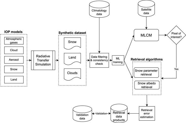
Figure 1. Flow chart of the RTM-SciML framework for snow remote sensing using satellite data.

2.1 Machine learning classification mask (MLCM)

Cloud screening is an essential first step in the satellite retrieval chain. Therefore, a Machine Learning Classification Mask (MLCM) was first applied to SGLI images to identify clear-sky overlying snow-only pixels. The current version of the SPR algorithm will be applied only to cloud-screened (clear-sky), snow-only pixels. Hence, the quality of the MLCM will control the quality of the information inferred from the SPR retrieval algorithm. The MLCM algorithm employs Scientific Machine Learning (SciML) methods (Chen et al., 2018; Baker et al., 2019; Zhou et al., 2023) in conjunction with a large synthetic dataset generated by RTM simulations for a coupled atmosphere-surface system (Chen et al., 2018; Zhou et al., 2023). This large synthetic dataset includes inherent optical property (IOP) data for a variety of aerosol and cloud (liquid water and ice) types as well as bidirectional reflectance distribution function (BRDF) data for a variety of surface types. From this MLCM tool, we obtain not only cloud-free pixels, but also a pixel-by-pixel classification of the underlying surface into several categories such as snow-only, mixed snow/vegetation (Chen et al., 2018), sea-ice, and liquid water (Zhou et al., 2023). As shown by Stillinger et al. (2019) traditional threshold-based cloud mask methods have problems over complex snow-covered terrain due to the similarity of snow and clouds in most reflectance channels as well as the surface sub-pixel mixing conditions of snow and vegetation/soil/rock. We have shown that this approach can be significantly improved through the threshold-free approach provided by the MLCM algorithm (Chen et al., 2018; Zhou et al., 2023).

The MLCM algorithm is generic in nature and could in principle be applied to any sensor with a suitable set of channels (Chen et al., 2018; Zhou et al., 2023). However, for our purpose it is important to note that our MLCM approach has been validated by collocated CALIPSO and MODIS data (Chen et al., 2014; 2018), and that it has been tailored specifically for application to the SGLI sensor. Pixels from SGLI images, classified by this MLCM algorithm as clear-sky, snow-only pixels, were used to develop and test the SPR retrieval algorithm.

2.2 Snow parameter retrieval algorithm trained by RT simulations

2.2.1 Forward model simulations and synthetic dataset generation

A comprehensive forward RTM (Stamnes et al., 2018) was used to simulate upward radiances at the top of the atmosphere (TOA). We used the sub-arctic summer atmosphere profile (Anderson et al., 1986), aerosol properties described in Supplementary Section 5.1.1.1, snow IOPs described in Supplementary Section 5.1.1.2, and a two-layer snow configuration described in Table 1. The SPR algorithm was designed with two snow layers to take into account the snow vertical structure. We fixed the thickness of the upper snow layer to be 1.5 cm and the lower layer to be 98.5 cm. Since the penetration depth for the short wavelength channels can exceed 10 cm (see Section 3.1 for details), we chose a total snow thickness of 1 m to make sure there will be no signal coming from the underlying surface. The upper layer snow thickness is within the range of the light penetration depth at the $1.64\mu$m wavelength. The snow grain size was allowed to be different in the two layers, but the impurity concentration was assumed to be the same. The snow densities were assumed to be 0.15 and 0.25 ${\mathrm{g}/\mathrm{c}\mathrm{m}}^3$ for the upper and lower snow layers, respectively. The aerosol parameters used to generate the synthetic dataset required to develop the RTM-SciML algorithm are described in Supplementary Section 5.1.1.1.

Table 1

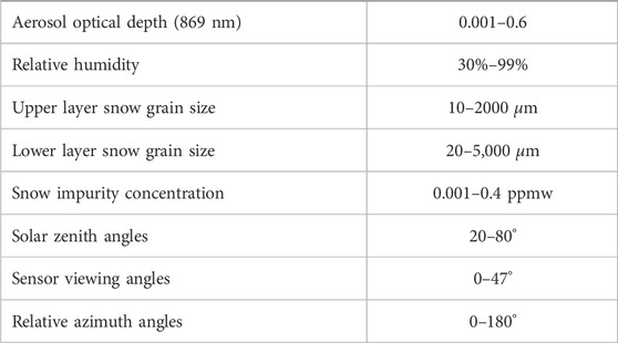
Table 1. Ranges of the parameters used to generate the MLNN training dataset. Note that the volume-to-surface-area ratio equivalent snow grain radius of a sphere is assumed for the gain size of the non-spherical snow particles. Also, for the snow impurity content a black carbon equivalent value is assumed.

The broadband albedo for each case in the synthetic dataset was also simulated in two ways. One is for blue-sky (cloud-free atmosphere) broadband albedo, and the other is for black-sky (no atmosphere) broadband albedo. Both broadband albedo values were simulated in the following 3 bands: visible (300–700 nm, VIS) albedo; near-infrared (700–3,000 nm, NIR) albedo; and shortwave (300–3,000 nm, SW) albedo. The broadband albedo can be configured to other wavelength ranges as needed.

We generated a synthetic dataset consisting of 2.7 million cases after filtering (see Section 2.2.4 for details) for the MLNN training. This dataset includes simulated TOA radiances and broadband albedo values (for blue-sky and black-sky conditions) in the VIS, NIR, and SW wavelength ranges, as well as the broadband albedo measured by instruments deployed at AWS stations, for snow and aerosol parameters as well as geometry angles appropriate for SGLI measurements. The ranges of the physical parameters and the geometry angles covered in the synthetic dataset are provided in Table 1. This table applies specifically to the conditions of the GrIS, but can easily be extended for global application.

It has been argued (Warren, 2013) that satellite remote sensing of snow impurity content (like black carbon) is unlikely to be successful, except in highly polluted industrial regions. Since the visible albedo depends on snow impurity content, we cannot ignore this effect when retrieving snow grain size (Warren and Wiscombe, 1980). Hence, we try to get information of impurity content as well (Aoki et al., 2014b), although the retrieved values are expected to have large uncertainties or may even be below the detection limit of currently available instrumentation in space for the low impurity contents encountered in pristine high-latitude regions like the Greenland Ice Sheet (GrIS) as discussed by Warren (2013).

2.2.2 Algorithm training, consistency check and output

In the SPR algorithm, we used the RTM-SciML method employing Multi-Layer Neural-Networks (MLNNs) (described below) to (i) retrieve snow and aerosol parameters; (ii) retrieve black-sky albedo and blue-sky albedo, and (iii) estimate the retrieval error. The MLNN or multilayer perceptron (MLP) is a feed-forward artificial neural network that is frequently used for pattern classification, recognition, prediction, and function approximation. It has been demonstrated that MLNNs with one or more hidden layers and a non-linear activation function can be used to approximate nonlinear functions very well (Chen et al., 1990; D’Alimonte and Zibordi, 2003; D’Alimonte et al., 2004; 2012). Therefore, they are suitable for solving our inverse problem.

The transfer (activation) function of the neurons for the MLNN was taken to be the hyperbolic tangent function:

$f\left(x\right)=\frac{2}{1+\mathrm{e}\mathrm{x}\mathrm{p}\left[-2x\right]}-1=\frac{e^x-e^{-x}}{e^x+e^{-x}}=\tanh \left(x\right).(1)$

In the output layer a linear transfer function was used to link the hidden layers to the output. The exact expression of this MLNN can be written as:

$y_m=b_{4,m}+{\displaystyle \sum _{l=1}^{N_3}}{w}_{4,ml}\cdot f\left\{b_{3,l}+{\displaystyle \sum _{k=1}^{N_2}}{w}_{3,lk}\cdot f\left[b_{2,k}+{\displaystyle \sum _{j=1}^{N_1}}{w}_{2,kj}\cdot f\left(b_{1,j}+{\displaystyle \sum _{i=1}^{N_0}}{w}_{1,ji}\cdot x_i\right)\right]\right\}(2)$

where $x_i$, $i=1,\dots ,N_0$ is an element in the input layer. It is important to note that if the goal is to make a retrieval of state parameters directly from TOA reflectance measurements, then the input parameters $x_i$ in Equation 2 are the ground elevation, the measured TOA reflectances at the seven SGLI channels plus the solar/viewing geometry, and the output parameters $y_m$ are the desired retrieval (state) parameters. We shall refer to this MLNN as R2P (Radiance $\to$ Parameter) for short. On the other hand, if the goal is to use the MLNN [Equation 2] as a fast interpolator to obtain the TOA radiances and associated Jacobians, then the input parameters $x_i$ should be the state parameters and the solar/viewing geometry, and the output parameters $y_m$ should be the TOA radiances (Stamnes and Stamnes, 2016). We shall refer to this MLNN as P2R (Parameter $\to$ Radiance) for short.

We use a 3-hidden-layer structure with $50\times 20\times$ 15 neurons for all MLNNs. In Equation 2 $w_{1,ji}$, $w_{2,kj}$, $w_{3,lk}$, and $w_{4,ml}$ are the weights of the three hidden layers and the output layer, and $b_{1,j}$, $b_{2,k}$, $b_{3,l}$, and $b_{4,m}$ are the biases of the three hidden layers and the output layer. The weights and biases are to be determined by the training. The parameter $f$ (see Equation 1) is the hyperbolic tangent function, and $y_m$ is the $m^{th}$ element in the output layer, which in the R2P case is one of the four retrieved snow and aerosol parameters (top and bottom snow grain sizes, snow impurity concentration, and aerosol optical depth); hence $m=4$. Figure 2 shows the R2P training performance with the statistical analysis values $R^2$, defined as the coefficient of determination, and the root mean square error (RMSE) value.

Figure 2

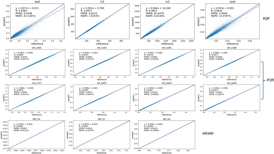
Figure 2. Training accuracy of the R2P, P2R, and albedo neural networks.

For all algorithm trainings (as listed in Figure 2), the synthetic dataset was randomly divided into two independent groups: a training group (85% of the dataset), and a validation group (15% of the dataset). The training group was used to optimize the weights and biases of the neural network and the validation group was used to validate the neural network after the training was finished. The MLNN was trained using the ‘adam’ stochastic gradient descent method (Kingma and Ba, 2017) in Scikit-Learn, which employs an adaptive learning rate (Amari et al., 2000) to reduce the training time. The training algorithm updates the weights and biases iteratively, based on the residual between the training target and the neural network output. In each iteration, the validation dataset was used to monitor the performance of the current neural network by computing the root mean square error (RMSE).

An increase in the RMSE implies that the neural network was over-trained. Therefore, the training was terminated if the RMSE increased for 10 consecutive iterations in order to avoid over-fitting. A L2 regularization scheme (Neumaier, 1998) was also applied to the training algorithm to minimize the possibility of over-fitting.

The training configurations of the R2P, P2R and albedo MLNNs are listed in Table 2. The training performance of the MLNNs is shown in Figure 2. In general, the performance is good, although the correlation coefficient $R$ for the aerosol optical depth is larger than for the other parameters, because aerosol retrieval over bright surfaces like snow is a challenging task.

Table 2

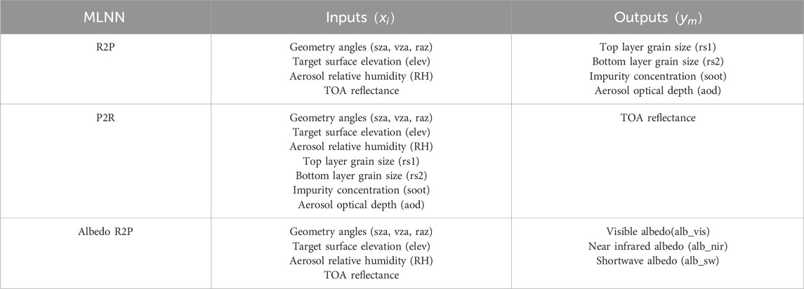
Table 2. MLNN training configurations.

2.2.3 Algorithm self-consistency and feature selection

To investigate the consistency of our trained MLNN, we apply an autoencoder neural network (aaNN) (see Section 2.2.4) between the training dataset and the satellite measurements. For this purpose, we trained a special neural network by using our simulated TOA reflectance dataset in such a way that it attempts to learn an “identity data set” (i.e., the input data are identical to the output data) with the least number of hidden layers required to create a “compressed” representation of the input.

We used satellite measured TOA reflectances as the input to this trained $R_{\text{aaNN}}$ network. If the output reflectances differ significantly from the input reflectances, it would imply that the satellite measurements are inconsistent with the radiances available in the synthetic dataset. Hence, this $R_{\text{aaNN}}$ neural network should help indicate if the algorithm is reliable, and identify other issues within the data such as instrument saturation, sensor degradation or calibration issues. A low $R_{\text{aaNN}}$ value would indicate that the simulated TOA reflectances are consistent with satellite measured data. But a high $R_{\text{aaNN}}$ value would imply that the simulated TOA reflectances are not representative of the satellite measurements, which could be an indication that the real snow is “out of the range” of (i.e., inconsistent with) our synthetic data. The reason could be that (1) the range of the synthetic dataset is not large enough to cover the different types of snow; (2) the sensor has calibration or degradation issues; (3) there are cloud screening or surface classification issues due to contamination by cloud, vegetation (or snow impurities like red algae, not considered in our forward RTM simulations), or melting snow/ice (we assumed a dry snowpack in our forward model simulations). This $R_{\text{aaNN}}$ test is performed on a channel-by-channel basis. Hence, by carefully examining the $R_{\text{aaNN}}$ values, certain channels (features) could be removed from the dataset to improve its robustness.

To generate the synthetic dataset for the $R_{\text{aaNN}}$ test, we used input layer elements consisting of the three geometry angles, the ground elevation, and the synthetic TOA reflectances in eight SGLI channels (380 nm, 412 nm, 530 nm, 674 nm, 869 nm, 1,050 nm, 1,640 nm, and 2,100 nm). The output layer elements were the TOA reflectances in these eight SGLI channels. The number of neurons for the three hidden layers were 10, 6, and 10, respectively. The $R{(i)}_{\text{aaNN}}$ is defined as follows:

$R{\left(i\right)}_{\text{aaNN}}=\left(R{\left(i\right)}_{\text{input}}-R{\left(i\right)}_{\text{output}}\right)/R{\left(i\right)}_{\text{input}}\times 100\left(\%\right)(3)$

where $i$ denotes any one of the eight SGLI channels. The $R{(i)}_{\text{input}}$ values are the original eight SGLI satellite measurements, while the $R{(i)}_{\text{output}}$ values are the eight output TOA reflectances produced by the trained autoencoder neural network.

Figure 3 shows detailed $R_{\text{aaNN}}$ values in each SGLI channel for 10-day (July 1–10, 2018) average reflectances. For a good consistency, the $R_{\text{aaNN}}$ value should be below about 5%. The largest $R_{\text{aaNN}}$ values were found to occur in the 674 nm and 530 nm channels. We found that there is a constant bias in these two channels and in the same area. The large error in the 674 nm band is due at least partly to a signal saturation issue occurring over the southern area of the GrIS. Therefore, in our snow retrieval, we excluded this channel and used only the remaining seven SGLI channels. For the 530 nm SGLI band, we conjecture that the problem may be a calibration issue, since SGLI post-launch calibration shows a 4% higher value when compared with EGRIP data (https://suzaku.eorc.jaxa.jp/GCOM_C/data/prelaunch/index_cal.html). Hence, the high positive $R_{\text{aaNN}}$ values for the 530 nm band could be due partly to the calibration bias. But, the $R_{\text{aaNN}}$ values seem to exceed 10% over the Southern GrIS (Figure 3) which might be too high to attribute solely to a calibration issue. Besides the calibration issue, the maximum radiance for the 530 nm band is designed to be 350 ${\text{Wm}}^{-2}{\text{sr}}^{-1}\mu {\text{m}}^{-1}$ which can lead to saturation over very bright targets leading to high $R_{\text{aaNN}}$ values. Due to the high reflectance of snow, these calibration/saturation issues are quite noticeable, especially over the southern area of the GrIS. For now, we continue to include the 530 nm band in our algorithm until JAXA confirms or refutes our conjecture regarding its calibration/saturation.

Figure 3

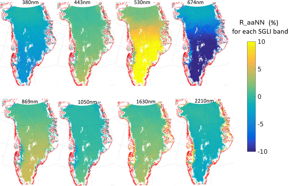
Figure 3. 10-day averaged $R_{\text{aaNN}}$ values [Equation 3] for July 1–10, 2018 for eight SGLI channels. Note: the 530 nm channel has possible calibration/saturation issues while the 674 nm channel has confirmed saturation issues.

2.2.4 Synthetic dataset filtering

To improve the performance of the SPR algorithm we proceeded as follows: Due to the sparsity of field-measured snow properties, it is challenging to generate a synthetic dataset that covers all possible situations encountered in nature. However, since the SPR algorithm is a RTM-SciML neural network based method, it is important to establish a proper training dataset, especially for the distribution and ranges of the parameters used to create this dataset. It is also important to check that the parameters have realistic relationships with each other. In order to create a realistic dataset, we adopted the following four-tiered approach:

1. We used a “random” selection of snow/aerosol parameters to establish a synthetic dataset with about 120,000 cases to train an initial P2R MLNN. We then applied this MLNN to about 120 SGLI images obtained over GrIS during two summer months of 2018 and 2019. By reviewing the retrieval results from these images, we established an appropriate range and distribution of the snow and aerosol parameters across the GrIS.

2. Based on the experience we gained by studying the snow parameters retrieved from these images, we generated a new synthetic dataset of 120,000 cases following a noncentral $F$ distribution¹ of the snow and aerosol parameters.

3. We trained an autoencoder (or auto-associative neural network, aaNN) based on MODIS MCD43A3 albedo values of July 2018 retrieved over GrIS to provide a final consistency check against real data. As described in (Fan et al. 2017; Fan et al. 2021), an autoencoder² can be used to check the consistency between two datasets and therefore it can be used to eliminate unrealistic data points in the synthetic dataset trained by MCD43 snow albedo data.

To train the autoencoder, we constructed a dataset consisting of 500,000 data points of SW, VIS, and NIR albedo values randomly selected from 2 months of MCD43 snow albedo data over GrIS and used this dataset to train the autoencoder. The low dimensionality of this albedo dataset based on only four parameters (aerosol optical depth, top layer snow grain size, bottom layer snow grain size, and snow impurity concentration) implies that it is prone to overfitting during the training of the aaNN. Here we used a 5-layer network with $4\times 15\times 4\times 15\times$ 4 neurons to construct the aaNN. Identical input and output of solar zenith angles, as well as the SW, VIS, and NIR albedo values were used in the training. The histogram of SW, VIS, and NIR albedo values of the MCD43 training dataset and the training results of the aaNN are shown in Figure 4, which indicates excellent training accuracy. Figure 4 also shows the histogram of albedo distributions of the synthetic dataset (bottom panels), which are different from those of the MCD43 data. We then applied the trained aaNN to the albedo dataset generated by using the noncentral $F$ distribution of snow parameters discussed above.

Figure 4

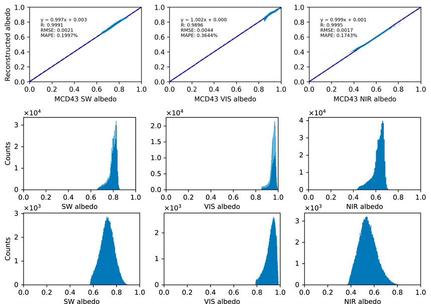
Figure 4. Top panels: Comparison of albedo reconstructed from the input data (MCD43 albedo) after passing the trained aaNN. The correlation coefficient R (the Pearson R coefficient), the root mean square of error (RMSE), mean absolute percentage error (MAPE) and correlation equation ($y=ax+b$) are shown in the legends. The solid line is the 1-1 line, and the dashed line is the fitted line by the correlation equation. Middle panels: Histograms of MCD43 albedo in SW, VIS, and NIR wavelength bands, respectively. Bottom panels: Histograms of synthetic dataset albedo in SW, VIS, and NIR wavelength bands, respectively.

The results are shown in Figure 5, which demonstrates larger dispersion and bias when passing the synthetic dataset through the aaNN trained by the MCD43 data, which indicates inconsistency between the synthetic dataset and MCD43 data. We implemented two thresholds to identify and eliminate model data that are inconsistent with the MCD43 albedo data. Hence, model data would be eliminated if 1) the percentage difference between aaNN reconstructed albedo and input albedo is greater than 2.0% for VIS, SW and NIR; 2) the VIS albedo is smaller than 0.83. The filtered model dataset shows excellent consistency with the MCD43 data with a much improved correlation and dispersion as can be seen in the bottom panels of Figure 5. The distributions of the snow parameters of this “filtered” dataset are shown in Figure 5, in which about 26.5% (31,800 cases) of the original synthetic dataset was rejected by the aaNN implying that the size of the synthetic dataset of snow parameters was reduced from 120,000 to about 90,000. We expect this new noncentral $F$ distribution dataset obtained by the procedure described above to be more realistic than a random distribution dataset, at least for conditions encountered on the GrIS during the summer season in 2018 and 2019.

4. We enlarged the filtered synthetic dataset from the previous step to be the final synthetic dataset for MLNN training. To capture snow BRDF information, for each snow case in the dataset, we generated simulated TOA reflectances at 30 viewing angle directions. Hence, the total number of cases in the synthetic dataset is about $30\times 90$,000 = 2.7 million.

Figure 5

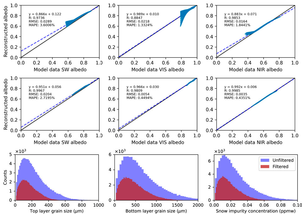
Figure 5. Top panels: A comparison of albedo reconstructed from the input data (model albedo) after passing the aaNN. Middle panels: A comparison of the reconstructed albedo and the input data (model albedo) after implementing filtering thresholds required to pass the aaNN. Bottom panels: Histogram of snow parameters for the filtered (brown) and unfiltered (blue) datasets.

One should note that the MODIS MCD43 SW albedo product pertains to the wavelength range 300–5,000 nm which is different from the wavelength range (300–3,000 nm) used in our albedo simulations. For wavelengths longer than 3,000 nm the snow albedo is extremely low (usually $<$ 0.1%) and the incoming solar irradiance is very small. Therefore, we consider the use of autoencoders trained by MCD43 albedo products justifiable in spite of the wavelength range difference.

2.2.5 Retrieval error estimation (convergence check)

In order to estimate the quality of SPR results generated by the RTM-SciML method, we first introduce a retrieval error $(R_{\text{error}})$ flag on a pixel-by-pixel basis. We use the retrieved aerosol and snow parameters to calculate the TOA reflectances [$R{(i)}_{\text{retrieved}}$ in Equation 4] at all satellite channels using a P2R MLNN as explained in Section 2.2.2. Then these computed reflectances are compared with the satellite measured ones $[R{(i)}_{\text{measured}}]$ to determine the retrieval error for channel $i$ as:

$R_{\text{error,\hspace{0.17em}i}}=\left[\left(R{\left(i\right)}_{\text{satellite}}-R{\left(i\right)}_{\text{retrieved}}\right)/R{\left(i\right)}_{\text{satellite}}\right]\times 100\left(\%\right).(4)$

The retrieval error flag is defined by averaging the $R_{\text{error,\hspace{0.17em}i}}$ over all channels:

$R_{\text{error}}=\frac{1}{{\mathrm{n}}_{\mathrm{c}\mathrm{h}}}{\displaystyle \sum _{i=1}^{{\mathrm{n}}_{\mathrm{c}\mathrm{h}}}}|R_{\text{error,\hspace{0.17em}i}}|(5)$

where ${\mathrm{n}}_{\text{ch}}$ is the number of satellite channels used in the retrieval. $R_{\text{error,i}}$ for a typical SGLI image is shown in Figure 6. It can be seen in Figure 6 that $R_{\text{error,\hspace{0.17em}i}}$ is in general below 2%–5% for most channels except for the shortwave infrared SW3 (1,630 nm) channel, which is notably wider and may have caused a larger discrepancy between simulated and measured reflectances (Chen et al., 2017). One can also find wide, slanted stripes from the composition of image from different times of the day. Although different in their absolute values, the $R_{\text{error,\hspace{0.17em}i}}$ for different channels show similar patterns as pixels with high $R_{\text{error,\hspace{0.17em}i}}$ values appear to be affected by inadequate cloud screening or melting snow. Hence we consider an averaged $R_{\text{error}}$ value of 10% to be the criterion for a “good” retrieval for SGLI.

Figure 6

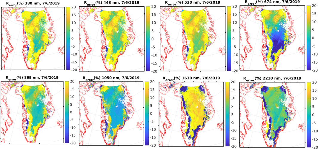
Figure 6. Retrieval error estimates [$R_{\text{error,i}}$ in Equation 4] for a SGLI image obtained over the GrIS on 6 July 2019.

3 Data, validation and application

The main focus of this paper is the development and validation of an SPR algorithm for the SGLI sensor, based on the RTM-SciML method and applied to snow-covered land areas. The MLCM and retrieval MLNNs are all trained by dry snow models, therefore the SPR algorithm is expected to be less accurate in areas affected by surface melting. Using reflectance data in seven SGLI channels (see Table 3), we developed the SPR algorithm to retrieve the snow grain size in two layers, the snow impurity concentration, the aerosol optical depth, and three broadband surface albedo values (visible (VIS), near-infrared (NIR), and shortwave (SW)) using SGLI 1 km ground resolution L1B data. To demonstrate its merits, we applied the SPR algorithm to SGLI data obtained each July from 2018 to 2021 over the GrIS. Table 3 provides a summary of the SGLI data employed by the SPR algorithm, the output standard data products from the algorithm, and the validation data.

Table 3

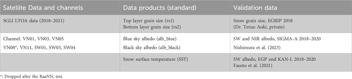
Table 3. Satellite data, output data products, and validation data employed in this study.

We used field measurements for validation of the SPR algorithm. These validation data included snow grain size data measured at the East GReenland Ice core Project (EGRIP) (Vallelonga et al., 2014) camp (75.6$°$N, 36.0$°$W, 2,708 m a.s.l.) in the central GrIS in the summer season of 2018, and surface albedo measured at the SIGMA-A site (78.1$°$N, 67.6$°$E, 1,490 m a.s.l.) (Aoki et al., 2014a) in the northwest GrIS from 2012 to 2020. The SIGMA-A site observations were conducted by members of this study (Nishimura et al., 2023). Surface albedo has been measured since July 2012 by a net radiometer (CNR-4, Kipp and Zonen, Netherlands) installed to the AWS deployed at the SIGMA-A site on the GrIS in the northwestern part of Greenland. Although the SIGMA-A station is located at the snow accumulation area, it may still be subject to surface melt and runoff during summer. To investigate the impact of surface melting on the results produced by SPR algorithm, we included the shortwave surface albedo data from the PROMICE AWS product (Fausto et al., 2021) at the EGP (accumulation) and KAN-L (ablation) field station as a comparison.

Snow samplings were performed for two snow layers of 0–2 cm and 2–10 cm at a clean area in the EGRIP camp on 30 June, 5 July, 10 July, and 15 July 2018. The snow grain size was measured for snow samples collected from a topmost layer (0–1 cm) and a thick layer (0–5 cm) using the IceCube instrument (A2 Photonic Sensors, France, Gallet et al. (2009)). This measurement was performed mainly synchronized with the overpasses of GCOM-C/SGLI. The parameter measured by the IceCube instrument is the specific surface area (SSA) ${[\text{m}}^2$ ${\text{kg}}^{-1}$] of snow grains, from which the corresponding sphere-equivalent snow grain radius (SGR) [$\mu$m] is calculated by $\mathrm{S}\mathrm{G}\mathrm{R}=3000/(\mathrm{S}\mathrm{S}\mathrm{A}{\rho }_{\text{ice}})$, where ${\rho }_{\text{ice}}$ is the ice density (0.917 g ${\text{cm}}^{-3}$) (Gallet et al., 2009). The SGR values were used to validate snow grain size retrieved from SGLI data (see Figure 7). Snow grain shapes in the top 30 cm layer consisted of faceted crystals, depth hoar, rounded grains and ice layers during the observation period. The averaged snow densities were 0.128, 0.213, 0.298 and 0.352 g ${\text{cm}}^{-3}$ for the layers of 0–3, 3–6, 6–9 and 9–30 cm, respectively. Snow surface temperature varied in the range from $-24.3°$C to $-2.6°$C. The snow samples were stored in dust-free plastic bags on site and transported to Japan. Mass concentrations of snow impurities were measured from a quartz fiber filter and a nuclepore filter on which the snow impurities were collected, in a laboratory of Meteorological Research Institute in Tsukuba, Japan using the methods employed by (Aoki et al., 2011; Aoki et al., 2014b) and Kuchiki et al. (2015). The impurity components are elemental carbon (EC) and mineral dust (MD). For the quartz fiber filters EC mass concentrations were measured with the Lab OC-EC Aerosol Analyzer (Sunset Laboratory Inc., USA) using the thermal optical reflectance method (Chow et al., 1993). The MD mass concentrations were determined by gravimetric measurements of the nuclepore filter before and after the filtration. We assumed that the component of EC is equal to black carbon (BC) for comparison with satellite-derived snow impurity mass concentrations in the present study. As satellite-inferred snow impurity mass concentrations $(c^{\text{SI}})$ contain the effects of light absorption by BC and MD, we define the BC-equivalent snow impurity mass concentration $c^{\text{SI}}$ by (Tanikawa et al., 2015).

$c^{\text{SI}}=\left(k_a^{\text{BC}}{c}^{\text{BC}}+k_a^{\text{MD}}{c}^{\text{MD}}\right)/k_a^{\text{BC}}$

where $k_a$ and $c$ are the mass absorption coefficient (in units of ${\text{m}}^2$ ${\text{g}}^{-1}$) and the impurity mass concentration (in units of g ${\text{m}}^{-3}$), respectively. We used the hydrophilic values of $k_a^{\text{BC}}=1.196\times 10^1$ ${\text{m}}^2$ ${\text{g}}^{-1}$ and $k_a^{\text{MD}}=7.389\times 10^{-2}$ ${\text{m}}^2$ ${\text{g}}^{-1}$ for the broad visible wavelength range (Aoki et al., 2011), in which the channels to retrieve snow impurity mass concentrations are contained.

Figure 7

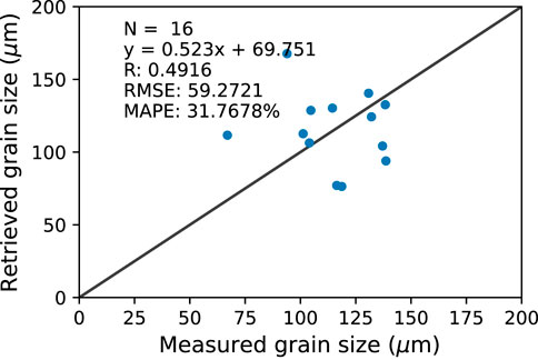
Figure 7. Comparison between satellite-derived (SGLI) snow grain sizes and field-measured ones using the IceCube instrument at the EGRIP field station for a 17-day period in July 2018.

3.1 Validation with field measurements obtained on the GrIS

We start our validation effort by comparing the satellite retrieved snow grain size to field measured SGR values in the EGRIP site. Recall that in our snow model, the upper snow layer thickness was set to 1.5 cm with snow density of $0.15\mathrm{g}{\mathrm{c}\mathrm{m}}^{-3}$, while the bottom layer was set to 98.5 cm with snow density of $0.25\mathrm{g}{\mathrm{c}\mathrm{m}}^{-3}$. These settings may not be consistent with the vertical structure of the snow during field measurements. The satellite-retrieved snow grain size depends on the light penetration depth for each channel. We calculated the penetration depth (Li et al., 2001) for a typical day (16 July 2018) from our forward RTM, using the retrieved snow and aerosol parameters as input, and found that the penetration depth is about 10 cm at the 3 shortest wavelengths, about 3.5 cm at 869 nm, about 1.5 cm at 1,240 nm, and $<1.5$ cm at 1.6 and 2.2 $\mu$m. Field IceCube measurements were obtained between 0–5 cm snow depths. Since longer wavelength ($>865$ nm) channels are more important for grain size retrieval, we consider our model setting (0–1.5 cm for the top layer, $>1.5$ cm for the bottom layer) to be comparable with the IceCube measurements.

To compare with the measurements, we averaged retrieved upper layer and lower layer snow grain sizes and compared the average value with the measured 0–5 cm value. Overall during these 18 days, the retrieved upper layer snow grain sizes were between 30 and 100 $\mu$m and the lower layer snow grain sizes were between 50 and 200 $\mu$m.

The results are shown in Figure 7 with data selected based on matching satellite measurements within 1 h time difference and satellite viewing zenith angle smaller than 30°. In total, 16 averaged snow grain size samples from 0–5 cm were selected based on these criteria. Overall, the retrieved grain size shows a positive correlation with the measurements $(R=0.49)$, but the limited sample size hampers statistical significance. Consequently, we shifted our validation efforts to in-situ snow albedo measurements, which are relatively abundant.

At the SIGMA-A site on the GrIS in the northwestern part of Greenland, albedo values were measured once a minute and 1-h averaged values were recorded. These hourly albedo values are compared with the nearest satellite-derived values ($\mathrm{\Delta }t<1$ hour) in Figure 8. The data points are color-coded by the associated averaged $R_{\text{error}}$ values from all satellite channels employed. The satellite-derived blue-sky albedo values generally agree with in-situ measurements for both SW and NIR albedo with relative errors smaller than 10%, especially for the NIR albedo which may indicate a higher accuracy in grain size retrieval. The relatively lower correlation coefficient of SW albedo may be caused by the difficulties in snow impurity retrieval, which could significantly affect the visible albedo of snow and create outliers that would significantly impact the results for a small sample size $(N=173)$. To confirm this conjecture, we re-trained the algorithm with a dataset that has impurity concentration fixed to a level that is close to that determined by the field measurements (about $2.0\times 10^3\mathrm{p}\mathrm{p}\mathrm{m}\mathrm{w}$) and repeated the retrieval. The updated results displayed in Figure 9 show that fixing the impurity concentration indeed reduced the number of outliers in SW albedo retrieval whereas the overall correlation coefficients in both SW and NIR albedo are slightly decreased. Since the NIR albedo is mainly affected by the snow grain size this finding means that the accuracy of grain size retrievals are getting worse after fixing the impurity concentration. We also noticed that the data points with large $R_{\text{error}}$ values are often located at the bottom left corner of the albedo plots, which indicates larger grain size and tendency of melting. In summary, the results show that quantifying the presence of impurity and its interaction with other parameters (especially the lower layer snow grain size) is still a challenging problem that requires further attention. The albedo enhancement under cloudy (compared to clear) sky conditions due to the change of the spectral distribution of downward irradiance over snow surfaces (Liljequist, 1956; Aoki et al., 1999) can also increase the uncertainty as the field measurements and satellite overpasses are usually not exactly simultaneous.

Figure 8

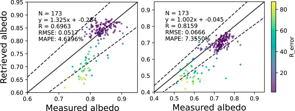
Figure 8. Comparison between SGLI albedo retrievals and ground-based albedo measurements at the SIGMA-A field station on GrIS for the months of May, June, July, and August of 2018–2020. Left panel: SW albedo. Right panel: NIR albedo. Dashed black lines represent $\pm$ 10% error range and the data points are color-coded by the associated averaged $R_{\text{error}}$ values in percent.

Figure 9

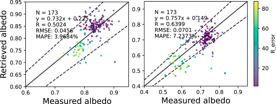
Figure 9. Same as Figure 8 but with a fixed impurity concentration in retrieval.

To further investigate the relationship between $R_{\text{error}}$ and surface melting/bare ice, we compared our retrieval results with the surface shortwave albedo data from PROMICE automatic weather station data. In the snow accumulation area of the GrIS we chose the EGP field station as this site is the only one in the PROMICE dataset that is expected to be minimally affected by surface melting as it is located at 2,660 m above the sea level and close to the center of Greenland. On the other hand, we chose the KAN-L station located in the snow ablation area to examine the performance of the algorithm when applied to mostly melting snow/bare ice surfaces. We use the same time period as that adopted for our SIGMA-A site comparison and the results are shown in Figure 10. At the EGP station, the retrieved albedo data are tightly packed between 0.8–0.9 with relatively low averaged $R_{\text{error}}$ values (with all $R_{\text{error}}$ values below 20%). The lower correlation coefficient can be explained by the “restriction of range” effect, in which the measurements (or predictions) all fall within a narrow interval so that even small amounts of scatter/noise can overshadow the true relationship and reduce the correlation. There seems to be a slight bias of satellite-retrieved albedo compared to the field measurements of about 0.03–0.05 in Figure 10. This bias could be due to the platform obstruction effect as described by (Kokhanovsky et al., 2020) which we have not attempted to correct for. We also noticed a slight difference in shortwave albedo wavelength range (0.3–2.8 $\mu \mathrm{m}$ for the SIGMA-A site and 0.3–2.5 $\mu \mathrm{m}$ for the EGP site) which we consider to be minor but leaves room for further investigation. At the KAN-L station, however, the retrieved albedo show large dispersion with significantly increased RMSE and MAPE, which indicates downgraded retrieval quality from the algorithm. The average $R_{\text{error}}$ is the largest at this site (28.36%) compared to the other sites. Detailed statistics of shortwave albedo validation are listed in Table 4.

Figure 10

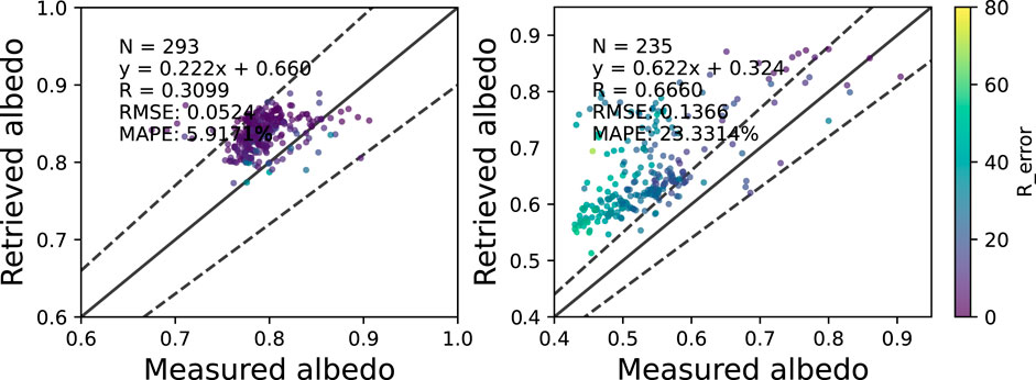
Figure 10. Comparison between SGLI shortwave albedo retrievals and ground-based shortwave albedo measurements at the PROMICE EGP (left panel) and KAN-L (right panel) field stations for the same time period as Figure 8.

Table 4

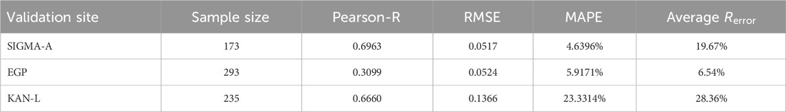
Table 4. Statistical metrics of snow shortwave albedo validation with AWS data.

3.2 Application to SGLI data over Greenland

SGLI data have been available since early 2018. In Figures 11–15, we show applications of our MLCM and SPR algorithms to SGLI data obtained over the GrIS in July of 2018, 2019, 2020, and 2021. From these data we can infer not only how the snow properties evolved during the month of July for each year, but also how the snow surface of the GrIS changed from July 2018 to July 2021.

Figure 11

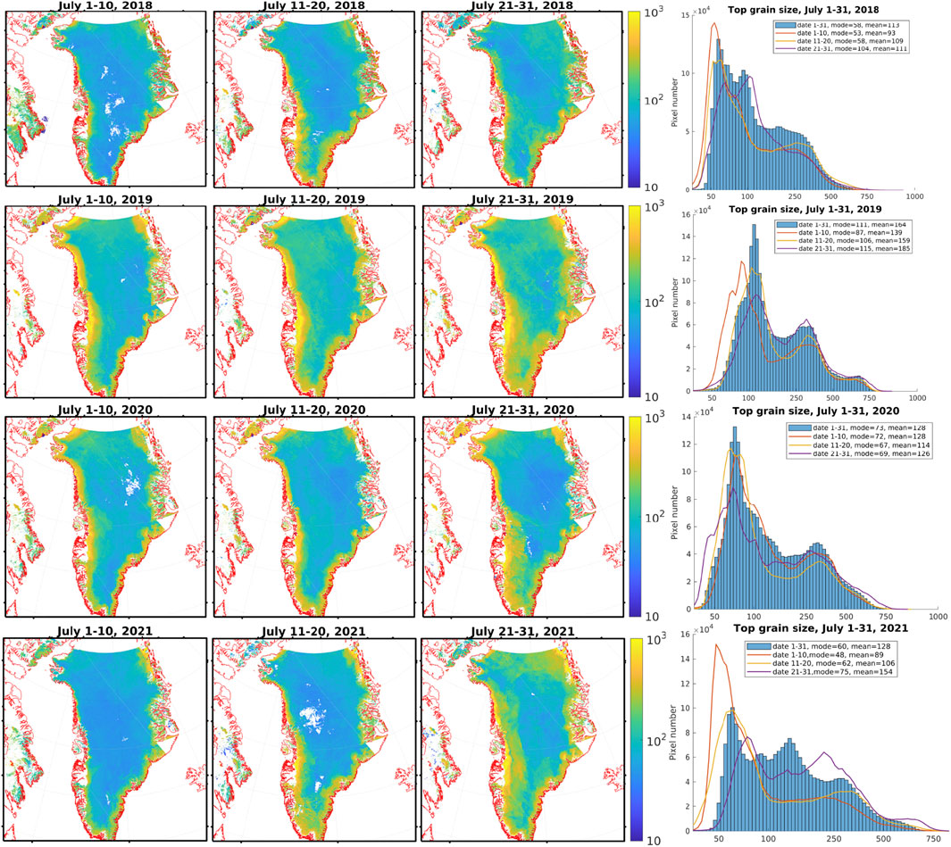
Figure 11. Comparison of 10-day averaged retrieved top layer snow grain size $(\mu \mathrm{m})$ between July of 2018–2021. The first 3 columns from left to right are for: July 1–10, July 11–20, and July 21–30 and the last panel is the histogram of the entire July. The last column displays histograms of the 10-day averages and the overall July-averaged snow retrieval parameters, with their mode and mean values indicated in the legend.

The retrieved snow grain size in the top and bottom layers of the two-layer snow configuration are shown in Figures 11, 12. The three columns from left show the 10-day average snow retrieval parameters for July 1–10, July 11–20, and July 21–30. The last column displays histograms of the 10-day averages and the overall July-averaged snow retrieval parameters, with their mode and mean values indicated in the legend. The retrieved values are smooth and stable and in basic agreement with ground truth data as demonstrated in Section 3.1. Over most of the GrIS, the upper layer snow grain size is smaller than about 100 $\mu$m, and the lower layer snow grain size is a few hundreds of $\mu$m. Although we already excluded pixels located at the edge of the GrIS identified as “non-snow’’ (by the MLCM algorithm), we still find pixels there with large grain size ($>\mathrm{1,000}\mu$m), which may be due to melting snow. At the beginning of July, the snow surface appears to be quite homogeneous across the GrIS. But later in July, a significant amount of pixels in the southern part of the GrIS has very large snow grain size ($>\mathrm{1,000}\mu$m), indicating that the snow has started to melt.

Figure 12

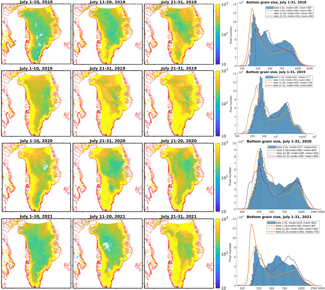
Figure 12. Same as Figure 11 but for the bottom layer grain size $(\mu \mathrm{m})$.

Among these 4 years, grain size values for July 2019 (especially for the bottom layer which is relatively stable under snow precipitation events) were found to be significantly higher with average bottom layer grain size being higher by about 54%, 25% and 27% than for the other 3 years (2018, 2020 and 2021) over the whole GrIS. This finding is consistent with Figure 15 showing that the surface temperature was also higher, implying that the GrIS was warmer in July 2019 than in July 2018, consistent with the results reported by Tedesco and Fettweis (2020) and Sasgen et al. (2020). A detailed description of the snow surface temperature product is provided elsewhere (Stamnes et al., 2007).

Consequently, both the blue sky and black sky surface albedo show lowest values for the year of 2019 compared to the other years (Figures 13, 14), with the mean blue sky and black sky albedo values for July of 2019 lowered by more than 0.02 compared to the other years. The albedo plots in Figures 13, 14, the temperature plots in Figure 15, and the $R_{\text{error}}$ plots of July 2019 in Figure 16 indicate a clear correlation between areas with lower albedo values, higher surface temperature and $R_{\text{error}}$. These results suggest that $R_{\text{error}}$ can be a good indicator of surface melting.

Figure 13

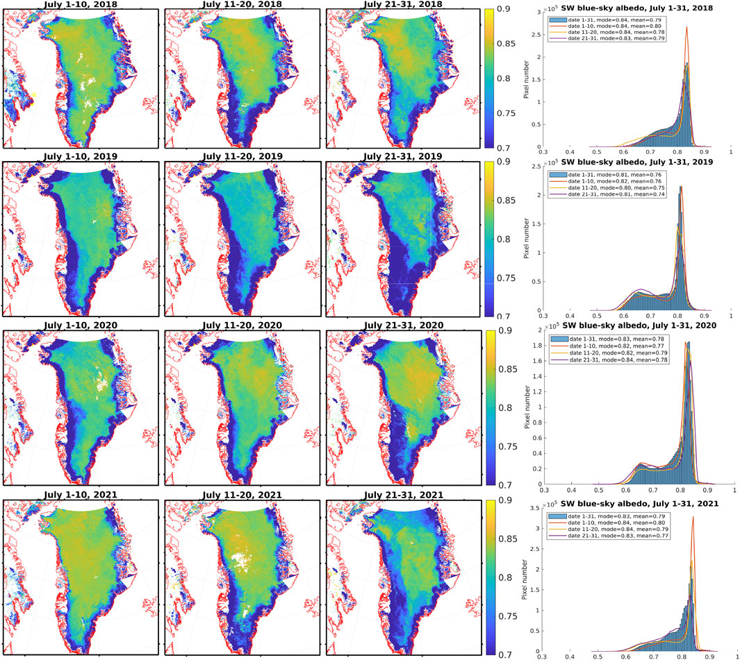
Figure 13. Same as Figure 11 but for the shortwave blue sky albedo.

Figure 14

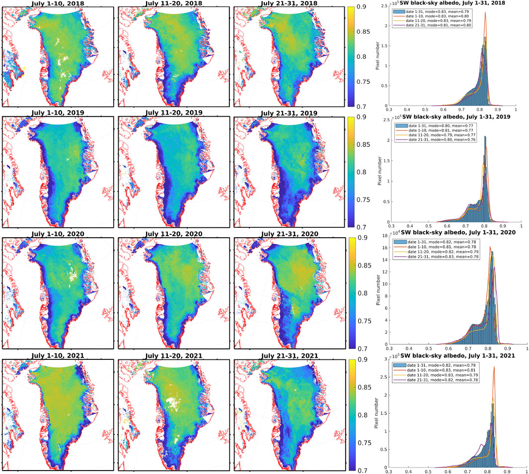
Figure 14. Same as Figure 11 but for the shortwave black sky albedo.

Figure 15

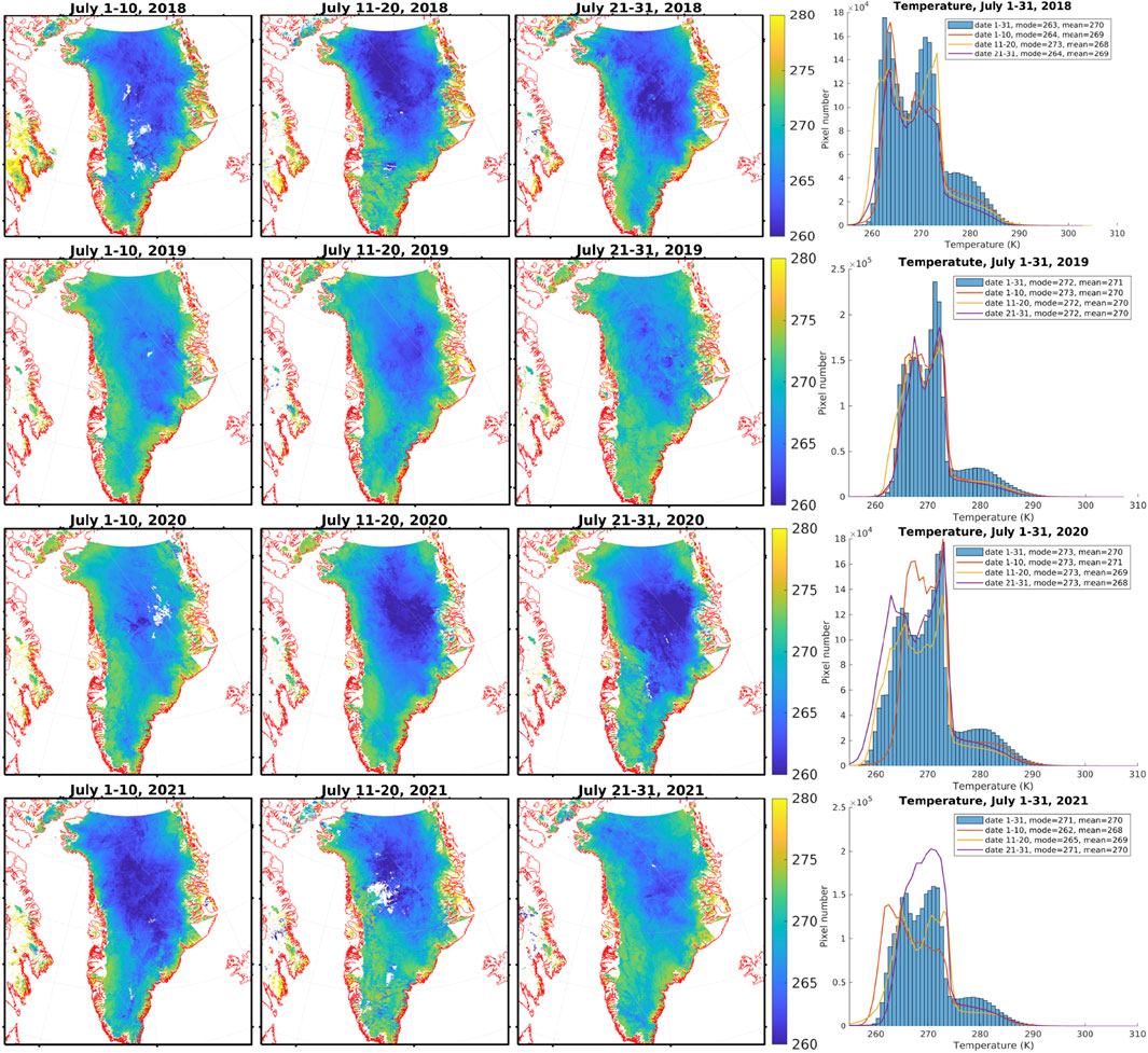
Figure 15. 10-day averaged values of snow surface temperature in Kelvin for July 2018 to July 2021.

Figure 16

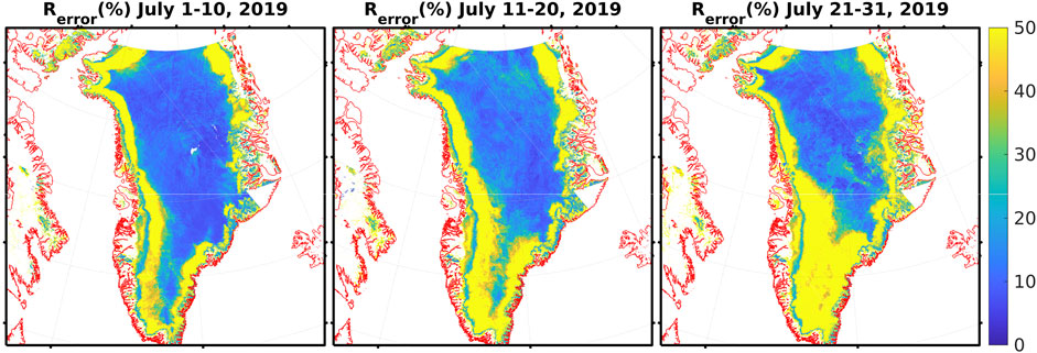
Figure 16. Comparison of 10-day averaged retrieved $R_{\text{error}}$ [Equation 5] in percentage between SGLI for July 2019. From left to right: July 1–10, July 11–20, and July 21–30.

4 Summary and conclusion

We have provided a comprehensive description of the GCOM-C SGLI Scientific Machine Learning (SciML), snow/aerosol parameter retrieval (SPR) algorithm. Overall, this SciML, neural network based SPR algorithm, provides stable and reliable retrievals of snow parameters over dry snow-covered areas. It has been applied to SGLI images and validated by field measurements. The salient features of the SPR algorithm can be summarized as follows:

1. The GCOM-C SGLI SPR algorithm provides (i) pixel-by-pixel retrievals of snow and aerosol physical parameters (two-layer snow grain size, snow impurity concentration, and aerosol optical depth); (ii) snow surface broadband albedo; (iii) consistency checks between radiative transfer model simulations and satellite measurements; and (iv) retrieval error estimates.

2. The retrieved snow grain size and albedo results are stable and reliable over dry snow-covered areas. The SPR algorithm can easily be adapted for application to different sensors with a suitable configuration of channels.

3. Impurity concentrations on the GrIS are too low to be successfully retrieved from satellite data with currently available instrumentation and methods, but could potentially be measured from space at locations with higher concentrations.

4. The SPR algorithm provides a retrieval error flag, $R_{\text{error}}$, that checks the consistency between TOA reflectances measured and computed from the retrieved snow and aerosol parameters. This flag helps establish and ensure high quality of the retrievals on a pixel-by-pixel basis and can be a good indicator of surface melting.

5. The blue-sky albedo, retrieved directly from satellite measured reflectances of cloud-free, snow-only pixels, agree well with ground-based measurements at the EGRIP and SIGMA-A sites on the GrIS.

4.1 Uncertainty estimates and future work

A future goal is to provide uncertainty estimates on a per-pixel basis, but this task is difficult for a SciML neural network designed as a regressor, which typically returns a single predicted value rather than a probability distribution. To obtain uncertainty estimates on a per-pixel basis we plan to adopt a Bayesian approach in which uncertainties in measured TOA radiances and a priori information are used to quantify uncertainties in the retrieval parameters produced by the SPR algorithm. The Bayesian uncertainty estimation algorithm is currently under development and will be implemented in future versions of the SPR algorithm. Other future work to improve the algorithm includes but is not limited to:

• Validating our algorithm using more available in-situ data (Fausto et al., 2021; How et al., 2022; Harris Stuart et al., 2023; Steen-Larsen et al., 2022; Vandecrux et al., 2022; Vandecrux et al., 2023).

• Using a “wet” snow model instead of the current dry snow model to improve the retrieval quality over areas with melting snow.

• Exploring the retrieval of snow parameters over mixed snow/vegetation areas by employing a mixed snow/vegetation canopy model.

• Exploring the potential for retrieving the presence and abundance of snow algae (like red snow).

• Employing local or regional atmospheric/aerosol profiles for specific situations (geolocation, season).

Data availability statement

The SGLI Level 2 LTOA datasets analyzed for this study and the SGLI Level 3 Cryosphere datasets generated by this study can be found in the JAXA Earth observation satellite data provision system G-Portal (https://gportal.jaxa.jp). The grain size data from EGRIP field station analyzed during the current study is privately maintained by Dr. Teruo Aoki (aoki.teruo@nipr.ac.jp). Researchers interested in accessing these data may contact Dr. Aoki via email to request permission. Quality controlled Automatic Weather Station (AWS) at SIGMA-A site can be accessed through the Arctic Data archive System (ADS) (https://doi.org/10.17592/001.2022041303). The PROMICE AWS product is available from https://doi.org/10.22008/promice/data/aws.

Author contributions

NC: Conceptualization, Data curation, Formal Analysis, Investigation, Methodology, Software, Validation, Visualization, Writing – original draft, Writing – review and editing. WL: Data curation, Formal Analysis, Methodology, Resources, Software, Validation, Visualization, Writing – original draft, Writing – review and editing. YF: Conceptualization, Methodology, Writing – review and editing. YZ: Methodology, Software, Writing – review and editing. TA: Validation, Writing – review and editing. TT: Validation, Writing – review and editing. MN: Validation, Writing – review and editing. MH: Project administration, Validation, Writing – review and editing. RS: Project administration, Validation, Writing – review and editing. SM: Validation, Writing – review and editing. KS: Conceptualization, Funding acquisition, Project administration, Writing – review and editing.

Funding

The author(s) declare that financial support was received for the research and/or publication of this article. This work was conducted as part of the Global Change Observation Mission-Climate (GCOM-C) research project of the Japan Aerospace Exploration Agency (JAXA) and the Arctic Challenge for Sustainability Project (ArCS) II (JPMXD1420318,865). Field activities to obtain the validation data were supported by the Japan Society for the Promotion of Science (JSPS) KAKENHI grant numbers of JP23221004 and JP16H01772.

Acknowledgments

We would like to thank JAXA for continual support of our work on this project. We would like to thank the EGRIP members and Kumiko-Goto Azuma who supported the validation observations at EGRIP. EGRIP is directed and organized by the Center of Ice and Climate at the Niels Bohr Institute and the US NSF, Office of Polar Programs. We would like to thank the PROMICE team members for making the PROMICE AWS products available for comparison and for valuable discussions during the peer-review process. We also would like to thank the NASA MODIS team for MODIS data and related data products, as well as the GSFC DAAC MODIS Data Support Team and the ASDC Data Management Team for making MODIS data available to the user community, which greatly helped us during the development phase of the algorithm.

Conflict of interest

The authors declare that the research was conducted in the absence of any commercial or financial relationships that could be construed as a potential conflict of interest.

Generative AI statement

The author(s) declare that no Generative AI was used in the creation of this manuscript.

Publisher’s note

All claims expressed in this article are solely those of the authors and do not necessarily represent those of their affiliated organizations, or those of the publisher, the editors and the reviewers. Any product that may be evaluated in this article, or claim that may be made by its manufacturer, is not guaranteed or endorsed by the publisher.

Supplementary material

The Supplementary Material for this article can be found online at: https://www.frontiersin.org/articles/10.3389/fenvs.2025.1541041/full#supplementary-material

Footnotes

¹This distribution is described by a quotient, where the numerator has a noncentral ${\chi }^2$ distribution with $n_1$ degrees of freedom and the denominator has a central ${\chi }^2$ distribution with $n_2$ degrees of freedom, and for which numerator and denominator are required to be statistically independent of each other. https://en.wikipedia.org/wiki/Noncentral_F-distribution.

²It is called an autoencoder neural network because it sets the target values to be equal to the inputs.

References

Amari, S., Park, H., and Fukumizu, K. (2000). Adaptive method of realizing natural gradient learning for multilayer perceptrons. Neural Comput. 12, 1399–1409. doi:10.1162/089976600300015420

PubMed Abstract | CrossRef Full Text | Google Scholar

Anderson, G. P., Clough, S. A., Kneizys, F. X., Chetwynd, J. H., and Shettle, E. P. (1986). AFGL atmospheric constituent profiles (0-120km), AFGL-TR-86-0110 (OPI) Optical Physics Division, Air Force Geophysics Laboratory. MA 01736: Hanscom AFB.

Google Scholar

Aoki, T., Aoki, T., Fukabori, M., and Uchiyama, A. (1999). Numerical simulation of the atmospheric effects on snow albedo with a multiple scattering radiative transfer model for the atmosphere-snow system. J. Meteorological Soc. Jpn. Ser. II 77, 595–614. doi:10.2151/jmsj1965.77.2_595

CrossRef Full Text | Google Scholar

Aoki, T., Kuchiki, K., Niwano, M., Kodama, Y., Hosaka, M., and Tanaka, T. (2011). Physically based snow albedo model for calculating broadband albedos and the solar heating profile in snowpack for general circulation models. J. Geophys. Res. Atmos. 116, D11114. doi:10.1029/2010jd015507

CrossRef Full Text | Google Scholar

Aoki, T., Matoba, S., Uetake, J., Takeuchi, N., and Motoyama, H. (2014a). Field activities of the snow impurity and glacial microbe effects on abrupt warming in the arctic (SIGMA) project in Greenland in 2011-2013. Bull. Glaciol. Res. 32, 3–20. doi:10.5331/bgr.32.3

CrossRef Full Text | Google Scholar

Aoki, T., Matoba, S., Yamaguchi, S., Tanikawa, T., Niwano, M., Kuchiki, K., et al. (2014b). Light-absorbing snow impurity concentrations measured on Northwest Greenland ice sheet in 2011 and 2012. Bull. Glaciol. Res. 32, 21–31. doi:10.5331/bgr.32.21

CrossRef Full Text | Google Scholar

Bair, E. H., Stillinger, T., and Dozier, J. (2021). Snow property inversion from remote sensing (SPIReS): A generalized multispectral unmixing approach with examples from MODIS and Landsat 8 oli. IEEE Trans. Geoscience Remote Sens. 59, 7270–7284. doi:10.1109/TGRS.2020.3040328

CrossRef Full Text | Google Scholar

Baker, N., Alexander, F., Bremer, T., Hagberg, A., Kevrekidis, Y., Najm, H., et al. (2019). Workshop report on basic research needs for scientific machine learning: core technologies for artificial intelligence. Tech. rep., U.S. Dep. Energy Office Sci. Tech. Inf. doi:10.2172/1478744

CrossRef Full Text | Google Scholar

Chen, N., Li, W., Gatebe, C., Tanikawa, T., Hori, M., Shimada, R., et al. (2018). New neural network cloud mask algorithm based on radiative transfer simulations. Remote Sens. Environ. 219, 62–71. doi:10.1016/j.rse.2018.09.029

CrossRef Full Text | Google Scholar

Chen, N., Li, W., Tanikawa, T., Hori, M., Aoki, T., and Stamnes, K. (2014). Cloud mask over snow/ice covered areas for the GCOM-C1/SGLI cryosphere mission: validations over Greenland. J. Geophys. Res. Atmos. 119. doi:10.1002/2014JD022017

CrossRef Full Text | Google Scholar

Chen, N., Li, W., Tanikawa, T., Hori, M., Shimada, R., Aoki, T., et al. (2017). Fast yet accurate computation of radiances in shortwave infrared satellite remote sensing channels. Opt. express 25, A649–A664. doi:10.1364/oe.25.00a649

PubMed Abstract | CrossRef Full Text | Google Scholar

Chen, S., Billings, S. A., and Grant, P. M. (1990). Non-linear system identification using neural networks. Int. J. Control 51, 1191–1214. doi:10.1080/00207179008934126

CrossRef Full Text | Google Scholar

Chow, J. C., Watson, J. G., Pritchett, L. C., Pierson, W. R., Frazier, C. A., and Purcell, R. G. (1993). The DRI thermal/optical reflectance carbon analysis system: description, evaluation and applications in US air quality studies. Atmos. Environ. Part A. General Top. 27, 1185–1201. doi:10.1016/0960-1686(93)90245-t

CrossRef Full Text | Google Scholar

D’Alimonte, D., and Zibordi, G. (2003). Phytoplankton determination in an optically complex coastal region using a multilayer perceptron neural network. IEEE Trans. Geoscience Remote Sens. 41, 2861–2868. doi:10.1109/TGRS.2003.817682

CrossRef Full Text | Google Scholar

D’Alimonte, D., Zibordi, G., and Berthon, J. F. (2004). Determination of cdom and nppm absorption coefficient spectra from coastal water remote sensing reflectance. IEEE Trans. Geoscience Remote Sens. 42, 1770–1777. doi:10.1109/TGRS.2004.831444

CrossRef Full Text | Google Scholar

D’Alimonte, D., Zibordi, G., Berthon, J.-F., Canuti, E., and Kajiyama, T. (2012). Performance and applicability of bio-optical algorithms in different European seas. Remote Sens. Environ. 124, 402–412. doi:10.1016/j.rse.2012.05.022

CrossRef Full Text | Google Scholar

Deltz, A. J., Kuenzer, C., Gessner, U., and Dech, S. (2012). Remote sensing of snow - a review of available methods. Int. J. Remote Sens. 33 (13), 4094–4134. doi:10.1080/01431161.2011.640964

CrossRef Full Text | Google Scholar

Fan, Y., Li, W., Chen, N., Ahn, J.-H., Park, Y.-J., Kratzer, S., et al. (2021). OC-SMART: a machine learning based data analysis platform for satellite ocean color sensors. Remote Sens. Environ. 253, 112236. doi:10.1016/j.rse.2020.112236

CrossRef Full Text | Google Scholar

Fan, Y., Li, W., Gatebe, C. K., Jamet, C., Zibordi, G., Schroeder, T., et al. (2017). Atmospheric correction over coastal waters using multilayer neural networks. Remote Sens. Environ. 199, 218–240. doi:10.1016/j.rse.2017.07.016

CrossRef Full Text | Google Scholar

Fausto, R. S., van As, D., Mankoff, K. D., Vandecrux, B., Citterio, M., Ahlstrøm, A. P., et al. (2021). Programme for Monitoring of the Greenland Ice Sheet (PROMICE) automatic weather station data. Earth Syst. Sci. Data 13, 3819–3845. doi:10.5194/essd-13-3819-2021

CrossRef Full Text | Google Scholar

Frei, A., Tedesco, M., Lee, S., Foster, J., Hall, D., Kelly, R., et al. (2012). A review of global satellite-derived snow products. Adv. Space Res. 50, 1007–1029. doi:10.1016/j.asr.2011.12.021

CrossRef Full Text | Google Scholar

Gallet, J.-C., Domine, F., Zender, C., and Picard, G. (2009). Measurement of the specific surface area of snow using infrared reflectance in an integrating sphere at 1310 and 1550 nm. Cryosphere 3, 167–182. doi:10.5194/tc-3-167-2009

CrossRef Full Text | Google Scholar

Harris Stuart, R., Faber, A.-K., Wahl, S., Hörhold, M., Kipfstuhl, S., Vasskog, K., et al. (2023). Exploring the role of snow metamorphism on the isotopic composition of the surface snow at EastGRIP. Cryosphere 17, 1185–1204. doi:10.5194/tc-17-1185-2023

CrossRef Full Text | Google Scholar

How, P., Lund, M., Ahlstrøm, A., Andersen, S., Box, J. E., Citterio, M., et al. (2022). PROMICE and GC-Net automated weather station data in Greenland. doi:10.22008/FK2/IW73UU

CrossRef Full Text | Google Scholar

Ishimoto, H., Adachi, S., Yamaguchi, S., Tanikawa, T., Aoki, T., and Masuda, K. (2018). Snow particles extracted from X-ray computed microtomography imagery and their single-scattering properties. J. Quantitative Spectrosc. Radiat. Transf. 209, 113–128. doi:10.1016/j.jqsrt.2018.01.021

CrossRef Full Text | Google Scholar

Ishimoto, H., Masuda, K., Mano, Y., Orikasa, N., and Uchiyama, A. (2012). Irregularly shaped ice aggregates in optical modeling of convectively generated ice clouds. J. Quantitative Spectrosc. Radiat. Transf. 113, 632–643. doi:10.1016/j.jqsrt.2012.01.017

CrossRef Full Text | Google Scholar

Kingma, D. P., and Ba, J. (2017). Adam: a method for stochastic optimization. doi:10.48550/arXiv.1412.6980

CrossRef Full Text | Google Scholar

Kokhanovsky, A., Box, J. E., Vandecrux, B., Mankoff, K. D., Lamare, M., Smirnov, A., et al. (2020). The determination of snow albedo from satellite measurements using fast atmospheric correction technique. Remote Sens. 12, 234. doi:10.3390/rs12020234

CrossRef Full Text | Google Scholar

Kokhanovsky, A., Lamare, M., Danne, O., Brockmann, C., Dumont, M., Picard, G., et al. (2019). Retrieval of snow properties from the sentinel-3 ocean and land colour instrument. Remote Sens. 11 (18), 2280–2323. doi:10.3390/rs11192280

CrossRef Full Text | Google Scholar

Kuchiki, K., Aoki, T., Niwano, M., Matoba, S., Kodama, Y., and Adachi, K. (2015). Elemental carbon, organic carbon, and dust concentrations in snow measured with thermal optical and gravimetric methods: variations during the 2007–2013 winters at sapporo, Japan. J. Geophys. Res. Atmos. 120, 868–882. doi:10.1002/2014jd022144

CrossRef Full Text | Google Scholar

Li, W., Stamnes, K., Chen, B., and Xiong, X. (2001). Snow grain size retrieved from near-infrared radiances at multiple wavelengths. Geophys. Res. Lett. 28 (1), 1699–1702. doi:10.1029/2000gl011641

CrossRef Full Text | Google Scholar

Liljequist, G. H. (1956). Energy exchange of an Antarctic snow-field: short-wave radiation. Oslo Nor. Polarinst 2.

Google Scholar

Lyapustin, A., Tedesco, M., Wang, Y., Aoki, T., Hori, M., and Kokhanovsky, A. (2009). Retrieval of snow grain size over Greenland from MODIS. Remote Sens. Environ. 113, 1976–1987. doi:10.1016/j.rse.2009.05.008

CrossRef Full Text | Google Scholar

Neumaier, A. (1998). Solving ill-conditioned and singular linear systems: a tutorial on regularization. SIAM Rev. 40, 636–666. doi:10.1137/S0036144597321909

CrossRef Full Text | Google Scholar

Nishimura, M., Aoki, T., Niwano, M., Matoba, S., Tanikawa, T., Yamasaki, T., et al. (2023). Quality-controlled meteorological datasets from SIGMA automatic weather stations in northwest Greenland, 2012–2020. Earth Syst. Sci. Data 15, 5207–5226. doi:10.5194/essd-15-5207-2023

CrossRef Full Text | Google Scholar

Painter, T., Rittger, K., McKenzie, P. S., Davis, R., and Dozier, J. (2009). Retrieval of subpixel snow covered area, grain size, and albedo from MODIS. Remote Sens. Environ. 113, 868–879. doi:10.1016/j.rse.2009.01.001

CrossRef Full Text | Google Scholar

Sasgen, I., Wouters, B., Gardner, A. S., King, M. D., Tedesco, M., Landerer, F. W., et al. (2020). Return to rapid ice loss in Greenland and record loss in 2019 detected by the GRACE-FO satellites. Commun. Earth and Environ. 1, 8. doi:10.1038/s43247-020-0010-1

CrossRef Full Text | Google Scholar

Sirguey, P., Mathieu, R., and Arnaud, Y. (2009). Subpixel monitoring of the seasonal snow cover with MODIS at 250 m spatial resolution in the Southern Alps of New Zealand: Methodology and accuracy assessment. Remote Sens. Environ. 113, 160–181. doi:10.1016/j.rse.2008.09.008

CrossRef Full Text | Google Scholar

Stamnes, K., Hamre, B., Stamnes, S., Chen, N., Fan, Y., Li, W., et al. (2018). Progress in forward-inverse modeling based on radiative transfer tools for coupled atmosphere-snow/ice-ocean systems: a review and description of the AccuRT model. Appl. Sci. 8, 2682. doi:10.3390/app8122682

CrossRef Full Text | Google Scholar

Stamnes, K., and Stamnes, J. J. (2016). Radiative transfer in coupled environmental systems: an introduction to forward and inverse modeling. John Wiley and Sons.

Google Scholar

Stamnes, K., Wei, L., Eide, H., Aoki, T., Hori, M., and Storvold, R. (2007). ADEOS-II/GLI snow/ice products: Part I - Scientific basis. Remote Sens. Environ. 111, 258–273. doi:10.1016/j.rse.2007.03.023

CrossRef Full Text | Google Scholar

Steen-Larsen, H. C., Hörhold, M., Kipfstuhl, S., Faber, A.-K., Freitag, J., Hughes, A. G., et al. (2022). 10 daily surface measurements over 90m transect, SSA, Density and Accumulation, from EastGRIP summer (May-August) of 2016-2019. doi:10.1594/PANGAEA.946763

CrossRef Full Text | Google Scholar

Stillinger, T., Roberts, D., Collar, N., and Dozier, J. (2019). Cloud masking for Landsat 8 and MODIS terra over snow-covered terrain: error analysis and spectral similarity between snow and cloud. Water Resour. Res. 55, 6169–6184. doi:10.1029/2019WR024932

PubMed Abstract | CrossRef Full Text | Google Scholar

Tanikawa, T., Kuchiki, K., Aoki, T., Ishimoto, H., Hachikubo, A., Niwano, M., et al. (2020). Effects of snow grain shape and mixing state of snow impurity on retrieval of snow physical parameters from ground-based optical instrument. J. Geophys. Res. Atmos. 125, e2019JD031858. doi:10.1029/2019JD031858

CrossRef Full Text | Google Scholar

Tanikawa, T., Li, W., Kuchiki, K., Aoki, T., Hori, M., and Stamnes, K. (2015). Retrieval of snow physical parameters by neural networks and optimal estimation: case study for ground-based spectral radiometer system. Opt. express 23, A1442–A1462. doi:10.1364/oe.23.0a1442

PubMed Abstract | CrossRef Full Text | Google Scholar

Tedesco, M. (2015). Remote sensing of the cryosphere. New York, NY, USA: Wiley.

Google Scholar

Tedesco, M., and Fettweis, X. (2020). Unprecedented atmospheric conditions (1948–2019) drive the 2019 exceptional melting season over the Greenland ice sheet. Cryosphere 14, 1209–1223. doi:10.5194/tc-14-1209-2020

CrossRef Full Text | Google Scholar

Vallelonga, P., Christianson, K., Alley, R. B., Anandakrishnan, S., Christian, J. E. M., Dahl-Jensen, D., et al. (2014). Initial results from geophysical surveys and shallow coring of the Northeast Greenland Ice Stream (NEGIS). Cryosphere 8, 1275–1287. doi:10.5194/tc-8-1275-2014

CrossRef Full Text | Google Scholar

Vandecrux, B., Box, J. E., Ahlstrøm, A. P., Andersen, S. B., Bayou, N., Colgan, W. T., et al. (2023). The historical Greenland Climate Network (GC-Net) curated and augmented level-1 dataset. Earth Syst. Sci. Data 15, 5467–5489. doi:10.5194/essd-15-5467-2023

CrossRef Full Text | Google Scholar

Vandecrux, B., Box, J. E., Wehrlé, A., Kokhanovsky, A. A., Picard, G., Niwano, M., et al. (2022). The determination of the snow optical grain diameter and snowmelt area on the Greenland ice sheet using spaceborne optical observations. Remote Sens. 14, 932. doi:10.3390/rs14040932

CrossRef Full Text | Google Scholar

Warren, S. G. (2013). Can black carbon in snow be detected by remote sensing? J. Geophys. Res. Atmos. 118, 779–786. doi:10.1029/2012jd018476

CrossRef Full Text | Google Scholar

Zege, E., Katsev, I., Malinka, A., Prikhach, A., Heygster, G., and Wiebe, H. (2011). Algorithm for retrieval of the effective snow grain size and pollution amount from satellite measurements. Remote Sens. Environ. 115, 2674–2685. doi:10.1016/j.rse.2011.06.001

CrossRef Full Text | Google Scholar

Zhou, Y., Li, W., Chen, N., Fan, Y., and Stamnes, K. (2023). A sensor-agnostic albedo retrieval method for realistic sea ice surfaces: model and validation. Cryosphere 17, 1053–1087. doi:10.5194/tc-17-1053-2023

CrossRef Full Text | Google Scholar