Gas pipeline leakage detection based on multiple multimodal deep feature selections and optimized deep forest classifier

Gas pipeline leaks contribute to one-third of methane emissions annually, posing environmental damage and safety risks. However, accurate and timely detection of the leak presents several challenges, including remote and inaccessible environments, low accuracy and efficiency, and high hardware and labor costs. To address these challenges, we propose a gas pipeline leakage detection architecture based on multiple multimodal deep feature selections and the optimized Improved Deep Forest Classifier (IDFC). First, the multimodal data, thermal images and gas sensor data, are pre-processed. Then a deep feature pool is constructed using the selected Convolutional Neural Network (CNN) models, including AlexNet, ResNet-50, MobileNet, VggNet, and EfficientNet, as well as their inner layers. Aided by the heatmaps created using Gradient-weighted Class Activation Mapping (Grad-CAM), a visualization-based primary feature selection is applied to determine the best features to form an initial CNN pool. The output of the flattened features from this CNN pool is then fed into the IDFC for classification. Hyperparameters of the base learners are then selected for an explainable and enhanced diversity tree-structured deep forest classifier, using the selected multimodal features as inputs. Finally, the Accuracy-Size Comprehensive Indicator (ASCI) is introduced for the secondary feature selection and the optimized deep forest classifier construction, which balances the model accuracy and size and reduces hardware resource requirements. Using the simulated testing dataset created for this research, our architecture demonstrated superior accuracy (98.9%) and deployability with its lower model size (115 MB). This lightweight AI architecture is successfully deployed on a soft robotic system for real-time gas leak detection. Our proposed architecture is also extensible to other environmental hazard detection situations, such as liquid leaks in the pipelines.

1 Introduction

Natural gas is becoming increasingly prevalent in the world’s energy usage, with most of it being transported through pipelines (Feijoo et al., 2018). However, statistics reveal that pipeline leaks are alarmingly frequent, occurring every 40 h in the United States alone, with many smaller leaks going unnoticed (Dutzik, 2022). These failures result in billions of dollars in damage, severe environmental contamination, and sometimes even loss of life (Williams and Glasmeier, 2022). Furthermore, pipeline leaks release nearly six million tons of methane annually (Sherwin et al., 2024), a gas which is 30 times more potent than carbon dioxide and accounts for a third of the world’s global warming due to greenhouse emissions (Environmental Protection Agency, 2023). Therefore, early detection of gas infrastructure leaks is an efficient and effective way to reduce emissions (Olczak et al., 2023).

Traditional industrial gas leak detection methods, such as hydrostatic testing and camera inspection, are often unreliable, inaccurate, costly, and labor-intensive (Fahimipirehgalin et al., 2021). External conditions, such as weather also significantly affect gas leak detection accuracy, making autonomous detection even more challenging (Zimmerle et al., 2020). As a result, there is an urgent need for a reliable system capable of inspecting gas leaks in real-time with high accuracy.

Multimodal Artificial Intelligence (AI) has been applied in gas leak detection research. Different types of data inputs, such as Acoustic Emissions (AEs) and chemical composition data, etc., are used as training inputs to create more robust Machine Learning (ML) models that withstand external disturbance for a more accurate gas leak detection result (Ullah N. et al., 2024). Recently, thermal imaging has emerged as an additional source of data for building a more robust ML architecture. Intuitively, thermal images are less prone to be affected by weather conditions such as wind, providing a data source orthogonal to the sensor data. CNNs have been the de facto ML model for image analysis since their inception (LeCun et al., 1998; Alzubaidi et al., 2021). Models such as the AlexNet (Krizhevsky et al., 2017), ResNet (He et al., 2016), MobileNet (Howard et al., 2017), and EfficientNet (Tan and Le, 2019) have been optimized for either accuracy or efficiency. Each CNN extracts different deep features, and the contribution of these features to the model’s overall performance varies. Combining these features intelligently could enhance the model’s ability to identify key areas of an image that may indicate the presence of a gas leak.

On the other hand, tree-based models and ensembles of decision trees, such as Random Forests (RFs), have been developed to improve the accuracy of predictions on numerical data (Breiman, 2001). RF, an ensemble learning algorithm, constructs multiple decision trees through bootstrap aggregation and feature randomization. The workflow comprises four key phases: (1) bootstrapped data sampling, (2) random feature selection, (3) parallel tree construction, and (4) majority-vote prediction. Specifically, during node splitting in each decision tree of the feature selection phase, the algorithm dynamically selects a random subset of features to determine optimal split criteria, thereby ensuring model diversity and mitigating overfitting. RF’s variations like the Completely Random Forest (CRF), which utilizes completely random splitting in the feature selection phase, and Mondrian Forest (MF), which partitions data space into smaller regions in the data sampling phase, aim to address challenges such as overfitting and efficiency that RFs face (Geurts et al., 2006; Lakshminarayanan et al., 2014). Additionally, boosting algorithms such as AdaBoost and eXtreme Gradient Boosting (XGBoost), which sequentially minimize error, have also been used in a wide range of applications with comparable accuracy to bagging methods (Freund et al., 1999; Chen and Guestrin, 2016). More recently, Zhou et al. proposed the Deep Forest Classifier (DFC), an ensemble learning algorithm that combines the strengths of deep learning with traditional ensemble techniques by creating a multilayer network of RFs instead of neurons or perceptrons (Zhou and Feng, 2019). However, improving the diversity of the DFC base learners to enhance model performance remains an ongoing area of research (Pan et al., 2023).

Zhang et al. introduced SPIRo (Soft Pipe Inspection Robot), a soft robot designed to adhere to and navigate pipeline surfaces, as well as a multimodal data and DFC-based AI system for gas leakage detection (Zhang and Zhang, 2024a). However, this work has several limits and disadvantages in terms of the gas leak detection model that can be improved. In this conference article, only three CNNs, specifically AlexNet, ResNet-50, and MobileNet, were employed, without adequately determining the multi-scale deep features each model extracts or exploring the performance of other possible combinations with visualization-based knowledge. Additionally, the standard DFC can be improved in terms of accuracy and efficiency by incorporating a more diverse set of base learners. Moreover, the effectiveness of the gas leak detection model has so far only been evaluated based on accuracy, but efficiency and model size are also key factors in deploying an algorithm in real-time environments.

Motivated by the issues outlined above, we propose a gas pipeline leakage detection architecture based on multiple multimodal deep feature selections and an optimized Improved DFC. First, the multimodal inputs undergo preprocessing. These inputs are then passed through the deep feature primary selection module, which selects deep features from a pool of CNNs based on feature visualization and prior knowledge. Next, the primary deep features, along with gas sensor data, are fed into the hyperparameter selection module, where the optimal hyperparameters for IDFC base learners are determined through an exhaustive grid search. Finally, using a newly defined Accuracy Size Comprehensive Indicator (ASCI), a lightweight optimized classifier is constructed with the secondary selected multimodal features and the previously obtained IDFC hyperparameters. This AI model is successfully deployed on a soft robotic system for real-time gas leak detection. The key innovations of this work are as follows: (1) A two-step deep feature selection process is developed to identify the most optimal deep features, extracted from different layers across various CNN architectures; (2) A new performance metric, the ASCI, is introduced to evaluate the trade-off between accuracy and model size for deployment on real-time embedded targets; (3) An improved deep forest classifier, incorporating a more diverse set of estimators, is proposed, demonstrating superior performance compared to other ensemble learning methods.

The structure of this article is organized as follows: Section 2 reviews the related works. Sections 3, 4 detail the algorithm development and implementation, followed by an analysis of the results. Section 5 concludes the article and suggests directions for future research.

2 Related works

2.1 Leak detection methods

Common methods of gas leak detection include chemical composition data, acoustic emissions data, and optical gas imaging (Lu et al., 2020). Chemical composition data is the most traditional and reliable method, detecting changes in the gas composition of the environment surrounding a pipeline (Lu et al., 2020). Da Cruz et al., Xiao et al., and Chi et al. implemented the acoustic method for leak detection by identifying abnormalities in sound waves produced by gas pipelines (Da Cruz et al., 2020; Xiao et al., 2019; Chi et al., 2021). Ullah, N et al. proposed a time-series-based framework leveraging AE data for pipeline leak detection (Ullah N. et al., 2024). Follow-up research employs a hybrid convolutional neural network–long short-term memory (CNN-LSTM) model for pipeline leak detection that uses AE signals as well, which achieved superior performance in higher validation accuracy and lower validation loss (Ullah S. et al., 2024). These studies experimented with various machine learning and deep learning methods, demonstrating that Support Vector Machines (SVM) and RFs achieved 99% accuracy in binary classification of simulated testing data, determining the presence of leaks. Ning et al. used a similar method to develop a status indicator for gas pipeline health (Ning et al., 2021). While both the acoustic method and chemical composition data are extensively tested, they are primarily effective when sensors are located near the leak (Lu et al., 2020).

Optical gas imaging is a relatively new field in gas leak detection that involves imaging gas plumes emitted from pipe leaks, making it more effective at sensing from a distance (Lu et al., 2020). Shi et al. and Wang et al. have tested the infrared imaging method on videos and images of field gas leaks, demonstrating the capabilities of cameras at longer distances and ranges (Shi et al., 2020; Wang et al., 2022).

Multimodal data analysis and fusion have become increasingly prevalent because they offer a more reliable method compared to previous single-modal methods. Narkhede et al., Atallah, and Azizian et al. propose a setup combining chemical composition and infrared imaging, achieving accuracies above 95% (Narkhede et al., 2021; Attallah, 2023; Azizian et al., 2024). These two data modes complement each other well in detecting gas leaks, as gas sensor data is reliable at close range while thermal imaging is versatile in various situations. However, one shortcoming of these approaches is their inefficiency in both training and inference time, making them unsuitable for real-time leak detection.

Finally, Yan et al. proposed a multisource method for detecting small gas leaks in pipeline infrastructure using pressure waves, flow, and acoustic waves. However, this method, like other acoustic sensor networks, is not successful in real field pipeline environments due to the difficulty in setup and the inability to adapt to various pipeline shapes (Yan et al., 2024).

2.2 Image feature visualization and selection

Feature extraction and visualization in CNNs and other machine learning models have long been considered a ‘black box’ due to the difficulty in understanding the basis for the models’ predictions. Saliency maps were the first widely used form of eXplainable AI (XAI) applied to image data. They determine the influence of each pixel on the final prediction by calculating the gradient of the label with respect to the input image (Simonyan et al., 2013). Since then, more XAI techniques for images have been developed, including gradient-based class activation methods. One example of such methods is Gradient-weighted Class Activation Mapping, which utilizes the gradients of the classification score with respect to the final convolutional feature map to identify the parts of an input image that most impact the classification score. These techniques use a global average pooling layer followed by the softmax function to identify the most important features for a CNN model (Selvaraju et al., 2017).

However, simply visualizing these extracted features is not sufficient to evaluate model performance. It is also necessary to select the most important features, and by extension, the most effective CNNs (Simonyan et al., 2013). The feature maps generated by different models vary because each model uses a different combination of deep layers (Oh et al., 2009). One method for selecting the feature maps to be concatenated into a final model involves visualizing these features and identifying unique ones across different models (Qian et al., 2016). This approach has proven effective because, instead of relying on an arbitrary combination of random features, it selects a diverse set of features that can each identify key focus points in an image. This reduces the impact of redundant or irrelevant features on model performance (Naheed et al., 2020). As a result, fusing different feature maps can enhance accuracy by providing a broader range of identified features from the input data (Turab et al., 2022).

2.3 Tree-based ensemble classifier

Tree-based ensemble classifiers can be categorized into two main types: bagging and boosting (Sutton, 2005). Bagging methods, such as RFs, reduce variance in ensemble tree classifiers by training each tree on a different subset of the initial dataset (Breiman, 1996). These methods offer the advantage of improved stability and the ability to handle noisy data (Breiman, 2001). On the other hand, boosting methods iteratively create predictors by focusing on correcting errors from previous iterations, thereby enhancing overall model performance (Freund et al., 1999). A key advantage of boosting is that these models are less prone to overfitting compared to bagging models because new learners are introduced with an increased degree of randomness (Freund et al., 1999).

In the field of gas leak detection, Akinsete et al. compared the effectiveness of various ensemble algorithms, including RFs, and found that ensemble decision trees were the most accurate for analyzing acoustic data (Akinsete and Oshingbesan, 2019). Zhou et al. explored the use of ensemble learning with multiple base learners in CNNs for gas leak detection and localization (Zhou et al., 2019). Kopbayev et al. further developed a spatio-temporal model that fused imaging techniques with acoustic data for inspecting gas pipes, enhancing gas leak detection (Kopbayev et al., 2022). Additionally, Wang et al. improved pipeline leakage detection accuracy by integrating a sparse autoencoder with an enhanced SVM (Wang et al., 2020).

Ensemble learning methods, such as decision trees, have been experimented with alongside deep learning approaches, including DFC, which is the chosen ensemble algorithm for this work (Zhou and Feng, 2019). The key advantage of the deep forest lies in its cascade forest structure, where other tree-based ensemble methods serve as estimators in each layer (Zhou and Feng, 2019). This structure allows the deep forest to combine the strengths of deep learning and ensemble learning, creating a more accurate alternative to traditional ensemble methods and a more efficient approach compared to conventional deep learning fusion techniques. To determine the optimal number of layers in the cascade forest, k-fold validation is employed.

However, there is still room for improvement in the accuracy and robustness of the deep forest classifier (DFC). For instance, the default base learner in the DFC is the RF, which has several disadvantages compared to more diverse methods. Primarily, the RF is more prone to overfitting than other tree-based methods. Additionally, it is relatively computationally complex, leading to longer training and prediction times. A more diverse set of base learners could be utilized to further enhance accuracy. This limitation was evident in our previous work (Zhang and Zhang, 2024b), where the unmodified DFC achieved only 88% accuracy on a simulated testing dataset due to the lack of diverse learners and the impact of overfitting on a smaller dataset.

Moreover, there remains a significant research gap in deep feature extraction and visualization within the field of gas leak detection. Current research has primarily focused on developing accurate localization and detection systems for gas leaks but has not adequately addressed the extraction of deep features used in these models. There is still a lack of understanding regarding how certain deep learning models and gas leak detection systems can be improved by optimally selecting layers and models based on the features they extract. Furthermore, it remains unclear which features are most important to each model, underscoring the need for the development of effective feature extraction methods. Ideally, these deep features should be extracted based on both model accuracy and size to ensure real-time leak detection capabilities. Finally, as demonstrated by the performance of multimodal data-based algorithms, fusing these deep features is necessary to develop the most accurate deep learning-based gas leak detection models.

3 Algorithm architecture

3.1 Algorithm framework

Based on the above analysis, a new gas pipeline leakage detection algorithm framework leveraging multiple multimodal deep feature selections and the IDFC, is proposed. It consists of four modules: the data preprocessing module, the deep feature primary selection module, the hyperparameter selection module for the IDFC, and the optimized classifier module, which incorporates secondary feature selection and comprehensive indicator. The structure of the framework is shown in Figure 1.

Figure 1

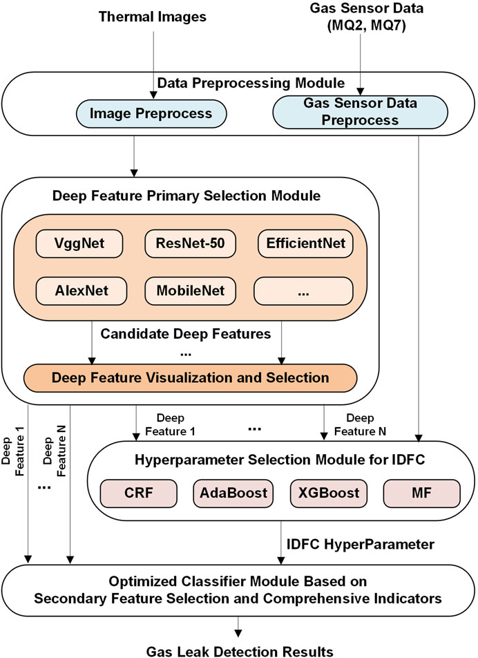
Figure 1. Algorithm framework.

The functions of the different modules illustrated in Figure 1 are described below.

(1) Data preprocessing module. The data is first pre-processed by normalization based on the same scale to remove bias among input features in different data elements. The thermal images are also unblurred to create a clearer contrast between warmer regions which indicate the presence of a gas leak and cooler regions which do not.

(2) Deep feature primary selection module. This module is responsible for developing and identifying the most optimal combination of CNNs for gas leak detection. This is achieved by generating the features of each layer of the CNNs using heatmaps and then visually determining the best deep feature layers to identify the gas leaks in the thermal images.

(3) Hyperparameter selection module for IDFC. The output from the above CNNs’ layers is applied with different tree-based IDFC to improve layer diversity. The gas sensor data is fed directly into this layer as well. The optimal hyperparameters for each base model are determined using the grid search method.

(4) Optimized classifier module based on secondary feature selection and comprehensive indicator: This module is responsible for identifying the impact of the different combinations of CNNs and their respective features, using the novel ASCI, as well as tuning hyperparameters through an exhaustive grid search, based on the leak detection accuracy of the proposed system.

3.2 Algorithm implementation

3.2.1 Data preprocessing module

The thermal images are first resized to a size of 224 × 224 × 3, reducing the computational time of the model. Then, both thermal images and gas sensor data are scaled using min-max normalization, which reduces the effects of outliers and ensures the consistency of data being passed to the machine learning model while maintaining the differences in colors for thermal images.

3.2.2 Deep feature primary selection module

3.2.2.1 Deep feature pool

CNNs are a popular machine learning model for images processing and analysis. Different CNN models were developed to extract and generate image feature maps for various use cases. Hence, leveraging the optimal models for gas leak detection can be crucial to improving the leak detection accuracy.

Each layer of each CNN generates different feature maps, as they tend to be sensitive to different areas of a RGB or grayscale image because they are built with different layers with filters. Since filters can be specialized to detect different areas of an image, each layer and filter generates different features. Thus, with more feature maps, the diversity of an ensemble model in terms of input features increases, in turn increasing model performance. Additionally, it is also important to consider the feature maps generated by the intermediate layers of each CNN. This is because most CNN architectures are built around larger datasets like ImageNet, and often, using fewer layers could provide more accurate results, especially in cases with smaller datasets, such as in the field of gas leak detection. These intermediate layers are determined through the quality of the visualized feature maps.

We propose to create a CNN feature pool and select the most effective multi-scale deep features out of the pool to build the final leak detection model. These CNNs and their features must be selected based on which combination will not only provide the most diverse and representative combination of features, but also their accuracy when it comes to leak detection through thermal image data.

In this research, we have picked five CNNs, the VggNet, ResNet-50, Mobilenet, AlexNet, and MobileNet to form the CNN pool. The pool can be extended to add more CNNs.

3.2.2.1.1 VggNet

The VggNet, or Vgg-16, is the first selected CNN used for thermal image processing. It contains 16 deep layers, uses a variety of small convolutional filters to transform the input image into a linear feature map and is one of the most commonly used CNN architectures (Alzubaidi et al., 2021). Due to the nature of each filter, the VggNet is capable of picking up on small differences in the thermal image that indicate the presence of a gas leak, allowing it to achieve high performance on image classification tasks.

3.2.2.1.2 ResNet-50

The ResNet-50 is another commonly used CNN in image classification tasks (Alzubaidi et al., 2021). ResNet-50 is a 50-layer deep CNN and can maintain the capability of generalizing data as the number of layers increases. It solves this issue through skip connections, which allows the network to skip certain layers and advance the output of a previous layer to a further layer (He et al., 2016). This allows the ResNet-50 to identify more complex features in an image and is more efficient than other similarly deep architectures.

3.2.2.1.3 EfficientNet

The EfficientNet-B3 is the third CNN added to the pool. The key difference between the EfficientNet and previous CNN architectures is the compound coefficients (Tan and Le, 2019). This allows the EfficientNet to scale layers proportionally instead of randomly as in other previous models. Finally, the EfficientNet also utilizes depth-wise convolution blocks to further enhance its efficiency over previous models. This allows the network to be capable of achieving high state of the art accuracies while simultaneously being much more efficient.

3.2.2.1.4 AlexNet

The AlexNet is another CNN added in this research, and it can extract complex features from images. It consists of a total of five convolutional max pooling layers followed by three fully connected layers, forming an 8-layer deep neural network (Krizhevsky et al., 2017). The advantages of the AlexNet lie in its ability to analyze and achieve high performance on large and diverse datasets using ReLU activation and Dropout layers. Due to its robustness, it is one of the most used CNNs in a wide range of applications, including gas leakage detection (Melo et al., 2020).

3.2.2.1.5 MobileNet

The MobileNet is the final CNN architecture that is tested in this research, with it targeting an improvement in efficiency rather than accuracy. Instead of using standard 2D convolutional layers, it uses depth-wise separable convolutions, where filters are applied to each input channel. Then, pointwise convolution is used, where the results of the previous depth-wise convolutions are combined to make a new feature (Howard et al., 2017). This allows the MobileNet to have much fewer parameters while being able to achieve similar accuracies to previous architectures.

3.2.2.2 Deep feature visualization and selection

Selecting the most optimal CNNs and their features is another crucial part of devising the most effective leak detecting system. Each CNN emphasizes different features to identify the presence of a gas leak, and selecting which features to include in the final model is essential. To visualize the features extracted by each layer of a CNN architecture, Gradient-weighted Class Activation Mapping is utilized (Selvaraju et al., 2017). Grad-CAM works by first calculating the gradient of each pixel in an image given a certain class in Equation 1:

$a_k^c=\frac{1}{Z}{\displaystyle \sum _i}{\displaystyle \sum _j}\frac{\partial y^c}{\partial {A_{ij}}^k}(1)$

where $a_k^c$ are the importance weights, ${A{x}_{ij}}^k$ are the original feature map activations derived from a convolutional layer, $Z$ is the size of the feature map, and $y^c$ is the score for the predicted class c.

Then, to retrieve a class discriminative visualization of a CNN network, a heat map $L_c$ is generated from a weighted average of the different activation maps, which is defined in Equation 2:

$L_{Grad-CAM}^c=ReLU\left({\displaystyle \sum _k}{a}_k^c{A}_k\right)(2)$

where $A^k$ are the activation maps, $a_k^c$ are the importance weights, and a ReLU is applied to eliminate features which may have a negative influence on the final prediction output.

This heatmap shows which areas of the image and which features are more important for the final prediction of a certain class. We conduct a preliminary selection of CNN features for different layers based on the visualization of these heatmaps and then select the optimal feature combination based on model accuracy when using these different features.

3.2.3 Hyperparameter selection module for IDFC

The proposed improved deep forest classifier architecture is illustrated in Figure 2.

Figure 2

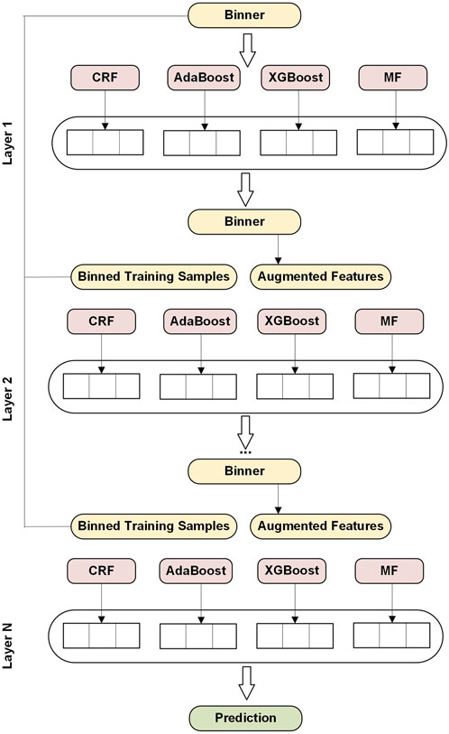
Figure 2. Improved deep forest classifier architecture.

Figure 2 illustrates that the IDFC algorithm follows a cascade forest architecture, where each layer is built upon the previous one. It functions as a deep learning network, but instead of using neurons as in a standard unit, the IDFC employs a more diverse set of base learners. The inputs to the IDFC consist of the concatenated, flattened feature maps from each CNN selected in the deep feature primary selection module, along with the gas sensor data. The data from the input layer first enters a data binner, which reduces the number of splits a decision tree must consider. The first layer of the IDFC is constructed using this binned data. Subsequently, training data for the next layers is generated by concatenating the binned predictions from the previous cascade layer with the original training samples. The performance of this new layer is then evaluated using out-of-bag samples from the original dataset. If the new layer performs better than the previous ones, another layer is added. Otherwise, the IDFC training process is terminated.

Selecting appropriate hyperparameters for different characteristic data and determining the number of layers in IDFC for various base learners is essential for enhancing model performance. The following section provides a detailed description of the principles behind these base learners and the strategy for determining the optimal number of IDFC layers.

3.2.3.1 Base learners

The base learners for the IDFC include the completely random forest, Adaboost, XGBoost, and mondrian forests. The selection criteria include the learner’s individual advantages, the diversity of the implemented base learners, as well as their tested accuracies.

3.2.3.1.1 Completely random forest

CRF is an algorithm similar to RF, which does not determine the best split for a decision tree but instead selects a random subset of split points and determines the best split among those points in the subset. The score for determining the best split is defined in Equation 3:

$Scor{e}_C\left(s,S\right)=\frac{2{I_c}^s\left(S\right)}{H_s\left(S\right)+H_c\left(S\right)}(3)$

where $S$ is a sample, $H_c$ is the log of the classification, $H_s$ is the split entropy, and ${I_c}^S$ is the mutual information of the split outcome.

The advantage of the CRF is that it introduces randomness into the RF, making it faster to train and more flexible.

3.2.3.1.2 Adaboost

The Adaboost, or adaptive boosting, algorithm is a boosting ensemble that combines multiple weak learners to create a strong ensemble algorithm. Initially, Adaboost assigns equal weight to all input features for a weak learner, such as a one-level decision tree. Then, the weak learner is trained on the data with the current weights. This error can be defined in Equation 4.

${\in }_t={\mathit{Pr}}_{i\sim D_t}\left[h_t\left(x_i\right)\ne y_i\right]={\displaystyle \sum _{i:h_t\left(x_i\right)\ne y+i}}{D}_t\left(i\right)(4)$

where $D_t\left(i\right)$ is the weight distribution on training sample $i$ at iteration $t$, $h_t$ is a weak hypothesis of a value between −1 and 1 for an instance of data, $x_i$ one sample of data from the training set, and $y_i$ is a label or result for the training data.

After training, new weights are updated based on the errors made by the weak learner, and the process is repeated iteratively. The final prediction is obtained from a majority vote of all weak learners in the model.

3.2.3.1.3 XGBoost

The XGBoost algorithm is another commonly used boosting method. Decision trees are used as the base learners, and it employs regularization techniques to improve model generalization. However, unlike the RF’s decision trees, XGBoost uses far fewer splits, resulting in shallower trees and more efficient computation. Trees are added iteratively to the model using Equation 5

$F_m\left(X\right)=F_{m-1}\left(X\right)+b_m{h}_m\left(X,r_{m-1}\right)(5)$

where $X$ is the training data, $F_m$ is the $i$ th tree in the algorithm, $b_m$ and $r_m$ are the regularization parameters, and $h_m$ is a function used to predict residuals.

The formula used to predict $b_i$ is defined in Equation 6

$\mathit{argmin}=\sum L\left(Y_i,F_{i-1}\left(X_i\right)+\alpha h_i\left(X_i,r_{i-1}\right)\right)(6)$

where $r_i$ is the residuals computed, $Y$ is the labels for the training data $X$, $L$ is a differentiable loss function, and $\alpha$ is a regularization parameter.

3.2.3.1.4 Mondrian forests

The Mondrian Forest follows a similar structure to the RF in that it is an ensemble of tree algorithms. The key difference between the MF and RF lies in how the trees are constructed. The MF generates trees using the Mondrian process, which creates splits to minimize impurity in the child nodes of a decision tree, similar to other decision trees, but without relying on labels. Mathematically, this concept can be represented Equation 7:

$C=N_{parent}Im{p}_{parent}-N_{left}Im{p}_{left}-N_{right}Im{p}_{right}(7)$

where $N$ represents the number of samples in the parent node and two child nodes, and $Imp$ is the impurity. The split is determined by drawing splits from a uniform split distribution within bounds for different feature indices rather than iterating through every possibility as with standard decision trees. This, in turn, also improves randomness and efficiency in the trees. The timing of the split in the MF is represented in Equation 8:

${\displaystyle \sum _{f=1}^D}\left(u_b\left[f\right]-l_b\left[f\right]\right)(8)$

where $D$ is the training data, $u_b$ and $l_b$ are the upper and lower bounds of all features in the particular node, and $f$ is the feature index.

The MF is constructed sequentially from multiple Mondrian trees. Compared to RFs, the MF offers the advantages of greater efficiency and the ability to operate in online environments while achieving similar accuracy. However, they are dependent on the quality of data, making them prone to overfitting on imbalanced datasets.

3.2.3.2 IDFC layer selection

The top four algorithms, based on accuracy, are selected as the four different base learners for each layer of the cascade forest, as shown in Figure 2, with every layer consisting of these four types of base learners. This approach enables the identification of the best-performing models on gas leak data and is an effective method for selecting these estimators. There are two key advantages to using these four base learners instead of relying solely on the RF. First, the efficiency of the new model is greater than that of the original DFC, which is crucial in real-time systems. Second, having more estimators in each layer improves diversity, a key factor in determining the accuracy of an ensemble model. These two factors allow the new architecture of the DFC to achieve improved performance.

3.2.3.3 Hyperparameters selection

The hyperparameters selected are based on which parameters are the most impactful to the performance of the model. To minimize the complexity of the grid search, not all parameters in these models are tested as some may have a negligible impact on the model’s final performance. In the CRF, we select the most important parameters to tune, which are the number of estimators and the number of samples needed to split a node (Geurts et al., 2006). In the Adaboost, we select all three tunable parameters, while fewer tunable parameters are chosen in the XGBoost and Mondrian Forest since these models are inherently more resistant to hyperparameter changes (Chen and Guestrin, 2016; Lakshminarayanan et al., 2014). The ranges of these parameters are estimated based on past works to reasonable bounds, where numbers too large or too small may cause overfitting and underfitting independent of what the other parameters being tuned are.

A decision tree is a non-differentiable component with significant interpretability. Ensemble-based learners, such as CRF, Adaboost, XGBoost, and Mondrian Forests, utilize multiple decision trees for prediction, which are then combined through voting decision-making. As a result, these base learners have clear and interpretable decision paths. The IDFC makes predictions through a cascade of layers, each consisting of these base learners. The output of each layer consists of a list of class probabilities from each learner, which are concatenated with the original features and passed into the next layer of the DFC. This process enables layer-by-layer learning, allowing the model to progressively refine its understanding of the data. At each layer, the full model is evaluated on a validation dataset, and the IDFC stops adding layers when validation accuracy no longer improves after a predetermined number of layers, based on the stopping criterion. In other words, the IDFC uses discrete tree splits, which allow for traceable feature importance scores. Additionally, each IDFC layer processes input features and generates new representations with explicit decision paths. Thus, the interpretability of the IDFC is derived from its unique architecture and decision-making mechanisms, offering advantages over traditional Deep Neural Networks (DNNs) in terms of transparency and feature analysis.

3.2.4 Optimized classifier module based on secondary feature selection and comprehensive indicators

The standard performance metrics for classification tasks of accuracy, precision, recall, and F1Score are utilized in this work. They are defined as in Equations 9–12:

$Accuracy=\frac{TP+TN}{TP+TN+FP+FN}(9)$

$Precision=\frac{TP}{TP+FP}(10)$

$Recall=\frac{TP}{TP+FN}(11)$

$F1=\frac{2·Precision·Recall}{Precision+Recall}(12)$

where $TP$ is the number of True Positives, $TN$ is the number of True Negatives, $FP$ is the number of False Positives, and $FN$ is the number of False Negatives.

In addition to the standard metrics, we also propose a performance metric, the ASCI, which can be defined as:

$J=W1*Accuracy+W2*\left(1-Norm\left(\mathit{ln}\left(P\right)\right)\right)(13)$

with $W1+W2=1,0<W2<W1<1$, $Norm$ representing a min-max normalization function between 0 and $\frac{1}{3}$, and $P$ being the number of parameters in the model.

ASCI defines the tradeoff between the accuracy and size for a given model. A higher J value indicates a better balance between accuracy and size, since the accuracy would be penalized more by models with more parameters and a larger size. A normalization function is required to ensure that the final P value is not too large. Different values of W1 and W2 are tested to determine the most optimal setup. Finally, to prevent significantly smaller models with lower accuracies from becoming dominant, a lower bound of the value $J$ is set based on the different values of $W1$ and $W2$, and ASCI values above this lower bound for any weights are then compared based on their accuracies, with the highest accuracy combination being the best combination. This is because each of these CNN groups has already demonstrated a relatively small size, leading to accuracy becoming the sole most important factor. The lower bound in this work is described in the results section.

3.2.5 Algorithm flow chart

The flow chart of the gas pipeline leakage detection architecture based on multiple multimodal deep feature selections and the optimized IDFC is illustrated in Figure 3.

Figure 3

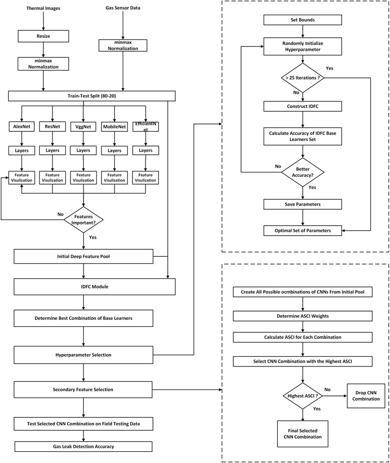
Figure 3. Flow chart of gas pipeline leakage detection architecture based on multiple multimodal deep feature selections and the optimized IDFC.

In this research, we used two major indicators for the selection of CNNs from the final deep feature pool. For the CNNs, the feature maps were analyzed to determine which CNN architectures had a stronger emphasis on the warmer region of an image itself, which would indicate the presence of a gas leak as well as the focus on the border between the warmer and cooler regions. The second major factor in deciding which CNNs to choose is the accuracy and ASCI that each can achieve on a simulated dataset. This approach allows us to select a set of accurate CNNs that each focus on a wide variety of features, increasing the probability of detecting a leak, while ensuring that the cost of this group of CNNs remains manageable.

4 Experimental results

The performance of the proposed architecture is evaluated. First, the differences between the deep feature visualizations were examined, and the model accuracy and ASCI using different weights of each CNN and different combinations of CNNs were also determined as an additional and secondary method of finding the best feature combinations. To find the optimal parameters for the IDFC and its four base learners, an exhaustive grid search was conducted to experiment with a wide range of parameters. The capabilities of the leak detection system were verified through deployment on a soft robotic system.

4.1 Soft robot integration

A compact, out of pipe soft robot is designed for transporting the apparatus necessary for facilitating gas leak detection, and further details regarding design and characterization can be found in reported work by Zhang and Zhang (2024a). The design chosen leverages the characteristics of soft robots, which have recently garnered increased attention for their deformability, adaptiveness, durability, compactness, and low cost. In contrast to rigid robots, which are suited for operation in a well-defined environment such as a factory assembly line, soft robots are able to operate in unstructured scenarios, such as gas leak detection on a pipe which may traverse different types of terrain in varying weather conditions. Thus, a soft robot is well-suited to overcome these challenges. The robot design is depicted in Figure 4a.

Figure 4

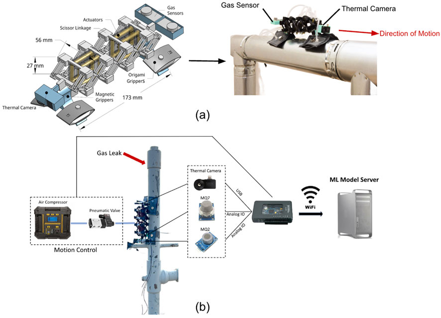
Figure 4. (a) The components and functions of the soft robot. (b) A system diagram of the soft robot and its integration in the machine learning system.

The robot’s main body and structure are composed of a compliant scissor linkage mechanism, which is labeled in Figure 4a. The scissor linkage is able to extend forward and then contract to allow the robot to locomote in an inchworm-like motion. Its material is thermoplastic polyurethane, which is flexible and allows the robot to bend itself using its actuators. It has mounting points on the front and back for straightforward switching of sensors and cameras. The robot moves through its McKibben muscle-inspired pneumatic actuators; they are placed in the locations depicted in Figure 4a, which allows their expansion to be transformed into both an extension and contraction motion. The McKibben muscles themselves are compact in size but strong when actuated and can propel the robot along both horizontal and vertical surfaces as well as maneuver the robot in tight locations. This maneuverability is also assisted by the controllability of an array of actuators; the more actuators there are, the more independent locations that can be controlled to precisely move the robot. Actuators are mounted on two positions on the robot - horizontally where they expand the body and serve as extensional actuators, and vertically where they contract the body and serve as contractional actuators for increased controllability. To attach to pipelines, the robot uses magnetic grippers, depicted in Figure 4a. The curved frame of the grippers adapts around the curvature of the pipeline to grip it, and the robot can adapt to varying diameters of piping by replacing the foot to adapt to larger or smaller diameters. The origami-inspired pouch motors are responsible for lifting and reengaging the magnets of the foot, which allows the attraction between the foot and pipe to be cut off and restarted. The pouch motors feature an origami-inspired design as seen on the gripper in Figure 4a, where the crease of the pouch motor allows the available deformation distance to be increased while the footprint of the pouch motors is kept at a minimum.

The robot has a payload capacity of 161 g, which is crucial for accommodating the sensors and apparatus necessary for gas leak detection. Specifically, for this work, three sensors are chosen for multimodal data analysis to improve the redundancy and robustness of the leak detection system and mitigate the effects of environmental disturbance. The gas composition sensors chosen are the MQ2 and MQ7 metal oxide sensors. The MQ2 sensor specifically senses for methane with a range of 100–10,000 parts per million (ppm), while the MQ7 sensor senses for carbon monoxide with a range of 20–2000 ppm. These two specific sensors were selected as they detect the two most common chemicals carried in gas pipelines.

The thermal camera utilized is capable of detecting a temperature range between −40°F to 626°F with a field of view of 46° and a resolution of 206 by 106 pixels. One significant advantage of utilizing a thermal camera is that it can penetrate smoke and dust while simultaneously detecting the heat that is emitted off them, since gas pipelines are often heated to high temperatures.

The complete system and integration of the soft robot are shown in Figure 4b. Real-time leak detection and data collection is implemented through the MyRIO microcontroller and its WIFI capabilities. Thermal images and gas sensor data are collected at 60 Hz to ensure a constant flow of up-to-date data.

4.2 Datasets

Three datasets are utilized and developed for the training and validation of the proposed algorithm framework. All three datasets either have perfect balance at 50%–50% or close to perfect balance at 45%–55% in terms of leak vs no-leak instances. Details are as follows.

The MultiModalGasData dataset was used as the initial training database and model development (Narkhede et al., 2021). It contains 3,200 instances of thermal images and their corresponding gas sensor readings for leak and no leak situations, with 1,600 of them representing the presence of a gas leak and the remaining 1,600 representing the absence of a gas leak, meaning a 50%–50% split. The data was collected using various gas chemicals commonly found in pipelines which were sprayed onto a network of sensors and a thermal camera.

The simulated testing dataset is collected by our soft robot system in a simulated pipeline leak environment designed to resemble a small section of an industrial pipeline. The environment is constructed using two sections of a metal pipe with a slight opening in between to allow the flow of air from inside the pipe to the outside environment. To simulate a no leak circumstance, data was collected purely based on atmospheric conditions. Then, a calibration gas containing 10,000 PPM of methane was passed through the pipeline with heated air to simulate the contents of the gas pipeline itself and the concentration of methane in the leak. Different amounts of gas were released through each test to simulate gas leaks of different magnitudes. This dataset contains various instances of leak and no leak situations with thermal images and their corresponding gas sensor data readings. 176 total samples were collected, with the ratio of leak to no leak data samples being 46%–54%, and the dataset was used for testing the performance of the proposed leak detection framework.

The third dataset is collected in a field environment at the Methane Emissions Technology Evaluation Center (METEC) at Colorado State University. The METEC center contains multiple pieces of retired gas infrastructure. Controlled methane emissions can be released from various points across each piece of infrastructure to simulate a gas leak. To collect data, a similar approach was utilized as in the simulated testing dataset where the soft robot and sensors were positioned on a pipeline and leaks of various magnitudes were started. Overall, data from four different leak locations on four different pieces of infrastructure were collected, amounting over 30,000 data points of gas sensor data and thermal images, with the ratio of leak to no leak data samples being 45%–55%, which were used for both training and testing in an 80:20 split.

Overall, the datasets used in this study consist of 3,200, 176, and 30,000 instances, respectively, with a class distribution of 50%–50%, 46%–54%, and 45%–55% between lean and no-lean instances. Given the requirements for modeling sample size and the balance of samples in the IDFC algorithm used in this study, we chose not to apply data augmentation to enhance model robustness. However, in future research, we plan to explore the use of this technique.

The data splitting of the various datasets are as follows. The MultiModalGasData dataset is divided into 80%:20% splits for training and testing. The simulated testing dataset is used for model testing and comparison between different architectures and layers, and the METEC data are used for evaluating the final model.

4.3 Results and discussion

4.3.1 Deep feature primary selection results

Different CNNs can extract different features from the images. In this research, five CNNs are tested to identify which features they would extract: AlexNet, ResNet-50, MobileNet-V3, VggNet, and EfficientNet-B3. We then use Grad-CAM (Selvaraju et al., 2017) to generate a visual representation of the feature maps of each CNN and its inner layers. Three sample images, representing small, medium, and large gas leaks situations respectively, are selected from the simulated testing dataset. Grad-CAM heatmaps are generated for each CNN model and its inner convolutional layers. Figure 5a shows the heatmaps for the selected layers as well as the whole CNN model tested for the sample images.

Figure 5

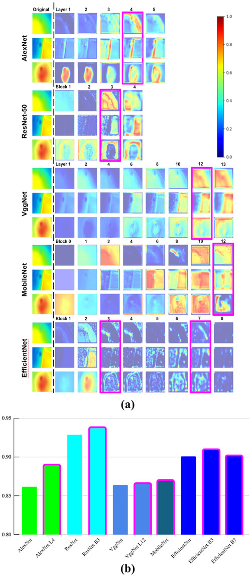
Figure 5. (a) Grad-CAM Heatmaps for Each Selected Convolutional Layer of Each CNN Model Tested for Simulated Testing Data (b) Module Accuracy of Individual CNN and it Selected Inner Layers.

As illustrated in Figure 5a, the Grad-CAM heatmaps for the selected convolutional layers of each CNN model are extracted and visualized. The color-coded bar in Figure 5a shows the relevance of the heatmap areas with 1.0 (in red) being the most relevant. Since CNNs are mostly developed to analyze regular images such as the ones from the ImageNet dataset, it is important to test and compare multiple layers from each CNN architecture because smaller subsections of a CNN’s full architecture can be more successful in gas leak detection tasks, which uses the thermal images. From the Grad-CAM heatmaps, a diverse set of features is generated for selection into the final deep feature pool. These features can be split into two main categories: (1) emphasis on the warmer part of a thermal image and (2) emphasis on the border between the warmer and cooler sections. The more accurate and representative deep features visualized from different layers of each CNN in comparison to the original image are selected for the secondary feature selection process. To determine which features would fit the best, the visualized feature maps are compared with the original image, and a manual visual comparison is conducted to identify how well the visualized feature maps correlate with the original image. Additionally, greater emphasis on a section that is indicative of a gas leak also means a more accurate feature representation because that layer then places larger emphasis on possible leak areas, leading to a higher probability of detection. For example, layer 12 of VggNet is preferred over layer 10 because it highlights areas indicative of a leak more effectively, as evidenced by the redder gradient of the heatmap.

A similar process is conducted for all architectures to determine the top two or three layers in each architecture. To maintain a diverse set of features, both models which emphasize the warmer area of the image and the border between the warmer and cooler areas are selected.

We further compare the accuracies of different layers across various CNN models and the most accurate layer from each CNN should be used in the secondary feature selection process. Figure 5b depicts the accuracy for the CNNs and selected convolutional layers tested using the simulated testing dataset. It reinforces our claim that the inner convolutional layers for a given CNN can perform better in terms of accuracy than that of the complete architecture when analyzing the thermal images. Additionally, a second sub-block from the EfficientNet is also chosen since it is one of the most accurate networks and because the visualized feature maps from two different blocks of the EfficientNet differ slightly more than other layers in other architectures.

As part of this selection process, the selected deep features include the first four layers of the AlexNet (AlexNet L4), the first three blocks of the ResNet-50 (ResNet B3), the first 12 layers of the VggNet (VggNet L12), the entire MobileNet architecture, and the first three and seven blocks of the EfficientNet (EfficientNet B3 and B7). These selections are highlighted using the pink color bonding boxes in Figures 5a,b. These six layers form the final deep feature pool, where different deep features are selected for final testing to determine the most optimal CNN block.

In summary, the ResNet and EfficientNet were the most accurate individual CNN architectures. However, it is important to note that a deeper CNN architecture, rather than sub-layers, did not always result in higher performance, partly due to the different nature of the gas thermal image dataset compared to the standard ImageNet dataset. This further demonstrates that sub-layers of CNN architectures need to be examined to determine which model fits best with thermal image data, as datasets available for gas leak detection are considerably smaller and less diverse. Additionally, the individual accuracy of each CNN is quite low, indicating the need for multimodal data analysis using both thermal images and gas sensor data.

In order to show how well the deep features are separated from each other, the t-SNE visualization is employed to the extracted features of the selected EfficientNet ResNet and VggNet algorithms. The features extracted by each layer are abbreviated by the first letter of the model’s name and the layer number (e.g., the features from the first layer of the EfficientNet would be E1). Figure 6 plots similarity of extracted features based on t-SNE visualization.

Figure 6

Figure 6. t-SNE Visualization of Similarity of Extracted Feature.

Figure 6 shows that the features extracted by each layer of different models differ significantly, with only a few obvious clusters of similar features. Thus, extracting as much information as possible from the multi-scale deep feature pool is important to maintaining diversity and accuracy in our final gas detection model. The layers that we chose are abbreviated as E7 (EfficientNet B7), R3 (ResNet B3), and V12 (VggNet L12), which represent relatively diverse areas. That is to say, they represent deep features with differences.

4.3.2 Hyperparameter selection and IDFC results

An exhaustive grid search is performed on the IDFC using the multimodal data including the selected deep feature pool and the gas sensor data. The grid search was run for a total of 25 iterations using all six top deep features determined above in the final deep feature pool. The grid search has allowed us to identify the most optimal setup for each of the base layers to fully assess the potential of the proposed leak detection architecture. The best values from this grid search were then used in the final CNN selection process and for evaluating the IDFC on field data.

Table 1 lists the tunable parameters from each learner, namely, CRF, Adaboost, XGboost and MF, the range of the grid search and its best value obtained from the search.

Table 1

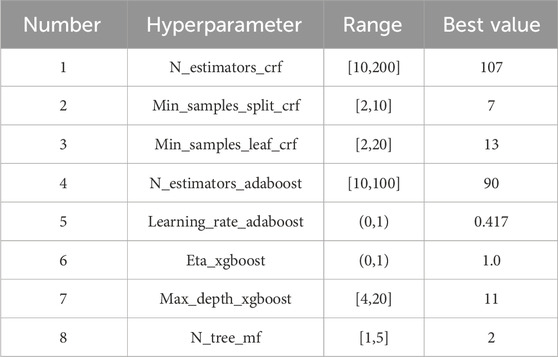
Table 1. Base learners’ hyperparameters and their ranges and the selected best values with the grid search.

The selection process of the grid search occurs in four steps: defining the parameter bound, generating parameter combinations, performing cross-validation, and selecting the best parameters. Details are as follows.

Step (1): Defining the parameter bound: These ranges and the parameters selected have been determined based on a review of past literature. For the CRF, the parameter range for the number of estimators is [10,200], the parameter range for min_samples_split is [2,10], and the parameter range for min_samples_leaf is [2,20]. For the Adaboost, the range of the number of estimators is [10,100] and the learning_rate is in range (0,1). For the XGBoost, the ETA is in range (0,1) and the max depth is in the range [4,20]. Finally, the number of trees in the Mondrian Forest is in the range [1,5].

Step (2): Generating parameter combinations: The grid search algorithm randomly selects a value in each of the ranges for each parameter. Because 25 iterations of this grid search are completed, 25 different combinations are created.

Step (3): Cross-validation for each combination: Each combination of hyperparameters for the IDFC is evaluated on the simulated testing dataset with the six features from the initial feature pool. The IDFC module receives both the feature maps from the six CNNs from the initial feature pool and the gas sensor data.

Step (4): Select the best parameters: The parameter combination which yields the best performance is selected.

The final selected value, or best value, for the selected parameter is listed in Table 1. These parameters for the base learners of the IDFC remain consistent throughout the remainder of this study.

Figure 7 depicts the accuracy of the IDFC for each additional cascade layer fitted to the model. The peak accuracy for the model occurs at four layers. Beyond this point, the accuracy will decrease for each additional layer fitted until it stabilizes around 96%. This result demonstrates that fitting more layers does not lead to higher accuracy. Hence, the standard of four layers in the IDFC method is used for the remainder of the testing.

Figure 7

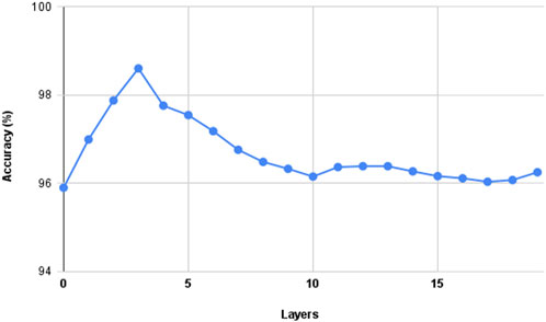
Figure 7. Accuracy for each layer in the IDFC.

Using all six deep features from the final deep feature pool and the parameters listed above in Table 1, we achieved an accuracy, precision, recall and F1Score of 0.986, 0.990, 0.991 and 0.991, respectively. This method is also more efficient than previous approaches, as it does not require powerful hardware for training and predictions. Additionally, using all six deep features results in the fusion of redundant features from different CNN architectures, with some layers extracting overlapping features. By eliminating these redundancies, it is possible to achieve even higher accuracy and further improve the algorithm’s efficiency.

4.3.3 Optimized classifier module based on secondary feature selection results

In order to determine the final selected CNN features, further comparisons of every possible combination of three CNNs is conducted, which forms 20 different CNN combinations. The combination of three CNNs is also concatenated with the MQ2 and MQ7 gas sensor data. For each of these combinations, the standard four binary classification metrics of accuracy, precision, recall, and F1Score are evaluated. On top of these performance metrics, the proposed ASCI with different weights is also evaluated to determine how efficient the method is compared to the other combinations of CNNs.

Figure 8a plots accuracies and sizes of the models under consideration. It is worth noting that there is no strong correlation between model accuracy and size. The smallest combination ResNet + EfficientNetB3+B7 in size is 48 MB, but still achieves a relatively high accuracy of 0.956, while the largest combination AlexNet L4+MobileNet + VggNet L12 in size (200 MB, 4x of the smallest one) only achieved an accuracy of 0.966, 1% better than the small size model. We can further conclude from this observation that when we prioritize a model for accuracy, such as in the gas leak detection use case, it is still possible to find a small size model that can meet the requirement and vice versa. The ASCI metric is proposed based on this finding.

Figure 8

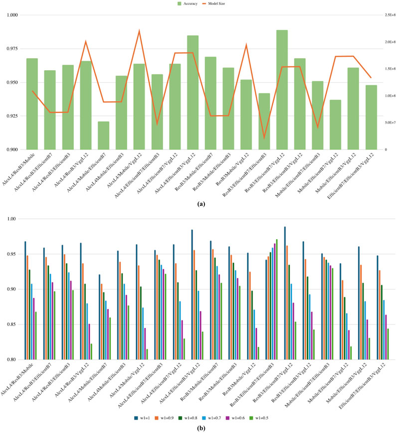
Figure 8. (a) Graph of the relationship between size and accuracy in different models (b) ASCI comparison of CNNs with different weights distribution.

We further leverage the ASCI as the secondary selection metric to further determine the best model for the gas leak detection. As mentioned earlier, ASCI is an indicator that provides guidance in trading off model accuracy and size. That is, a higher W1 in Equation 13 gives more weights on accuracy while a higher W2 puts more focus on model size. Therefore, when using the ASCI, one should determine the priority between accuracy and size based on the use case. Model size often matters when deploying the model on an embedded system where memory resource can be a constraint.

An exhaustive comparison of the ASCI values of all CNN combinations in the final deep feature pool on thermal images and gas sensor data from the simulated testing dataset is shown Figure 8b. Different weights for the ASCI metric are evaluated, but the weight of accuracy should always be greater than or equal to the weight for size, as size should not out-weight accuracy in most use cases. Once the balance of accuracy (W1) and size (W2) is determined., a higher ASCI indicates the model is preferred for such a balance. Tuning different weight values is important based on the requirements of the real-time system. We can also see that different weights have a significant effect on which models are the best in terms of the ASCI, meaning that these weights can be successfully adjusted depending on the use case.

We set the lower bound for ASCI as 0.95. For different weights, whenever the ASCI value exceeds the determined lower bound threshold, these combinations are then compared for their accuracy. The threshold of 0.95 is chosen as it filters out a significant number of models that are not efficient or accurate enough, while still retaining the top choices in terms of both accuracy and model size. Each of these unique architectures demonstrates its efficiency through relatively small penalizations in accuracy due to the model’s size.

We prioritize accuracy when picking the optimal combination for gas leak detection. Among all the combinations presented in Figure 8b, the largest memory footprint is less than 200 MB (AlexNet L4 + MobileNet + VggNet L12). Our soft robot controller, MyRIO, has 8 GB memory. Hence, it is not necessary to optimize for the model size, which allows us to pick W1 = 0.9 and W2 = 0.1 as the weights. With this decision, the combination of the first three blocks of the ResNet-50 (Resnet B3), the first seven blocks of the EfficientNet (EfficientNet B7), and the first 12 layers of the VggNet (VggNet L12) achieves the highest ASCI. Hence, this combination is determined to be the final and most optimal CNN configuration for thermal image processing.

If the model were to be deployed on hardware with less memory capacity, it is possible that more weight would need to be given to the model size. For example, W1 = 0.5 and W2 = 0.5 should be selected for hardware with memory limitations. In this case, the highest ASCI value is this weight choice for the ResNet B3, EfficientNet_B7 EfficientNet_B3 combination, which has a small model size but reasonable accuracy.

Figure 9 presents the final architecture of the proposed gas leak detection method. The complete architectures of each CNN are depicted, with arrows indicating the end of each selected convolutional layer. This architecture achieves 98.9% accuracy on simulated testing data while remaining lightweight enough to be deployable in real-time systems such as soft robots.

Figure 9

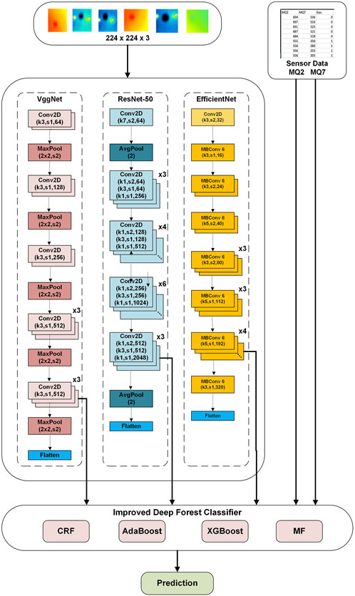
Figure 9. Final architecture of proposed gas leak detection model.

4.3.4 Leak detection model results based on METEC dataset

The proposed leak detection method has also been tested on the METEC field dataset. Figure 10 illustrates the confusion matrices of the proposed method as well as three tops performing IDFC combinations discussed above.

Figure 10

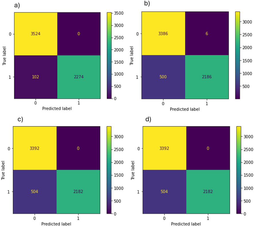
Figure 10. Confusion Matrices for (a) Proposed Method, (b) Adaboost + CRF Combination, (c) Adaboost + RF Combination, (d) Adaboost + MF Combination.

Figure 10 shows that our model outperforms the other three in all four categories in terms of TP, TN, FP, and FN. The proposed model achieves a gas leak detection accuracy of 0.954.

The overall memory consumed is 115 MB, and the latency or inference time is 0.91 s. These were evaluated on a Windows 11 CPU with an Intel I9 core processor. Thus, the relatively small memory consumption of the proposed model makes it suitable for deployment on a less powerful microcontroller device. Even though the processing speed of a microcontroller will be lower than that of a CPU, most microcontroller models, such as the MyRIO, would have sufficient processing power to run the proposed method in real-time.

The feature importance of the IDFC prediction model based on the SHapely Additive exPlanations (SHAP) technique is shown in Figure 11 (Lundberg and Lee, 2017).

Figure 11

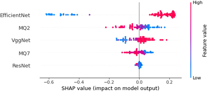
Figure 11. Feature importance of IDFC prediction model determined by SHAP analysis.

As shown in Figure 11, the thermal images provide greater weights over the gas sensor data. Among the CNN features selected for the proposed model, the EfficientNet has the greatest influence on the final gas leak detection result in terms of IDFC prediction model, followed by the MQ2 gas sensor, the VggNet, and the MQ7 gas sensor. The ResNet’s influence is almost neglectable, which could indicate that its features are not as distinctive or important to the IDFC prediction model. Overall, the thermal images and gas sensor data support each other well when improving accuracy in multimodal data analysis.

4.4 Comparison and analysis based on simulated testing datasets

4.4.1 Different methods

The comparison results of our proposed model with previous models tested with simulated testing datasets and the MultiModalGasData dataset are shown in Table 2.

Table 2

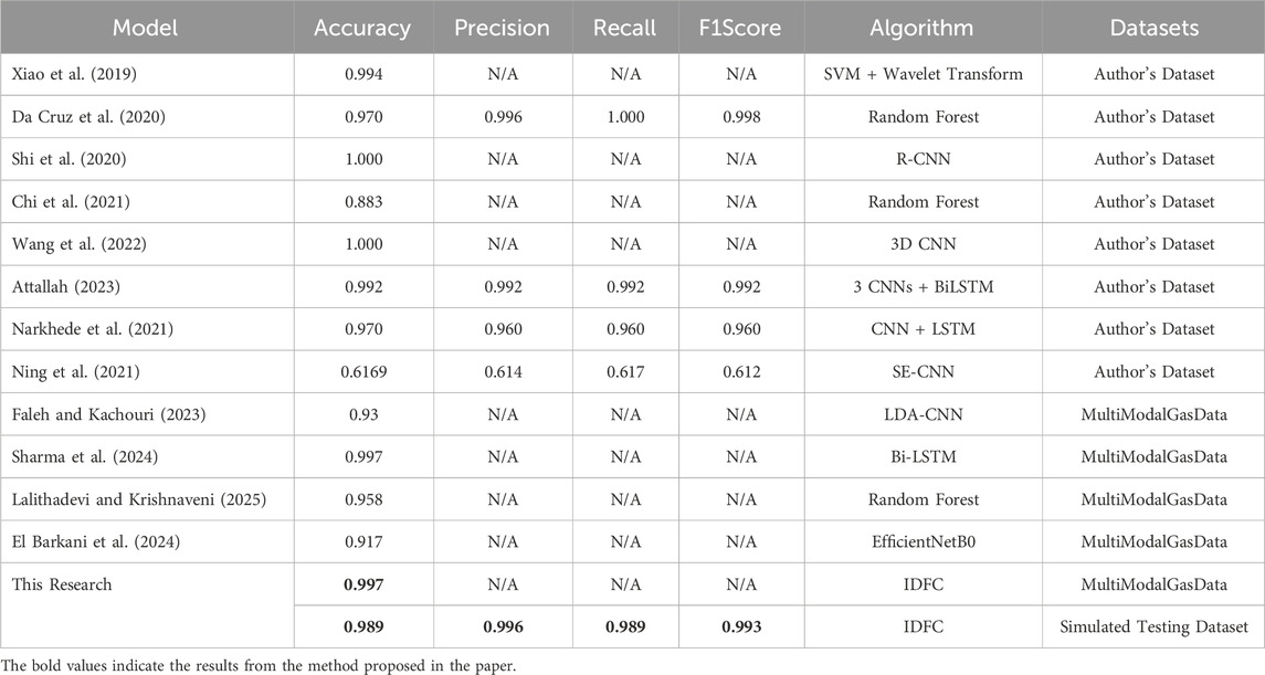
Table 2. Comparison with different methods.

In Table 2, a comparison with previous gas leak detection modules based on simulated testing datasets and the MultiModalGasData dataset proves that the proposed method is able to reach a state-of-the-art accuracy. Note that not all simulated testing datasets were identical, as each was collected by the authors of their respective algorithm. Although the accuracy achieved in this work may be slightly less than that of other previous works, the data collected at METEC in our research was collected using a soft robotic system to simulate real-time operation, causing increased variation and less consistency in our dataset and increasing the difficulty of making accurate predictions. Moreover, previous neural network-based architectures are also larger and more complex, which may also result in a slight improvement in accuracy. However, the interpretability of these deep neural network-based methods also needs to be improved. The model of the method proposed in this article is determined by a newly defined comprehensive indicator that considers both model accuracy and model size, indicating that the constructed model is more applicable. Thus, the model requires less training time with the capability to be deployed in real-time embedded systems. Most previous works require the need for extensive hardware to be effectively deployed, while the proposed method is more lightweight than previous methods because of the use of the IDFC as a result of the comparison using the ASCI indicator. Thus, this allows it to be deployed on remote or low-cost systems equipped with basic hardware and microcontrollers, advancing the field of gas leak prevention and reducing the impact of methane emissions on the environment.

Table 2 also shows the comparison results with more recent state-of-the-art methods based on MultiModalGasData dataset. Our model achieved the highest accuracy with 0.997, along with the results from Sharma et al. (2024) However, the model of the latter is constructed with Bi-LSTM, which lacks interpretability. Moreover, many methods in these literatures only use datasets for model accuracy validation and do not consider hardware implementation. This demonstrates that our model is both accurate and efficient.

4.4.2 Model performance with different DFC variations

Table 3 demonstrates the performance of different combinations of estimators in each layer of the DFC.

Table 3

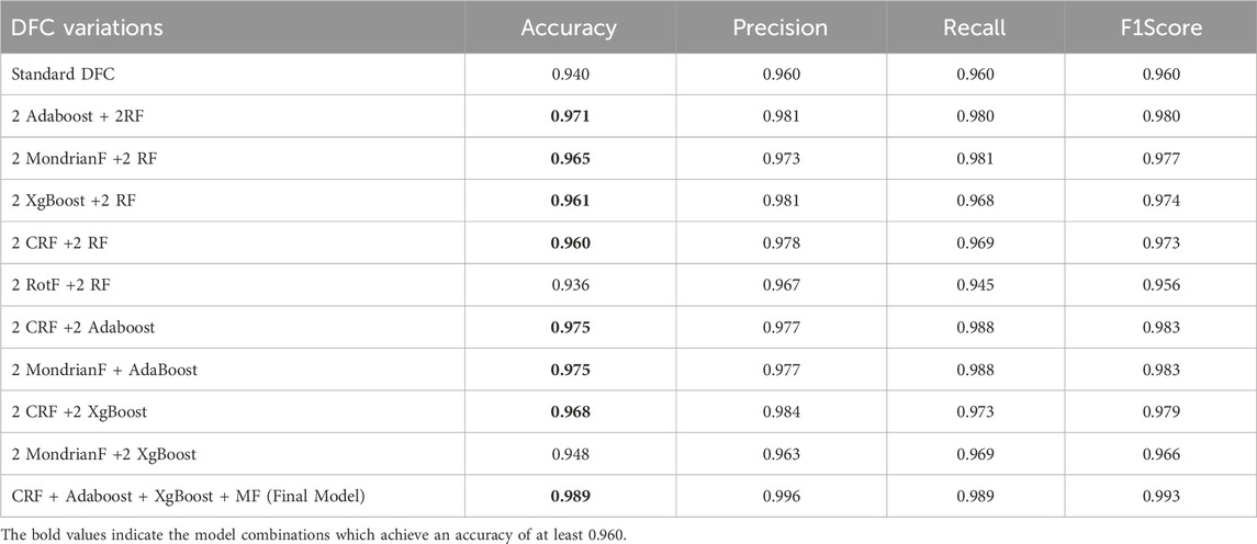
Table 3. Comparison of different DFC Variations.

In Table 3, Changing the estimators utilized in the IDFC module has several advantages, but the most optimal combination again needs to be determined, as the original DFC using only RFs and CRFs achieves the second lowest accuracy of 0.940. This is due to the high likelihood of overfitting in the random forest on relatively smaller datasets. Therefore, the proposed method must be both efficient for real-time leak detection and accurate by preventing overfitting and creating a more diverse ensemble of learners. Table 3 also shows that using two boosting estimators along with the random forest achieves a significantly higher accuracy of 0.96–0.97. A similar level of accuracy is achieved with MF and CRF. Thus, as CRF, MF, Adaboost, and XGBoost achieve the highest accuracy among themselves and the random forest, they are combined in one layer of the DFC, further demonstrating the success of the proposed IDFC.

4.4.3 Training and inference time with different DFC variations

The training and inference times of different DFC variations are shown in Table 4.

Table 4

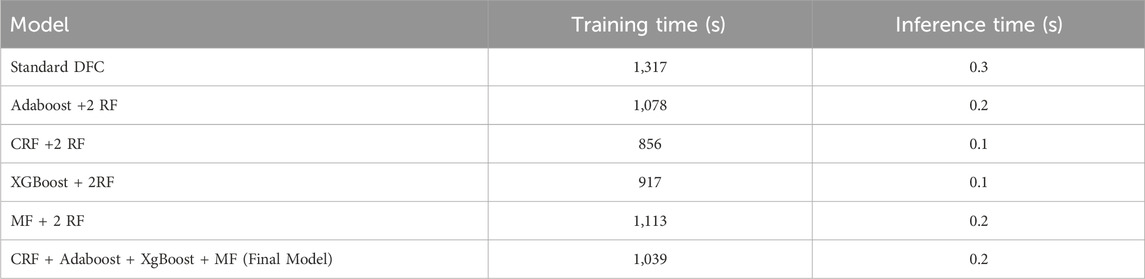
Table 4. Training times of each cascade forest with modified layers.

From Table 4, it is evident that the proposed alternative to the DFC, with a training time of 1,039 s, is more efficient than the original standard DFC but not as efficient as other DFC variations. This reduced efficiency is due to the need for more computations with four different learners. However, this slight decrease in efficiency is offset by an improvement in accuracy. The proposed method achieves a 1% higher accuracy on the simulated testing dataset, and this improvement will only be compounded in field environments.

4.5 Comprehensive analysis

As mentioned earlier, around six million tons of methane is released into the earth’s atmosphere annually due to gas pipeline leaks, accounting for ⅓ of greenhouse gases that contribute to global warming. On the other hand, gas pipelines traverse remote landscapes or complex environments that are not easily accessible, making leak detection even more challenging. Our proposed architecture, which can be deployed on a soft robot due to its lightness both in compute power and memory footprint, has the potential of enabling early detection of methane leaks and eliminating ⅓ of the greenhouse gas if actions are taken timely.

Additionally, our proposed framework of constructing the optimal model for gas leak detection is generic and extensible to other types of environmental hazard detection scenarios. By building different images and sensor datasets for a given scenario, different optimal CNN features pool can be selected. Furthermore, a different set of the base learners can be determined using the same proposed approach to form the IDFC. After that, ASCI can guide the user to determine the best model to fit the accuracy and deployment constraints.

As an example, consider we need to detect the liquid pipeline leaks. We can change the thermal imaging camera to a regular RGB image camera with a different set of sensors that can capture the leaked liquid characteristics. Once a dataset is built with these images and sensor data, the same analysis can be applied to detect liquid pipeline leaks and the final model can be deployed on the soft robot described earlier.

5 Conclusion

This article proposes a lightweight multimodal machine learning architecture based on CNNs and deep forest classifiers for gas pipeline leak detection systems using thermal image and gas sensor data. The architecture consists of an optimal CNN features pool, an improved deep forest classifier with four base learners, and a secondary CNN feature selection module for the final model. This novel framework not only considers the model accuracy but also the model deployability on the gas leak detecting platform, a soft robot, which has limited computer power and memory capacity. To our knowledge, this is the first proposed end-to-end methodology with such consideration in the area of gas leak detections. Our contributions in this research can be summarized as follows:

• The deep features of the multiple convolutional layers, as well as the full architecture of CNNs, including AlexNet, ResNet, VggNet, MobileNe,t and EfficientNet, are examined using heatmaps. Our results demonstrated that the inner layers with different scale can be more effective in detecting the thermal images for gas leak. This leads to creating a CNN feature pool that consists of multi-scale deep features of the selected CNNs.

• An improved deep forest classifier with a more diverse set of base learners, including CRF, Adaboost, XGBoost, and MondrianF, is proposed. An exhaustive search for the optimal parameters for each base learner is performed. We showed that the combination of the four base learners in the IDFC achieved higher accuracy than the standard DFC.

• We employed a secondary selection mechanism to avoid feature overlaps in the selected CNN feature, hence further trimming down the model size without loss of the model accuracy. This makes the model more suitable to be deployed on an embedded system like the soft robot.

• The novel ASCI indicator is proposed to determine the multi-scale deep feature from the CNN pool that best fit the gas leak detection use case, balancing the model accuracy and size. Depending on the deployment requirements, a different combination of models can be selected based on the ASCI indicator.

Our results demonstrate the robustness of the proposed method, with the algorithm achieving an accuracy of 98.9% on the simulated testing dataset, matching the performance capabilities of previous works with only ⅓ of the model size reported from that work. However, we are also able to maintain an ASCI score of above 0.95 on multiple models, demonstrating the smaller size of our algorithm and its ability to be deployed on real-time systems. The method is tested in a field environment and can still attain accuracies of over 95.4%.

Future directions of this research include (1) constructing a large gas leak dataset including thermal images and gas sensor data from the gas pipeline field to improve the accuracy of the trained model; (2) extend the proposed multi-scale deep feature CNN pool to include more CNN architecture; and (3) update the IDFC to include more base learners to allow the architecture to deal with more diverse dataset.

Data availability statement

The raw data supporting the conclusions of this article will be made available by the authors, without undue reservation.

Author contributions

EdZ: Conceptualization, Data curation, Formal Analysis, Investigation, Methodology, Resources, Software, Validation, Visualization, Writing – original draft, Writing – review and editing. EvZ: Conceptualization, Data curation, Investigation, Methodology, Resources, Validation, Writing – review and editing.

Funding

The author(s) declare that no financial support was received for the research and/or publication of this article.

Conflict of interest

The authors declare that the research was conducted in the absence of any commercial or financial relationships that could be construed as a potential conflict of interest.

Generative AI statement

The author(s) declare that no Generative AI was used in the creation of this manuscript.

Publisher’s note

All claims expressed in this article are solely those of the authors and do not necessarily represent those of their affiliated organizations, or those of the publisher, the editors and the reviewers. Any product that may be evaluated in this article, or claim that may be made by its manufacturer, is not guaranteed or endorsed by the publisher.

References

Akinsete, O., and Oshingbesan, A. (2019). “Leak detection in natural gas pipelines using intelligent models,” in SPE Nigeria annual international conference and exhibition.

Google Scholar

Alzubaidi, L., Zhang, J., Humaidi, A. J., Al-Dujaili, A., Duan, Y., Al-Shamma, O., et al. (2021). Review of deep learning: concepts, CNN architectures, challenges, applications, future directions. J. Big Data 8, 53. doi:10.1186/s40537-021-00444-8

PubMed Abstract | CrossRef Full Text | Google Scholar

Attallah, O. (2023). Multitask deep learning-based pipeline for gas leakage detection via e-nose and thermal imaging multimodal fusion. Chemosensors 11 (7), 364. doi:10.3390/chemosensors11070364

CrossRef Full Text | Google Scholar

Azizian, A., Yousefimehr, B., and Ghatee, M. (2024). “Enhanced multi-modal gas leakage detection with nsmote: a novel over-sampling approach,” in 2024 8th international conference on smart cities, internet of things and applications (SCIoT).

Google Scholar

Breiman, L. (1996). Bagging predictors. Mach. Learn 24, 123–140. doi:10.1007/BF00058655

CrossRef Full Text | Google Scholar

Breiman, L. (2001). Random forests. Mach. Learn. 45, 5–32. doi:10.1023/A:1010933404324

CrossRef Full Text | Google Scholar

Chen, T., and Guestrin, C. (2016). “XGBoost: a scalable tree boosting system,” in 22nd ACM SIGKDD international conference on knowledge discovery and data mining.

Google Scholar

Chi, Z., Li, Y., Wang, W., Xu, C., and Yuan, R. (2021). Detection of water pipeline leakage based on random forest. J. Phys. Conf. Ser. 1978, 012044. doi:10.1088/1742-6596/1978/1/012044

CrossRef Full Text | Google Scholar

Da Cruz, R. P., Vasconcelos da Silva, F., and Frattini Fileti, A. M. (2020). Machine learning and acoustic method applied to leak detection and location in low-pressure gas pipelines. Clean Technol. Environ. Policy 22, 627–638. doi:10.1007/s10098-019-01805-x

CrossRef Full Text | Google Scholar

Dutzik, T. (2022). Methane gas leaks PIRG. Available online at: https://pirg.org/resources/methane-gas-leaks/ (Accessed July 28, 2014).

Google Scholar

El Barkani, M., Benamar, N., Talei, H., and Bagaa, M. (2024). Gas leakage detection using Tiny machine learning. Electronics 13 (23), 4768. doi:10.3390/electronics13234768

CrossRef Full Text | Google Scholar

Environmental Protection Agency (2023). Biden-harris administration finalizes standards to slash methane pollution, combat climate change, protect health, and bolster american innovation. Available online at: https://www.epa.gov/newsreleases/biden-harris-administration-finalizes-standards-slash-methane-pollution-combat-climate.

Google Scholar

Fahimipirehgalin, M., Trunzer, E., Odenweller, M., and Vogel-Heuser, B. (2021). Automatic visual leakage detection and localization from pipelines in chemical process plants using machine vision techniques. Engineering 7 (6), 758–776. doi:10.1016/j.eng.2020.08.026

CrossRef Full Text | Google Scholar

Faleh, R., and Kachouri, A. (2023). A hybrid deep convolutional neural network-based electronic nose for pollution detection purposes. Chemom. Intelligent Laboratory Syst. 237, 104825. doi:10.1016/j.chemolab.2023.104825

CrossRef Full Text | Google Scholar

Feijoo, F., Iyer, G. C., Avraam, C., Siddiqui, S. A., Clarke, L. E., Sankaranarayanan, S., et al. (2018). The future of natural gas infrastructure development in the United States. Appl. Energy 228, 149–166. doi:10.1016/j.apenergy.2018.06.037

CrossRef Full Text | Google Scholar

Freund, Y., Schapire, R., and Abe, N. (1999). A short introduction to boosting. Journal-Japanese Soc. Artif. Intell. 14 (771-780), 1612.

Google Scholar

Geurts, P., Ernst, D., and Wehenkel, L. (2006). Extremely randomized trees. Mach. Learn 63, 3–42. doi:10.1007/s10994-006-6226-1

CrossRef Full Text | Google Scholar

He, K., Zhang, X., Ren, S., and Sun, J. (2016). “Deep residual learning for image recognition,” in 2016 IEEE conference on computer vision and pattern recognition (CVPR).

Google Scholar

Howard, A., Zhu, M., Chen, Bo, Kalenichenko, D., Wang, W., Weyand, T., et al. (2017). MobileNets: efficient convolutional neural networks for mobile vision applications. arXiv.

Google Scholar

Kopbayev, A., Khan, F., Yang, M., and Halim, S. Z. (2022). Gas leakage detection using spatial and temporal neural network model. Process Saf. Environ. Prot. 160, 968–975. doi:10.1016/j.psep.2022.03.002

CrossRef Full Text | Google Scholar

Krizhevsky, A., Sutskever, I., and Hinton, G. E. (2017). ImageNet classification with deep convolutional neural networks. Commun. ACM 60 (6), 84–90. doi:10.1145/3065386

CrossRef Full Text | Google Scholar

Lakshminarayanan, B., Roy, D. M., and Teh, Y. W. (2014). Mondrian forests: efficient online random forests. Adv. neural Inf. Process. Syst. 27. doi:10.48550/arXiv.1406.2673

CrossRef Full Text | Google Scholar

Lalithadevi, B., and Krishnaveni, S. (2025). ExAIRFC-GSDC: an advanced machine learning-based interpretable framework for accurate gas leakage detection and classification. Int. J. Comput. Intell. Syst. 18 (1), 16. doi:10.1007/s44196-025-00742-6

CrossRef Full Text | Google Scholar

LeCun, Y., Bottou, L., Bengio, Y., and Haffner, P. (1998). Gradient-based learning applied to document recognition. Proc. IEEE 86 (11), 2278–2324. doi:10.1109/5.726791

CrossRef Full Text | Google Scholar

Lu, H., Iseley, T., Behbahani, S., and Fu, L. (2020). Leakage detection techniques for oil and gas pipelines: state-of-the-art. Tunn. Undergr. Space Technol. 98, 103249. doi:10.1016/j.tust.2019.103249

CrossRef Full Text | Google Scholar

Lundberg, S. M., and Lee, S.-I. (2017). A unified approach to interpreting model predictions. Adv. Neural Inf. Process. Syst. 30. Available online at: https://proceedings.neurips.cc/paper_files/paper/2017/hash/8a20a8621978632d76c43dfd28b67767-Abstract.html. doi:10.48550/arXiv.1705.07874

CrossRef Full Text | Google Scholar

Melo, R. O., Costa, M. G. F., and Filho, C. F. F. C. (2020). Applying convolutional neural networks to detect natural gas leaks in wellhead images. IEEE Access 8, 191775–191784. doi:10.1109/access.2020.3031683

CrossRef Full Text | Google Scholar

Naheed, N., Shaheen, M., Ali Khan, S., Alawairdhi, M., and Attique Khan, M. (2020). Importance of features selection, attributes selection, challenges and future directions for medical imaging data: a review. Comput. Model. Eng. and Sci. 125 (1), 315–344. doi:10.32604/cmes.2020.011380

CrossRef Full Text | Google Scholar

Narkhede, P., Walambe, R., Mandaokar, S., Chandel, P., Kotecha, K., and Ghinea, G. (2021). Gas detection and identification using multimodal artificial intelligence based sensor fusion. Appl. Syst. Innov. 4 (1), 3. doi:10.3390/asi4010003

CrossRef Full Text | Google Scholar

Ning, F., Cheng, Z., Meng, D., Duan, S., and Wei, J. (2021). Enhanced spectrum convolutional neural architecture: an intelligent leak detection method for gas pipeline. Process Saf. Environ. Prot. 146, 726–735. doi:10.1016/j.psep.2020.12.011

CrossRef Full Text | Google Scholar

Oh, J.-K., Jang, G., Oh, S., Lee, J. H., Yi, B.-J., Moon, Y. S., et al. (2009). Bridge inspection robot system with machine vision. Automation Constr. 18 (7), 929–941. doi:10.1016/j.autcon.2009.04.003

CrossRef Full Text | Google Scholar

Olczak, M., Piebalgs, A., and Balcombe, P. (2023). A global review of methane policies reveals that only 13% of emissions are covered with unclear effectiveness. One Earth 6 (5), 519–535. doi:10.1016/j.oneear.2023.04.009

CrossRef Full Text | Google Scholar

Pan, X., Tang, J., Xia, H., Yu, W., and Qiao, J. (2023). Combustion state identification of MSWI processes using vit-idfc. Eng. Appl. Artif. Intell. 126, 106893. doi:10.1016/j.engappai.2023.106893

CrossRef Full Text | Google Scholar

Qian, R., Yue, Y., Coenen, F., and Zhang, B. (2016). “Visual attribute classification using feature selection and convolutional neural network,” in International conference on signal processing.

Google Scholar

Selvaraju, R. R., Cogswell, M., Das, A., Vedantam, R., Parikh, D., and Batra, D. (2017). “Grad-CAM: visual explanations from deep networks via gradient-based localization,” in International conference on computer vision.

Google Scholar

Sharma, A., Khullar, V., Kansal, I., Chhabra, G., Arora, P., Popli, R., et al. (2024). Gas detection and classification using multimodal data based on federated learning. Sensors 24 (18), 5904. doi:10.3390/s24185904

PubMed Abstract | CrossRef Full Text | Google Scholar

Sherwin, E. D., Rutherford, J. S., Zhang, Z., Chen, Y., Wetherley, E. B., Yakovlev, P. V., et al. (2024). US oil and gas system emissions from nearly one million aerial site measurements. Nature 627 (8003), 328–334. doi:10.1038/s41586-024-07117-5

PubMed Abstract | CrossRef Full Text | Google Scholar

Shi, J., Chang, Y., Xu, C., Khan, F., Chen, G., and Li, C. (2020). Real-time leak detection using an infrared camera and faster r-cnn technique. Comput. and Chem. Eng. 135, 106780. doi:10.1016/j.compchemeng.2020.106780

CrossRef Full Text | Google Scholar

Simonyan, K., Vedaldi, A., and Zisserman, A. (2013). Deep inside convolutional networks: visualising image classification models and saliency maps. arXiv Prepr. arXiv:1312.6034. doi:10.48550/arXiv.1312.6034

CrossRef Full Text | Google Scholar

Sutton, C. D. (2005). Classification and regression trees, bagging, and boosting. Handb. Statistics 24, 303–329. doi:10.1016/S0169-7161(04)24011-1

CrossRef Full Text | Google Scholar

Tan, M., and Le, Q. (2019). “EfficientNet: rethinking model scaling for convolutional neural networks,” in Proceedings of the 36th international Conference on machine learning, in Proceedings of machine learning research 97, 6105–6114. Available online at: https://proceedings.mlr.press/v97/tan19a.html.

Google Scholar

Turab, M., Kumar, T., Bendechache, M., and Saber, T. (2022). Investigating Multi-Feature Selection and Ensembling for Audio Classification. International Journal of Artificial Intelligence & Applications. 13. doi:10.5121/ijaia.2022.13306

CrossRef Full Text | Google Scholar

Ullah, N., Siddique, M. F., Ullah, S., Ahmad, Z., and Kim, J.-M. (2024a). Pipeline leak detection system for a smart city: leveraging acoustic emission sensing and sequential deep learning. Smart Cities 7 (4), 2318–2338. doi:10.3390/smartcities7040091

CrossRef Full Text | Google Scholar

Ullah, S., Ullah, N., Siddique, M. F., Ahmad, Z., and Kim, J.-M. (2024b). Spatio-temporal feature extraction for pipeline leak detection in smart cities using acoustic emission signals: a one-dimensional hybrid convolutional neural network–long short-term memory approach. Appl. Sci. 14 (22), 10339. doi:10.3390/app142210339

CrossRef Full Text | Google Scholar

Wang, C., Han, F., Zhang, Y., and Lu, J. (2020). An SAE-based resampling SVM ensemble learning paradigm for pipeline leakage detection. Neurocomputing 403, 237–246. doi:10.1016/j.neucom.2020.04.105

CrossRef Full Text | Google Scholar

Wang, J., Ji, J., Ravikumar, A. P., Savarese, S., and Brandt, A. R. (2022). VideoGasNet: deep learning for natural gas methane leak classification using an infrared camera. Energy 238, 121516. doi:10.1016/j.energy.2021.121516

CrossRef Full Text | Google Scholar

Williams, D. A., and Glasmeier, A. K. (2022). Evaluation of error across natural gas pipeline incidents. Risk Anal. 43 (5), 1079–1091. doi:10.1111/risa.13981

PubMed Abstract | CrossRef Full Text | Google Scholar

Xiao, R., Hu, Q., and Li, J. (2019). Leak detection of gas pipelines using acoustic signals based on wavelet transform and Support Vector Machine. Measurement 146, 479–489. doi:10.1016/j.measurement.2019.06.050

CrossRef Full Text | Google Scholar

Yan, W., Liu, W., Zhang, Q., Bi, H., Jiang, C., Liu, H., et al. (2024). Multisource multimodal feature fusion for small leak detection in gas pipelines. IEEE Sensors J. 24 (2), 1857–1865. doi:10.1109/jsen.2023.3337228

CrossRef Full Text | Google Scholar

Zhang, E., and Zhang, E. (2024a). “Development of A Multimodal deep feature fusion with ensemble learning architecture for real-time gas leak detection,” in 2024 IEEE 3rd international conference on computing and machine intelligence.

Google Scholar

Zhang, E., and Zhang, E. (2024b). SPIRo: an AI based origami inspired soft robot with multidimensional locomotion and multimodal data analysis for infrastructure assessments. Chin. Control Decis. Conf., 3056–3061. doi:10.1109/CCDC62350.2024.10587655

CrossRef Full Text | Google Scholar

Zhou, M., Pan, Z., Liu, Y., Zhang, Q., Cai, Y., and Pan, H. (2019). Leak detection and location based on ISLMD and CNN in a pipeline. IEEE Access 7, 30457–30464. doi:10.1109/ACCESS.2019.2902711

CrossRef Full Text | Google Scholar

Zhou, Z.-H., and Feng, J. (2019). Deep forest. Natl. Sci. Rev. 6 (1), 74–86. doi:10.1093/nsr/nwy108

PubMed Abstract | CrossRef Full Text | Google Scholar

Zimmerle, D., Vaughn, T., Bell, C., Bennett, K., Deshmukh, P., and Thoma, E. (2020). Detection limits of optical gas imaging for natural gas leak detection in realistic controlled conditions. Environ. Sci. and Technol. 54 (18), 11506–11514. doi:10.1021/acs.est.0c01285

PubMed Abstract | CrossRef Full Text | Google Scholar