A soil organic carbon mapping method based on transfer learning without the use of exogenous data

Accurate and cost-effective mapping of soil organic carbon (SOC) is critical for understanding carbon dynamics and informing sustainable land management. Although deep learning-based methods have demonstrated strong potential in digital soil mapping, they typically require large amounts of data. However, the availability of site-level SOC observations is often limited, which poses a challenge for model performance. To address this, we propose a novel transfer learning approach based on a Convolutional Neural Network (CNN) model that does not rely on exogenous data. Specifically, when predicting SOC for a given soil layer, the model is first pre-trained on data from all layers and then fine-tuned using data from the target layer. This design enables more efficient use of limited site data. Experimental results show that the proposed transfer model consistently outperforms other machine learning models, including the Random Forest (RF), standard CNN, and Multi-Task CNN (MTCNN) models. The transfer model achieves a coefficient of determination (R²) of 0.374 and a root mean square error (RMSE) of 2.937%, indicating superior performance. These findings highlight the effectiveness of the proposed approach for digital soil mapping under data-scarce conditions and underscore its potential as a robust tool for accurate SOC estimation.

1 Introduction

Soil organic carbon (SOC), a key soil property, plays a central role in maintaining ecosystem health and food security by regulating physical, chemical, and biological soil processes (Lal, 2004; Lausch et al., 2019; Araujo et al., 2012). It constitutes the largest terrestrial carbon pool, with approximately 2,400 Pg stored in the top 2 m of soil—3.2 times the carbon in the atmosphere and 4.4 times that in biomass (Han et al., 2016). Soil is also regarded as a sink of carbon, which can generate carbon dioxide in the atmosphere and trap carbon from the atmosphere to help mitigate climate change (Shen et al., 2022). Therefore, accurate and cost-effective mapping of soil properties is critical for sustainable land management and policy-making.

Digital soil mapping methods have become popular due to their low cost in time and money (Kheir et al., 2010). Recently, machine learning models, such as artificial neural networks (Zhao et al., 2009), k-nearest neighbor (Piikki et al., 2013), support vector machines (Wu et al., 2018), and tree-based models (Bian et al., 2019; Wiesmeier et al., 2011; Zhang et al., 2019), have been widely applied in digital soil mapping for predicting both horizontal and vertical variations in various soil properties. Among them, random forest (RF) is one of the most popular methods. For instance, Sreenivas et al. (2014) described the potential of the RF model to predict SOC in southern India. Kim and Grunwald (2016) used RF to map SOC in an area covering ∼418 km² in the northern part of the Everglades in Florida and demonstrated that RF provided great confidence in assessing SOC. Akpa et al. (2016) evaluated three machine learning models to predict SOC and bulk density in Nigeria and reported that the RF model performed better than the Cubist and Boosted regression tree models in most cases. Blanco et al. (2018) applied the RF model to predict soil water retention at the catchment of the Quinuas River. Hengl et al. (2021) combined RF and other machine learning models as an ensemble leaner for mapping African soil properties and nutrients at a 30 m spatial resolution. Ma used Quantile RF model to generate the SoilGrids 2.0 which was a set of global soil maps at 250 m spatial resolution (Ma et al., 2021) (Hengl et al., 2021). SoilGrids 2.0 was built on the previous SoilGrids 250 m (Hengl et al., 2017) using more standardized soil profile data and environmental covariates. Liu et al. (2022) developed a high-resolution soil information map of China with a 90 m spatial resolution based on the RF model. The European Space Agency (https://www.world-soils.com/) also funded a WORLDSOILS project, which aimed to develop a soil monitoring system for providing yearly predictions of SOC at the global scale based on the RF model.

Recently, deep learning (DL) has been successfully applied in soil science due to its strong nonlinear fitting ability. Previous studies (Li et al., 2020a; Li et al., 2022a; Li et al., 2022b) used long short-term memory-based models (LSTM-variant) to predict soil moisture and temperature. At the same time, DL represented by the convolutional neural network (CNN), which is closely related to our work, has gained attention in digital soil mapping research (Taghizadeh-Mehrjardi et al., 2020; Yang et al., 2020; Yang et al., 2021). As we know, soil information is generated by the complex interactions between human activities and natural processes over time, and many environmental covariates can act as soil-forming factors (Dobarco et al., 2021). In the meantime, CNN is particularly prominent in digital soil mapping due to its ability to extract local features between multi-dimensional environmental covariates and soil properties. However, existing methods often treat data from different soil depths independently, ignoring the potential intrinsic correlation between depths.

We propose a CNN-based transfer learning method to reveal the symmetry between soil depths; that is, there is an intrinsic correlation structure between soil layers, which can be used to improve the prediction accuracy of SOC at a specific soil depth. Specifically, we first initialize the model with data from all soil depths to capture the information characteristics of the overall soil layer, and then, when predicting the data at a specific depth, we fine-tune the model parameters to achieve efficient transfer of information from the whole to the local.

Our contributions include (i) designing a CNN model suitable for multi-soil depth SOC prediction, (ii) proposing a transfer learning method that uses all soil depth information to improve the prediction accuracy of SOC at a specific depth without the need for external data, (iii) exploring the optimal model layer that should be frozen during the transfer learning process to improve prediction performance, and (iv) verifying whether important covariates selected by RF can further improve the performance of deep learning models. By explicitly expressing and using the symmetry between soil depths, this study provides an innovative approach for accurate soil mapping and provides new insights for model optimization and soil science research.

2 Materials and methods

2.1 Soil organic carbon

SOC data in this study were obtained from the Second National Soil Survey of China. China, one of the largest countries in the world, is located in central and eastern Asia. The climate types in China are complex and diverse, ranging from wet and semi-humid to semi-dry and dry conditions from the southeast to the northwest. Soil profiles used in this study cover almost all regions of China, which represent various soil-forming environments. Soil profiles were described and observed based on standard field soil survey methods (Zhang and Gong, 2012). As the depths of soil horizons differ in profiles, equal-area quadratic splines method was used to fit at six standard soil layers (0–5, 5–15, 15–30, 30–60, 60–100, and 100–200 cm). The detailed process can be found in Liu et al. (2022). Table 1 shows the statistics of SOC. SOC values had a wide range due to the complex and diverse territory in China. For example, SOC values at 0–5 cm soil depth ranged from 0% to 40.83% by weight, with a mean value of 2.63% and a standard deviation of 4.33%. SOC values decreased with increasing soil depth and were normalized before the training model.

Table 1

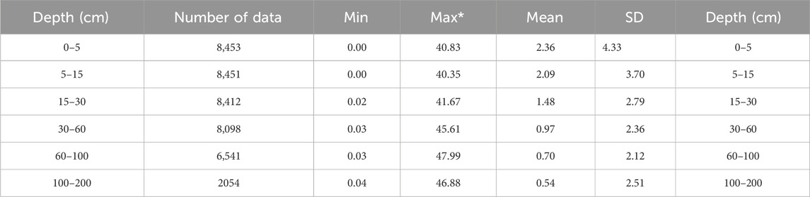
Table 1. Statistical description of soil organic carbon content (% by weight) at multiple depths.

2.2 Environmental covariates

In this study, 134 environmental covariates were considered (Supplementary Table S1), representing factors related to soil and encompassing five major categories, namely, climate, organisms, topography, parent material, and soil types. Climate factors (such as temperature and precipitation) regulate the input and decomposition rates of organic matter by influencing plant growth and microbial activity; biological factors (such as vegetation type and biomass) directly determine the input of organic matter; topographic factors (such as elevation and slope) indirectly affect SOC accumulation by influencing moisture and temperature distribution; parent material factors (such as soil texture and parent rock type) determine the physical and chemical properties of the soil, thereby influencing the stability of organic matter; and soil types and land use practices further reflect the distribution patterns of organic carbon under different soil conditions.

During data processing, covariates with absolute Pearson coefficient values less than 0.05 relative to the target variable are first removed, and then redundant environment covariates with Pearson correlation coefficients greater than 0.8 with other covariates are eliminated. We then iterated over the remaining variables, and 50 covariates were evaluated in batch iterations. Specifically, the covariates were divided into groups of 10; the first iteration started with 10 variables, and 10 additional variables were added in each subsequent iteration until all 50 variables were included. We used the transfer model proposed in this paper to model six different depths of soil profile layers and compared the prediction performance between different subsets according to the RMSE of the predicted results. The results showed that the best model performance was achieved when 37 covariates were included (Table 2). As a result, these 37 environmental covariates were ultimately selected as model inputs (marked with superscript “1” in Supplementary Table S1). To eliminate scale differences among the covariates, the min–max normalization method was used to scale the covariates to a range of 0–1. Normalization not only helps accelerate the convergence speed of the model but also enhances its stability and predictive performance. Through the comprehensive analysis of these covariates, the model can better capture the spatial variability of soil organic carbon, thereby improving prediction accuracy. At the same time, in order to simulate SOC more accurately, the six standard soil layers at different depths mentioned in Section 2.1 are used as input data and are input into the model along with the covariate data.

Table 2

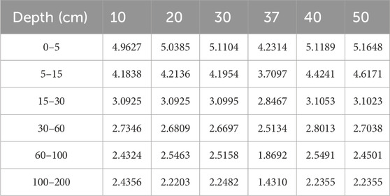
Table 2. RMSE with different variables in six soil layers at different depths.

2.3 Climatic type zoning

China has a vast land area and many different climate types. Different climate types may have different effects on SOC; therefore, in order to more accurately predict SOC of different climate regions, we used the Köppen climate classification, which was developed by German climatologist Wladimir Köppen, to classify the data proposed at the beginning of the 20th century. This system divides the world’s climate into several types based on temperature and precipitation and their annual distribution. The types of climate used in this paper and the results predicted by the model are shown in Section 3.4.

2.4 Benchmark models

In this work, a DL model with CNN structures was developed for SOC prediction. Figure 1 and Supplementary Table S2 illustrate the details of our CNN structures, which were taken as benchmarks for our comparisons. The hyperparameters of the CNN-based model were tuned using soil data from all soil depths. The framework contained three blocks, namely, convolutional, fully connected (FC), and output blocks. The convolutional block consisted of convolutional, max pooling, Swish activation function, batch normalization, and dropout layers. The convolutional block was expected to extract spatial features from environmental covariates; in other words, it was expected to identify representative features of specific soil properties, such as how a peak or a steep slope corresponds to SOC ranges. The fully connected block consisted of fully connected layers, Swish and ReLU activation functions, batch normalization, and dropout layers. The convolutional layer only focused on the neurons in the local field, but the fully connected layer did not. The output of the convolutional block was first flattened and then input to the fully connected block. All the neurons were connected in the fully connected block. The output block was used to predict SOC, which consisted of one fully connected layer. The hyperparameters related to the three blocks and training procedure are listed in Supplementary Table S2.

Figure 1

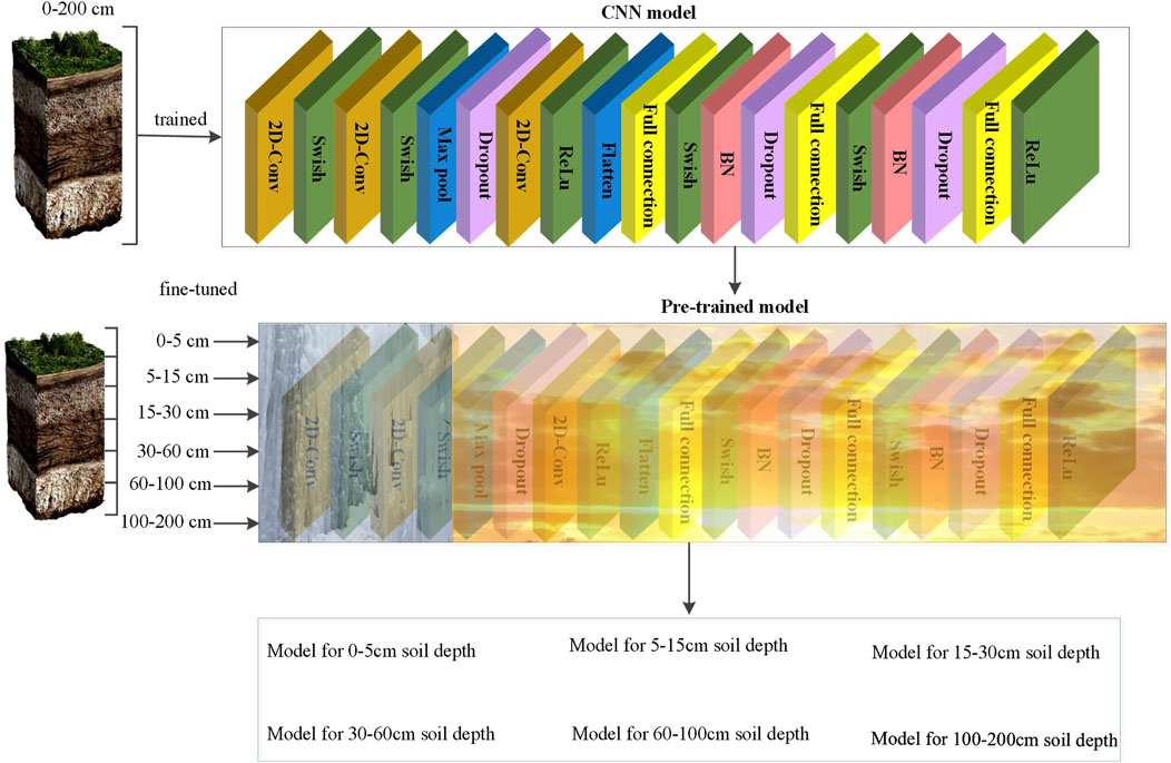
Figure 1. Flowchart for developing the transfer model.

2.5 Transfer model

A CNN model was developed to extract spatial features from multivariate environmental covariates, structured as 2D patches, where each channel represents a specific variable. The architecture includes stacked convolutional layers with Swish activation, MaxPooling, and Dropout, followed by fully connected layers with batch normalization, culminating in a regression output for soil property prediction. The model was initially trained on data spanning all soil depths (0–200 cm) to learn depth-invariant features.

To improve depth-specific performance, a transfer learning strategy was applied. The pre-trained CNN’s early layers were frozen to retain general feature extraction, while the latter layers were fine-tuned for each soil depth interval. This approach allowed adaptation to localized depth patterns while maintaining shared representations. During inference, depth-specific models reuse the common backbone and adjust only the fine-tuned components.

2.6 Multi-task convolutional neural networks model

In this paper, we also employ a multi-task convolutional neural network (MTCNN) as a benchmark model. The structure of the MTCNN model we used is similar to the model structure described by Taghizadeh-Mehrjardi et al. (2020), as shown in Figure 2. It is based on the abovementioned CNN model, which is obtained by modifying it. Unlike the abovementioned CNN, MTCNN has six branches after the flatten layer, each dedicated to predicting SOC at a specific depth. This allows the MTCNN to predict the SOC of six soil layers at the same time. When predicting the SOC of all six layers at the same time, the network shares the structure up to the flatten layer, after which it branches into six independent paths.

Figure 2

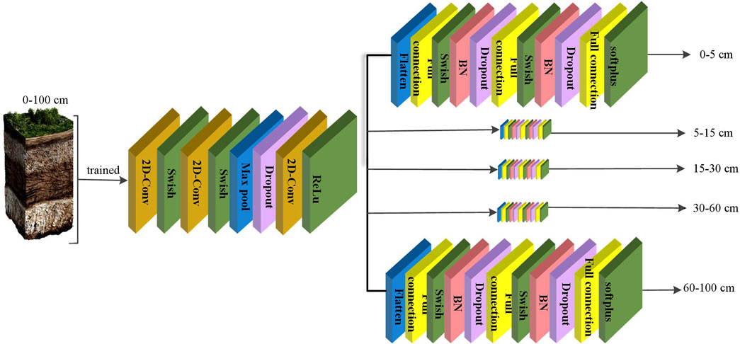
Figure 2. Structural diagram of the MTCNN.

2.7 Evaluation experiments and metrics

During the experiment, we used four models (namely, CNN model, transfer model, RF model, and MTCNN model) for soil mapping. The spatial distribution of the site data used in the experiments is shown in Figure 3. Figure 3A shows the spatial distribution of all 8,453 sites used in the experiments using the CNN model, transfer model, and RF model. Figure 3B shows the distribution of 6,541 sites used in the experiments using the MTCNN model. Because MTCNN is characterized by predicting multiple soil layers of data at the same time, we selected sites with complete data in the first five layers for the experiments, and there were 6,541 eligible sites. We did not pick all six layers with complete data for the experiment because the number of sites with complete data for the six layers was too small; it was only 2,054. The datasets were divided into 90% samples for training and 10% samples for testing. The optimized CNN model with a lower root-mean-squared error was selected based on 10-fold cross-validation with 600 epochs. All predictive models were conducted in Python using the PyTorch and Sklearn tools. RF was used as an additional benchmark for comparison. In the RF model, the hyperparameters max_features and min_samples_leaf were selected from a range [5, 100] with five intervals and [10,100] with 10 intervals, respectively, via the grid search method for preventing the RF model’s over-fitting. Other hyperparameters, such as the number of trees (n_estimators), were not tuned but simply determined based on RF’s own training. Accuracy was evaluated based on five common metrics, namely, the Pearson correlation coefficient (R), R², RMSE, mean absolute error (MAE), and Kling–Gupta efficiency (KGE). R and R² were applied to test the fluctuation pattern and percentage of variance explained by predictive models, respectively. RMSE and MAE denoted the ability to estimate volatility and fluctuation amplitude, respectively. KGE was used to observe the goodness of fit according to the correlation, conditional, and systematic biases. The five metrics were computed as follows:

$RMSE=\sqrt{\frac{{\sum }_{i=1}^N{\left(x_i-y_i\right)}^2}{N}},$

$MAE=\frac{{\sum }_{i=1}^N\left|x_i-y_i\right|}{N},$

$R=\frac{{\sum }_{i=1}^N\left(x_i-\overline{X}\right)\left(y_i-\overline{Y}\right)}{\sqrt{{\displaystyle \sum _{i=1}^n}{\left(x_i-\overline{X}\right)}^2}\sqrt{{\displaystyle \sum _{i=1}^n}{\left(y_i-\overline{Y}\right)}^2}},$

$R^2=1-\frac{{\sum }_{i=1}^N{\left(y_i-x_i\right)}^2}{N{\sum }_{i=1}^N{\left(y_i-\overline{Y}\right)}^2},$

$KGE=1-\sqrt{{\left(R-1\right)}^2+{\left(\alpha -1\right)}^2+{\left(\beta -1\right)}^2},$

where $y_i$ and $x_i$ denote observed and predicted values in the ith soil profile, respectively. $\overline{Y}$ and $\overline{X}$ are the mean values of the observed and predicted values, respectively. $\alpha ={\sigma }_x/{\sigma }_y$,where ${\sigma }_x$ and ${\sigma }_y$ denote the standard deviation of predicted and observed values, respectively. $\beta ={\mu }_x/{\mu }_y$,where ${\mu }_x$ and ${\mu }_y$ represent the mean of predicted and observed values, respectively.

Figure 3

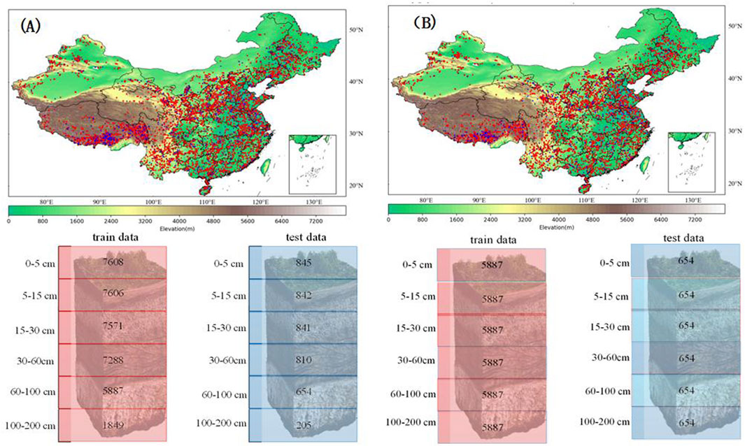
Figure 3. Study area in China and the spatial distribution of soil profiles over the study area. (A) CNN model, RF model, and the transfer model experiment setting. (B) MTCNN model experiment setting. The red points are for training, the blue points are for testing, and the number at each depth are the number of observations.

3 Results

3.1 Evaluation of the productive models

We show the distribution of values for the test set of the four models in a scatterplot to visualize the correlation between the predicted and observed values. The scatter plots between predictions and observations from the whole soil profiles are shown in Figure 4. Figure 4 shows that the transfer model, CNN, and RF achieve relatively accurate prediction results compared to the MTCNN, which has significantly worse prediction results. The transfer model could achieve better performance than other models in mapping SOC at unseen profiles, which had reductions of 9.38% and 13.70% for the RF model and 2% and 9.12% for the CNN model, according to the RMSE and MAE metrics and yielded higher R² (0.374), R (0.618), and KGE (0.373). Meanwhile, similar to previous studies (Sanderman et al., 2018; Sothe et al., 2022; Keskin et al. (2019)), lower SOC values were slightly overestimated and higher SOC values were generally underestimated. To overcome this problem, we also applied the logarithmic transformation before the training process, as suggested by other studies (Guevara et al., 2020; Hengl et al., 2017), but it had little impact on the model performance. Hence, the original SOC values were retained in our study.

Figure 4

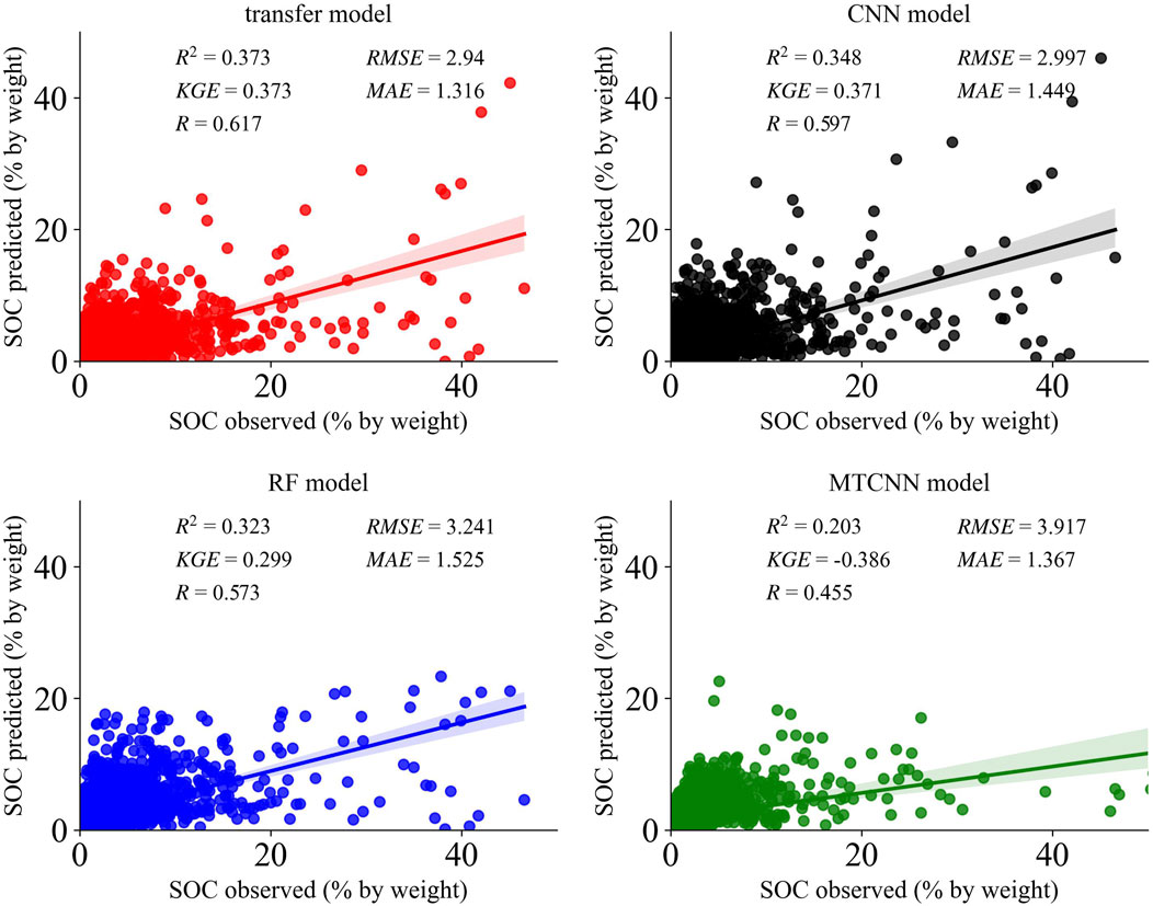
Figure 4. Comparisons between the observed and predicted SOC values from all soil depths.

3.2 Comparison of the productive model at each soil depth

Due to the characteristics of the MTCNN model, we selected a different test set than the other three models used in the experiments with the MTCNN in order to ensure that there are no missing values in the first five layers of each test site. Therefore, we discuss the MTCNN separately from the other three models.

As an additional visual analysis, the statistical results of three models (transfer model, CNN model, and RF model) with all soil depths and the best-performing figure are illustrated in Supplementary Table S3; Figure 5. In most cases, the transfer model showed superior performance compared to other models. The RF model had lower RMSE at 30–60 cm soil depth. Meanwhile, according to the R² (less than 0.1) and KGE (negative scores) metrics, poor performance was achieved by all models from 30 to 200 cm soil depths. Figure 6 shows the predicted maps of SOC using the proposed transfer model. In general, the spatial distribution of SOC was similar for all soil depths. It could be observed that SOC in northeast China, southwest China, and some regions of northwest China was relatively higher than that in other regions. Meanwhile, SOC across China started to decrease as the soil depth increased. The distribution of the predicted SOC maps using the proposed transfer model was also consistent with the findings of a recent study (Liu et al., 2022). Overall, the transfer model outperformed the state-of-the-art models (RF and CNN) in terms of statistical metrics and provided a reasonable spatial pattern for SOC mapping.

Figure 5

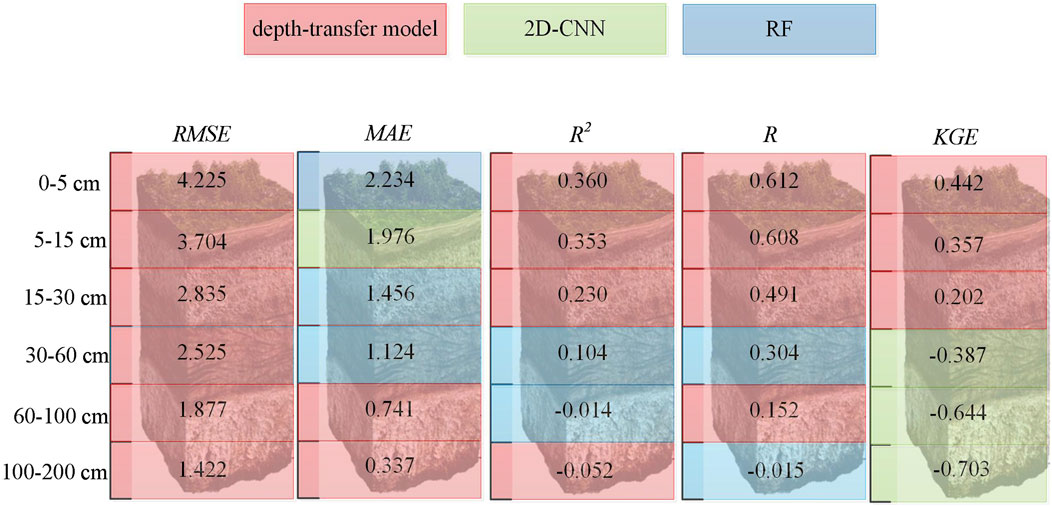
Figure 5. Best-performing model at each depth.

Figure 6

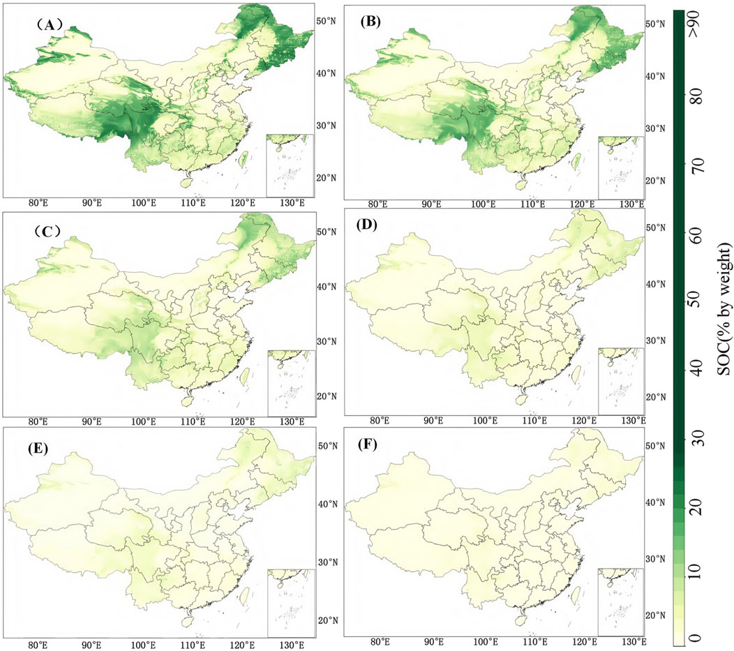
Figure 6. Spatial distribution of soil organic carbon predicted by the transfer model at (A) 0–5 cm, (B) 5–15 cm, (C) 15–30 cm, (D) 30–60 cm, (E) 60–100 cm, and (F) 100–200 cm.

3.3 Predictive performance of the MTCNN model

Figure 7 shows the spatial distribution of soil organic carbon predicted by the transfer and MTCNN models. The overall spatial distribution of soil organic carbon predicted by the transfer model is consistent with the results of Liu et al. (2022), so we believe that the results of the transfer model are more credible. Compared with the results of the transfer model, the overall spatial distribution of the results of the MTCNN model is consistent with the results of the transfer model, but there is a big gap in the details. For example, in places with high soil carbon content, such as the Tibetan Plateau and northeast China, the prediction results of the MTCNN model are significantly lower. The statistical results of the MTCNN model with all soil depths are illustrated in Supplementary Table S4.

Figure 7

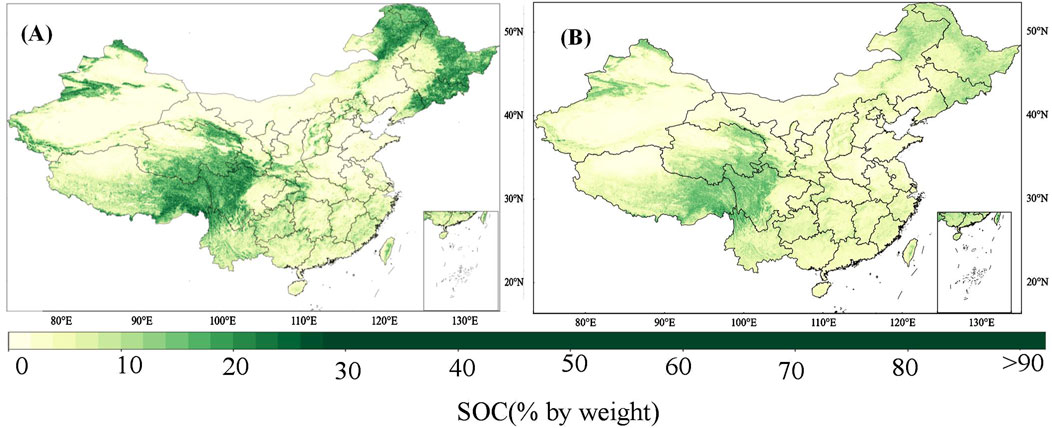
Figure 7. Spatial distribution of soil organic carbon predicted by the transfer model (A) and MTCNN model (B) at 0–5 cm.

3.4 Modeling of different climate zones

Figure 8 presents the RMSE performance of the CNN model and the proposed transfer learning model across different Köppen climate zones. The RMSE values of the transfer model are generally closer to those of the CNN model across all climate zones. Notably, the transfer model shows more substantial improvements in tropical and dry climates, suggesting that transfer learning can effectively leverage knowledge from other regions to enhance prediction performance in areas with limited or heterogeneous data.

Figure 8

Figure 8. Prediction effect of the CNN model and the transfer model in different climate regions.

However, in polar climates, both models still exhibit relatively high prediction errors. This may be attributed to the inherent challenges of modeling SOC in such regions. Existing studies have shown that SOC sequestration is closely related to soil microbial activity (Dubeux et al., 2024); large animals, such as earthworms, ants, and termites, form burrows, where SOC accumulates and transfers from the top layer (Nielsen and Hole, 1964; Lorenz and Lal, 2005), which may be significantly inhibited under extremely low temperatures. As a result, conventional environmental covariates—such as temperature and vegetation indices—may lack representativeness and explanatory power in polar environments, thus limiting the overall model performance.

3.5 Effect of the transfer model on different properties

To further illustrate the effectiveness of the transfer model, we simulated another soil texture property—clay—alongside SOC for different soil layers. The method of filtering the data is the same as described in Section 2.2; after the final iteration, 37 covariates related to clay and the corresponding soil layer are selected as inputs, and some of the noisy data are removed. Figure 9 shows the comparison of the performance (measured as RMSE) of the models with and without transfer learning for predicting SOC and clay at different soil depths. Compared to the model without transfer, the transfer model reduced RMSE values substantially when predicting SOC, particularly at shallow soil layers (layers 1–3), indicating that the transfer method captures the spatial distribution of SOC more effectively, thus enhancing the model’s generalization capability. Additionally, the transfer model also demonstrated noticeable improvements in predicting the clay content, especially in soil layers 1, 3, and 5. This also shows that the transfer model proposed in this paper can achieve more accurate predictions.

Figure 9

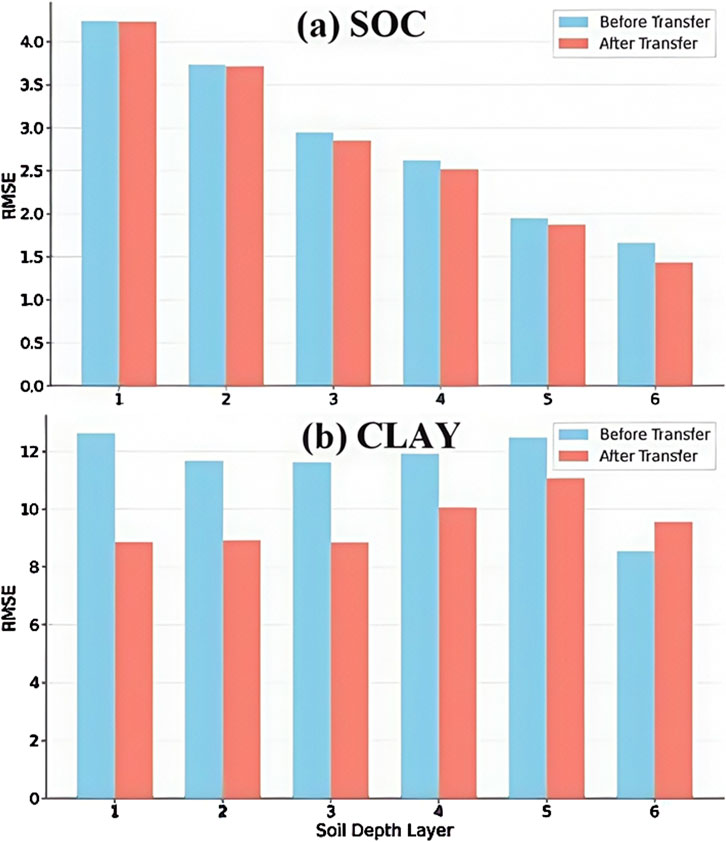
Figure 9. The effects of the transfer model and the non-transfer model on different variables, where (a) represents the effects of the two models in simulating SOC and (b) represents the effects of the two models in simulating CLAY.

3.6 Effect of the model at different SOC levels

Figure 10 shows the comparison of the probability density distributions of the predicted and observed SOC values under different SOC levels for four models, namely, the transfer model, CNN, MTCNN, and RF. It is evident that the transfer model yields a predicted distribution that most closely aligns with the true distribution in the high-density region (0–2.5), with remarkable consistency in both peak position and overall curve shape. This suggests that the transfer model possesses a stronger capability in learning SOC distribution characteristics and exhibits superior generalization performance. In contrast, the CNN and MTCNN show noticeable shifts in the main peak positions, indicating systematic errors in the core SOC range. In other regions, the predictions of the transfer model also remain closer to the observed values. Moreover, the predicted mean of the transfer model nearly coincides with the true mean, highlighting its advantage in controlling overall bias. These findings demonstrate that the transfer model not only outperforms the other models in fitting the overall distribution but also more accurately captures the distribution of low SOC regions, which constitute the majority of the dataset.

Figure 10

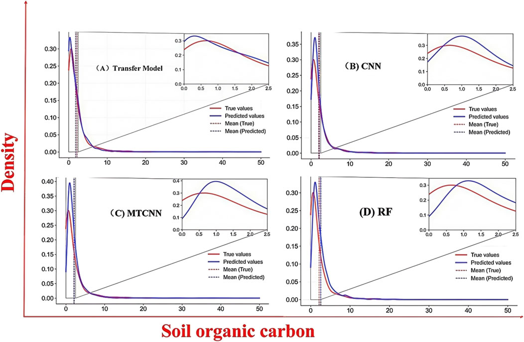
Figure 10. The density curves of models with different SOC contents, (A–D) represent the density curves of four models, namely, Transfer Model, CNN, MTCNN and RF.

4 Discussion

4.1 Transfer learning’s impact on subsoil modeling

The results (Figure 6; Supplementary Tables S3, S4) show that the performance of all models decreased as the soil depth increased. This was also consistent with most previous studies (Akpa et al., 2016; Kempen et al., 2011; Mulder et al., 2016; Padarian et al., 2017). The reason may be that the used covariates depict the variations in the surface soil layer and are not sensitive to the variations in subsoil. Another reason may be that there are few samples at deeper layers, especially for the deepest layer (100–200 cm). However, we found that for deeper soil layers, the transfer model improved more significantly than the CNN model. We could see that R² values achieved by the transfer model were 0.230, −0.041, and −0.052, compared to 0.175, −0.131, and −0.411 (CNN) at 15–30, 60–100, and 100–200 cm soil depths, respectively. This enormous improvement should be attributed to the adjacent layers. Since we used all six layers of data to initialize the transfer model, the model contains the information on the adjacent soil layers.

4.2 Comparisons of predictive models in different regions

This section aimed at analyzing the performance of different models in different regions in China. Hence, the relative bias of the tested profiles is represented in Figures 11, 12. Figure 11 shows the relative bias of all models at 0–5 cm soil depth. From Figure 8, we can see that a larger relative bias existed in northeast, northern Xinjiang, and southern Tibet for all models, and a smaller relative bias appeared in south China. Furthermore, the relative bias in some regions started to get smaller as the soil depth increased, such as in Jilin province and Tibet (not shown in figures). In order to reduce the relative bias in some specific regions, such as east and west Tibet, we tried to perform a new testing method, applying different covariates (adding 43 new covariates selected by RF with a superscript “2” in Table 2), and the results are shown in Figure 12. Even though the overall performance of the new model was no better than that of the original model, the relative bias began to decrease in the rectangular regions. This indicates that the relative bias in local regions can be reduced by exploring more useful covariates. The reason may be that different covariates had different sensitivities to soil data in different regions (Wang et al., 2021).

Figure 11

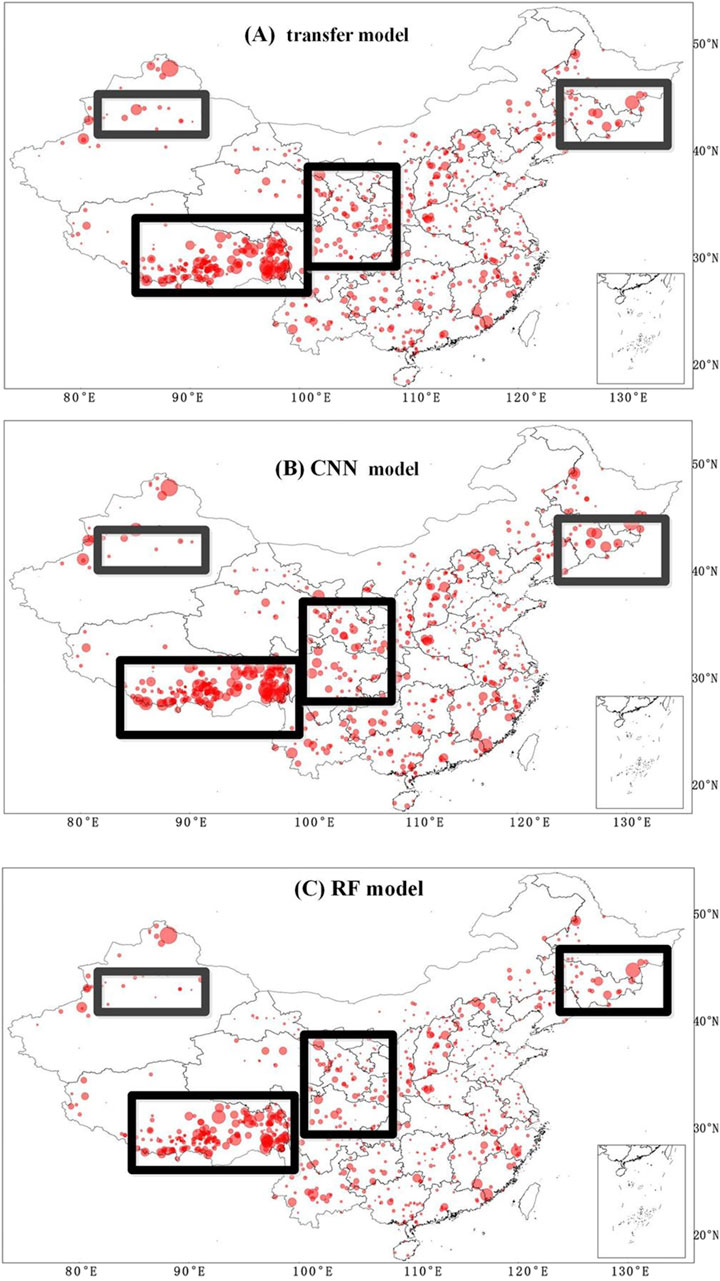
Figure 11. Relative bias at 0–5 cm soil depth for the transfer model, CNN model, and RF model. In the figure, (A) stands for transfer mode, (B) stands for CNN and (C) stands for RF. The size of the three geometric figures indicates the relative bias, which is computed as follows: $y=\left(x-\mathit{max}\left(x\right)\right)$∗10³, where $y$ is the relative bias, $x$ is the predictions, and $\mathit{max}\left(x\right)$ is the maximum of predictions.

Figure 12

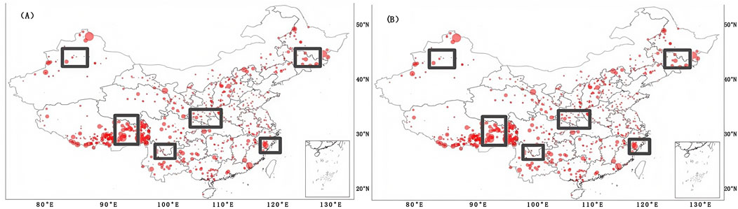
Figure 12. Relative bias of the transfer model with different covariates with (A) the selected 37 covariates in this study, and (B) after adding an additional 43 covariates selected by RF.

4.3 Evaluations of frozen layers in the deep learning model

DL-based models have been successfully applied in digital soil mapping. Different layers in DL models presented different roles. Hence, we tried to freeze the different layers for evaluating the performance of the transfer model. Supplementary Figure S1 illustrates the performance of the transfer model when fine-tuning different layers, where ID represents the identification number of the layers, and layers denote their names in the model. For example, when ID is “1,” the layer denotes the ‘first convolutional layer’; when ID is “2,” layers denote the “second convolutional layer”; when ID is “3,” layers denote the “third convolutional layer”; when ID is “4,” layers denote the “first fully connected layer”; when ID is “5,” layers denote the “second fully connected layer,” and when ID was “6,” layers denote the ‘third fully connected layer.’ In this process, all layers before and including the selected layer were frozen, and the remaining layers were fine-tuned. According to Supplementary Figure S1, although the best performance was not obtained when the convolutional block was frozen, it could achieve the relatively excellent performance across to all metrics. Hence, the convolutional block (the first two convolution layers) was chosen to be frozen in our experiment. The reason is discussed by comparing the practice of image processing and digital soil mapping as follows. Specifically, for CNN-based models in image processing, each layer held the hierarchical nature of the features in the model. For instance, the visualization of features in a fully trained 5-layered model denoted that the initial layers usually described the macroscopic properties of objects (e.g., edge/color conjunctions and mesh patterns) and the last layers could describe the minor and detailed features of objects (e.g., dog faces and bird’s legs). Hence, in our testing, the initial layers may represent the macroscopic conditions of soil-forming factors, which denoted the features between environmental covariates and soil profiles, and we could freeze the convolutional block to save the general features learned from all soil layers. The remaining layers may represent the detailed conditions of soil-forming factors, which denoted the features between environmental covariates and each soil layer, and we could fine-tune them to establish a specific model from a “big knowledge base” (the general features learned from all soil layers) for localizing to a specific soil depth, which could help the model to improve predictive performance.

4.4 Analysis of predictive models with important covariates

As shown in Figure 13, we investigated the predictions of the transfer model and observed SOC values along with most related covariates (mean long-term surface temperature in June/July) and land surface elevation (DEM). For three representative soil depths in training sets, it can be observed that most soil data with relatively low SOC (less than 7%) were located in the blue rectangle, where the mean long-term surface temperature in June/July was more than 25°C, while the values of SOC more than 10% are usually distributed in regions that had low mean long-term surface temperature in June/July and higher elevations (more than 3,000 m). Meanwhile, in the topsoil from 0 to 30 cm soil depth, the soil with high SOC had a larger quantity than other soil depths, which is denoted in a red rectangle in Figure 10. This resulted in the predictions having similar distributions.

Figure 13

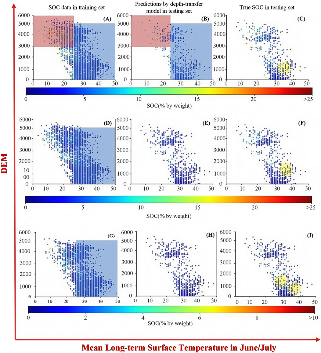
Figure 13. Performance of the transfer model for fine-tuning the different layers. (A–C) 0–5 cm, (D–F) 15–30 cm, and (G–I) 60–100 cm soil depths. The first column denotes SOC data in the training set, the second column shows predictions by the transfer model in the testing set, and the last column represents the observed SOC in the testing set.

With SOC in the training sets (red and blue rectangles in the second column), however, two cases in Figure 13 are worth noting. The first is that the proportion of relatively higher SOC values gradually decreased as the soil depth increased; this made predicting higher SOC values challenging, and poor predictions for higher SOC were noticeable at soil depths ranging from 30 to 200 cm. The second case is that some individual cases from the observed SOC in the testing sets were always unpredictable (yellow circle regions). Several reasons may cause these two problems, and the major one among them may be the unbalanced nature of the SOC dataset, which made individual case prediction challenging. The cost-sensitive-based DL model (Telikani et al., 2022) could be explored in the future and may penalize prediction errors for the abovementioned cases.

4.5 Effect of covariates on SOC

In this study, climate, soil types, and texture-related environmental covariates were used as model inputs. Previous research has demonstrated that these factors have a significant impact on SOC content, which is also reflected in several experimental results of this study. In terms of climatic variables, increases in precipitation and clay content promote SOC accumulation, while higher temperatures accelerate its decomposition (Jobbágy and Jackson, 2000; Singh et al., 2017), with deep-layer SOC being more sensitive to temperature changes (Li et al., 2020b). These findings help explain the higher prediction errors observed in warm and humid regions and the superior performance of the transfer learning model in deeper soil layers (60–200 cm).

Regarding soil texture, the proportions of silt and clay play a crucial role in SOC stabilization and vary significantly with depth (Bauer et al., 1987; Button et al., 2022; Six et al., 2000; Chivenge et al., 2007). This supports our variable iteration experiments, which showed improved model performance when texture-related variables were included, and it also validates the use of soil depth as an input covariate.

Furthermore, SOC distribution is highly uneven across soil profiles, with up to 80% of total SOC stored below 90 cm depth (Jobbágy and Jackson, 2000; Rolando et al., 2021; Gross and Harrison, 2019). Therefore, modeling full-profile information using transfer learning enhances the model’s ability to capture deep SOC patterns, demonstrating that incorporating all soil depths and applying transfer learning effectively improves the overall prediction accuracy.

5 Conclusion

With the development of computational power in recent years, deep learning techniques have begun to be widely used across various industries, including the field of soil mapping. Although deep learning models have been successfully applied in digital soil mapping, localizing to a specific soil depth for deep learning-based models is challenging as the training method using gradient descent may not directly relate to the specific depth model. We designed a transfer learning method based on the CNN model to improve the specific soil depth model. Without relying on external data, we developed a transfer learning scheme according to the characteristics of soil data, which makes more effective use of limited data. This transfer method uses information from all soil depths to more accurately predict SOC at each specific depth. This method outperforms state-of-the-art models (RF, CNN, and MTCNN) in terms of statistical metrics for SOC mapping. We recommend freezing the first few layers in the transfer deep learning model during fine-tuning.

Meanwhile, according to comparisons of predictive models in different regions, the larger relative bias existed in the east and west parts of Tibet, and more useful covariates should be explored due to the different impacts of covariates on soil data in different regions. Through analysis of predictive models with important covariates, some individual cases were always found to be unpredictable, and the cost-sensitive-based DL models were advocated to be designed for penalizing prediction errors of individual cases.

Data availability statement

The original contributions presented in the study are included in the article/Supplementary Material; further inquiries can be directed to the corresponding author.

Author contributions

JH: conceptualization, data curation, funding acquisition, investigation, methodology, project administration, validation, visualization, and writing – original draft. MW: conceptualization, supervision, validation, and writing – original draft. YQ: software and writing – review and editing. XL: validation and writing – review and editing. XC: formal analysis and writing – review and editing. JW: resources and writing – review and editing. JZ: formal analysis and writing – review and editing. QL: writing – review and editing.

Funding

The author(s) declare that financial support was received for the research and/or publication of this article. This work was supported by the Jilin Provincial Science and Technology Development Plan Project under grant number 20230101370JCJC.

Acknowledgments

The authors would like to thank all the colleagues and collaborators who provided valuable feedback and support throughout the research process.

Conflict of interest

The authors declare that the research was conducted in the absence of any commercial or financial relationships that could be construed as a potential conflict of interest.

Generative AI statement

The author(s) declare that no Generative AI was used in the creation of this manuscript.

Publisher’s note

All claims expressed in this article are solely those of the authors and do not necessarily represent those of their affiliated organizations, or those of the publisher, the editors and the reviewers. Any product that may be evaluated in this article, or claim that may be made by its manufacturer, is not guaranteed or endorsed by the publisher.

Supplementary material

The Supplementary Material for this article can be found online at: https://www.frontiersin.org/articles/10.3389/fenvs.2025.1580085/full#supplementary-material

References

Akpa, S., Odeh, I., Bishop, T., Hartemink, A. E., and Amapu, I. Y. (2016). Total soil organic carbon and carbon sequestration potential in Nigeria. Geoderma 271, 202–215. doi:10.1016/j.geoderma.2016.02.021

CrossRef Full Text | Google Scholar

Araujo, A., Leite, L., Iwata, B., Junior, M., and Figueiredo, M. (2012). Microbiological process in agroforestry systems. A Rev. Agron. Sustain. Dev. 32 (1), 215–216. doi:10.1007/s13593-011-0026-0

CrossRef Full Text | Google Scholar

Bauer, A., Cole, C. V., and Black, A. L. (1987). Soil property comparisons in virgin grasslands between grazed and nongrazed management systems. Soil Sci. Soc. Am. J. 51, 176–182. doi:10.2136/sssaj1987.03615995005100010037x

CrossRef Full Text | Google Scholar

Bian, Z., Guo, X., Wang, S., Zhuang, Q., Jin, X., Wang, Q., et al. (2019). Applying statistical methods to map soil organic carbon of agricultural lands in northeastern coastal areas of China. Archives Agron. and Soil Sci. 66 (4), 532–544. doi:10.1080/03650340.2019.1626983

CrossRef Full Text | Google Scholar

Blanco, C. G., Gomez, V. B., Crespo, P., and Lie?, M. (2018). Spatial prediction of soil water retention in a Páramo landscape: methodological insight into machine learning using random forest. Geoderma 316, 100–114. doi:10.1016/j.geoderma.2017.12.002

CrossRef Full Text | Google Scholar

Button, E. S., Pett-Ridge, J., Murphy, D. V., Kuzyakov, Y., Chadwick, D. R., and Jones, D. L. (2022). Deep-C storage: biological, chemical and physical strategies to enhance carbon stocks in agricultural subsoils. Soil Biol. Biochem. 170, 108697. 0038-0717. doi:10.1016/j.soilbio.2022.108697

CrossRef Full Text | Google Scholar

Chivenge, P., Murwira, H. K., Giller, K. E., Mapfumo, P., and Six, J. (2007). Long-term impact of reduced tillage and residue management on soil carbon stabilization: implications for conservation agriculture on contrasting soils. Soil Tillage Res. 94 (2), 328–337. ISSN 0167-1987. doi:10.1016/j.still.2006.08.006

CrossRef Full Text | Google Scholar

Dobarco, M. R., McBratney, A., Minasny, B., and Malone, B. (2021). A modelling framework for pedogenon mapping. Geoderma 393, 115012. doi:10.1016/j.geoderma.2021.115012

CrossRef Full Text | Google Scholar

Dubeux, J. C. B., Lira Junior, M. A., Simili, F. F., Bretas, I. L., Trumpp, K. R., Bizzuti, B. E., et al. (2024). Deep soil organic carbon: a review. United Kingdom: CABI Reviews. doi:10.1079/cabireviews.2024.0024

CrossRef Full Text | Google Scholar

Gross, C. D., and Harrison, R. B. (2019). The case for digging deeper: soil organic carbon storage, dynamics, and controls in our changing world. Soil Syst. 3, 28. doi:10.3390/soilsystems3020028

CrossRef Full Text | Google Scholar

Guevara, M., Arroyo, C., Brunsell, N., Cruz, C. O., Domke, G., Equihua, J., et al. (2020). Soil organic carbon across mexico and the conterminous United States (1991–2010). Glob. Biogeochem. Cycles 34, e2019GB006219. doi:10.1029/2019GB006219

CrossRef Full Text | Google Scholar

Han, L., Sun, K., Jin, J., and Xing, B. (2016). Some concepts of soil organic carbon characteristics and mineral interaction from a review of literature. Soil Biol. Biochem. 94 (2016), 107–121. ISSN 0038-0717. doi:10.1016/j.soilbio.2015.11.023

CrossRef Full Text | Google Scholar

Hengl, T., Jesus, J., Heuvelink, G., Gonzalez, M. R., Kempen, B., Blagotić, A., et al. (2017). SoilGrids250m: global gridded soil information based on machine learning. PLoS ONE 12 (2), e0169748. doi:10.1371/journal.pone.0169748

PubMed Abstract | CrossRef Full Text | Google Scholar

Hengl, T., Miller, M., Krian, J., Shepherd, K. D., Sila, A., Kilibarda, M., et al. (2021). African soil properties and nutrients mapped at 30m spatial resolution using two-scale ensemble machine learning. Sci. Rep. 11, 6130. doi:10.1038/s41598-021-85639-y

PubMed Abstract | CrossRef Full Text | Google Scholar

Jobbágy, E. G., and Jackson, R. B. (2000). The vertical distribution of soil organic carbon and its relation to climate and vegetation. Ecol. Appl. 10, 423–436. doi:10.1890/1051-0761(2000)010[0423:TVDOSO]2.0.CO;2

CrossRef Full Text | Google Scholar

Kempen, B., Brus, D. J., and Stoorvogel, J. J. (2011). Three-dimensional mapping of soil organic matter content using soil type-specific depth functions. Geoderma 162 (1-2), 107–123. doi:10.1016/j.geoderma.2011.01.010

CrossRef Full Text | Google Scholar

Keskin, H., Grunwald, S., and Harris, W. G. (2019). Digital mapping of soil carbon fractions with machine learning. Geoderma 339, 40–58. doi:10.1016/j.geoderma.2018.12.037

CrossRef Full Text | Google Scholar

Kheir, R. B., Greve, M. H., Bocher, P. K., Greve, M. B., Larsen, R., and Mccloy, K. (2010). Predictive mapping of soil organic carbon in wet cultivated lands using classification-tree based models: the case study of Denmark. J. Environ. Manag. 91 (5), 1150–1160. doi:10.1016/j.jenvman.2010.01.001

CrossRef Full Text | Google Scholar

Kim, J., and Grunwald, S. (2016). Assessment of carbon stocks in the topsoil using random forest and remote sensing images. J. Environ. Qual. 45 (6), 1910–1918. doi:10.2134/jeq2016.03.0076

PubMed Abstract | CrossRef Full Text | Google Scholar

Lal, R. (2004). Soil carbon sequestration impacts on global climate change and food security. Science 304 (5677), 1623–1627. doi:10.1126/science.1097396

PubMed Abstract | CrossRef Full Text | Google Scholar

Lausch, A., Baade, J., Bannehr, L., Borg, E., Schaepman, M. E., Chabrilliat, S., et al. (2019). Linking remote sensing and geodiversity and their traits relevant to biodiversity—Part I: soil characteristics. Remote Sens. 11 (20), 2356. doi:10.3390/rs11202356

CrossRef Full Text | Google Scholar

Li, J., Pei, J., Pendall, E., Reich, P. B., Noh, N. J., Li, B., et al. (2020b). Rising temperature may trigger deep soil carbon loss across forest ecosystems. Adv. Sci. 7, 2001242. doi:10.1002/advs.202001242

PubMed Abstract | CrossRef Full Text | Google Scholar

Li, Q., Hao, H., Zhao, Y., Geng, Q., Liu, G., Zhang, Y., et al. (2020a). GANs-LSTM model for soil temperature estimation from meteorological: a new approach. IEEE Access 8 (2020), 59427–59443. doi:10.1109/ACCESS.2020.2982996

CrossRef Full Text | Google Scholar

Li, Q., Li, Z., Shangguan, W., Wang, X., Li, L., and Yu, F. (2022a). Improving soil moisture prediction using a novel encoder-decoder model with residual learning. Comput. Electron. Agric. 195, 106816. doi:10.1016/j.compag.2022.106816

CrossRef Full Text | Google Scholar

Li, Q., Zhu, Y., Shangguan, W., Wang, X., Li, L., and Yu, F. (2022b). An attention-aware LSTM model for soil moisture and soil temperature prediction. Geoderma 409, 115651. doi:10.1016/j.geoderma.2021.115651

CrossRef Full Text | Google Scholar

Liu, F., Wu, H., Zhao, Y., Li, D., Yang, J.-L., Song, X., et al. (2022). Mapping high resolution national soil information grids of China. Sci. Bull. 67 (3), 328–340. doi:10.1016/j.scib.2021.10.013

PubMed Abstract | CrossRef Full Text | Google Scholar

Lorenz, K., and Lal, R. (2005). The depth distribution of soil organic carbon in relation to land use and management and the potential of carbon sequestration in subsoil horizons, Adv. Agron. 88, 35–66. doi:10.1016/S0065-2113(05)88002-2

CrossRef Full Text | Google Scholar

Ma, Y., Minasny, B., McBratney, A., Poggio, L., and Fajardo, M. (2021). Predicting soil properties in 3D: should depth be a covariate? Geoderma 383, 114794. doi:10.1016/j.geoderma.2020.114794

CrossRef Full Text | Google Scholar

Mulder, V. L., Lacoste, M., Richer-De-Forges, A. C., and Arrouays, D. (2016). GlobalSoilMap France: high-resolution spatial modelling the soils of France up to two meter depth. Sci. Total Environ. 573 (dec.15), 1352–1369. doi:10.1016/j.scitotenv.2016.07.066

PubMed Abstract | CrossRef Full Text | Google Scholar

Nielsen, G. A., and Hole, F. D. (1964). Earthworms and the development of coprogenous A1 horizons in forest soils of Wisconsin. Soil Sci. Soc. Am. J. 28, 426–430. doi:10.2136/sssaj1964.03615995002800030037x

CrossRef Full Text | Google Scholar

Padarian, J., Minasny, B., and Mcbratney, A. B. (2017). Chile and the Chilean soil grid: a contribution to GlobalSoilMap. Geoderma Reg. 9, 17–28. doi:10.1016/j.geodrs.2016.12.001

CrossRef Full Text | Google Scholar

Piikki, K., Söderström, M., and Stenberg, B. (2013). Sensor data fusion for topsoil clay mapping. Geoderma 199, 106–116. doi:10.1016/j.geoderma.2012.10.007

CrossRef Full Text | Google Scholar

Rolando, J. L., Dubeux, J. C. B., de Souza, T. C., Mackowiak, C., Wright, D., George, S., et al. (2021). Organic carbon is mostly stored in deep soil and only affected by land use in its superficial layers: a case study. Agrosyst Geosci. Environ. 4, e20135. doi:10.1002/agg2.20135

CrossRef Full Text | Google Scholar

Sanderman, J., Hengl, T., Fiske, G., Solvik, K., Adame, M. F., Benson, L., et al. (2018). A global map of mangrove forest soil carbon at 30m spatial resolution. Environ. Res. Lett. 13, 055002. doi:10.1088/1748-9326/aabe1c

CrossRef Full Text | Google Scholar

Shen, Z., Ramirez-Lopez, L., Behrens, T., Cui, L., Zhang, M., Walden, L., et al. (2022). Deep transfer learning of global spectra for local soil carbon monitoring. ISPRS J. Photogrammetry Remote Sens. 188 (2022), 190–200. doi:10.1016/j.isprsjprs.2022.04.009

CrossRef Full Text | Google Scholar

Singh, M., Sarkar, B., Biswas, B., Bolan, N. S., and Churchman, G. J. (2017). Relationship between soil clay mineralogy and carbon protection capacity as influenced by temperature and moisture. Soil Biol. Biochem. 109, 95–106. ISSN 0038-0717. doi:10.1016/j.soilbio.2017.02.003

CrossRef Full Text | Google Scholar

Six, J., Elliott, E. T., and Paustian, K. (2000). Soil macroaggregate turnover and microaggregate formation: a mechanism for C sequestration under no-tillage agriculture. Soil Biol. Biochem. 32 (14), 2099–2103. ISSN 0038-0717. doi:10.1016/S0038-0717(00)00179-6

CrossRef Full Text | Google Scholar

Sothe, C., Gonsamo, A., Arabian, J., and Snider, J. (2022). Large scale mapping of soil organic carbon concentration with 3D machine learning and satellite observations. Geoderma 405, 115402. doi:10.1016/j.geoderma.2021.115402

CrossRef Full Text | Google Scholar

Sreenivas, K., Sujatha, G., Sudhir, K., Kiran, D. V., Dadhwal, V. K., Ravisankar, T., et al. (2014). Spatial assessment of soil organic carbon density through random Forests based imputation. J. Indian Soc. Remote Sens. 42 (3), 577–587. doi:10.1007/s12524-013-0332-x

CrossRef Full Text | Google Scholar

Taghizadeh-Mehrjardi, R., Mahdianpari, M., Mohammadimanesh, F., Behrens, T., Schmidt, K., Scholten, T., et al. (2020). Multi-task convolutional neural networks outperformed random forest for mapping soil particle size fractions in central Iran. Geoderma 378, 114552. doi:10.1016/j.geoderma.2020.114552

CrossRef Full Text | Google Scholar

Telikani, A., Gandomi, A. H., Choo, K.-K. R., and Shen, J. (2022). A cost-sensitive deep learning-based approach for network traffic classification. IEEE Trans. Netw. Serv. Manag. 19 (1), 661–670. doi:10.1109/TNSM.2021.3112283

CrossRef Full Text | Google Scholar

Wang, Y., Mao, J., Jin, M., Hoffman, F. M., Dai, Y., Wullschleger, S. D., et al. (2021). Development of observation-based global multi-layer soil moisture products for 1970 to 2016. Earth Syst. Sci. Data 13 (9), 4385–4405. doi:10.5194/essd-13-4385-2021

CrossRef Full Text | Google Scholar

Wiesmeier, M., Barthold, F., Blank, B., and Kögel-Knabner, I. (2011). Digital mapping of soil organic matter stocks using Random Forest modeling in a semi-arid steppe ecosystem. Plant and Soil 340 (s1-2), 7–24. doi:10.1007/s11104-010-0425-z

CrossRef Full Text | Google Scholar

Wu, W., Li, A. D., He, X. H., Ma, R., and Lv, J. K. (2018). A comparison of support vector machines, artificial neural network and classification tree for identifying soil texture classes in southwest China. Comput. and Electron. Agric. 144, 86–93. doi:10.1016/j.compag.2017.11.037

CrossRef Full Text | Google Scholar

Yang, J., Wang, X., Wang, R., and Wang, H. (2020). Combination of convolutional neural networks and recurrent neural networks for predicting soil properties using vis–NIR spectroscopy. Geoderma 380, 114616. doi:10.1016/j.geoderma.2020.114616

CrossRef Full Text | Google Scholar

Yang, L., Cai, Y., Zhang, L., Guo, M., and Zhou, C. (2021). A deep learning method to predict soil organic carbon content at a regional scale using satellite-based phenology variables. Int. J. Appl. Earth Observation Geoinformation 102 (6), 102428. doi:10.1016/j.jag.2021.102428

CrossRef Full Text | Google Scholar

Zhang, G., and Gong, Z. (2012). Soil survey laboratory methods. Beijing: Science Press.

Google Scholar

Zhang, Y., Sui, B., Shen, H., and Ouyang, L. (2019). Mapping stocks of soil total nitrogen using remote sensing data: a comparison of random forest models with different predictors. Comput. Electron. Agric. 160, 23–30. doi:10.1016/j.compag.2019.03.015

CrossRef Full Text | Google Scholar

Zhao, Z., Chow, T. L., Rees, H. W., Yang, Q., Xing, Z., and Meng, F. R. (2009). Predict soil texture distributions using an artificial neural network model. Comput. and Electron. Agric. 65 (1), 36–48. doi:10.1016/j.compag.2008.07.008

CrossRef Full Text | Google Scholar