Advanced GIS-based modeling for flood hazards mapping in urban semi-arid regions: insights from Beni Mellal, Morocco

Floods are among the most destructive natural disasters, threatening people, the economy and cultural heritage. In Beni-Mellal, mountainous topography accentuates this risk by promoting the rapid flow of water to low-lying areas, where it accumulates more easily. This study maps the flood risk using three statistical methods: Information Value (IV), Weighting Factor (WF) and Weight of Evidence (WoE). A detailed database was built, combining an inventory of floods and key environmental variables, such as slope, proximity to rivers, land use and the Topographic Humidity Index (TWI). The database was built on pre-processed and standardized Sentinel-2 and Landsat 8 satellite images, as well as geological and soil maps, ensuring full coverage and high-definition resolution of 12.5 m to ensure optimal spatial accuracy. The results show that 4.4%–13.6% of the region is classified as very high risk, 13.8%–31.1% at high risk, and 24.5%–31.2% at moderate risk, with increased vulnerability in the southern areas, where land slope and occupation play a major role. The evaluation of model performance reveals that WoE has the highest accuracy and Kappa coefficient, demonstrating its robustness for flood classification. However, WF scores the best AUC scores (88.23% in training, 86.77% in test), making it the most effective model for prediction. The IV approach, although effective, is in third place. These results provide key information for policymakers and urban planners to improve flood risk management and develop appropriate planning strategies to limit flood impacts and build urban resilience to extreme weather events.

1 Introduction

The population explosion in urban areas, in conjunction with climate change, is compounding conditions for natural hazards and leading to increased risks for extreme consequences in the form of loss of lives, injuries, health impact, loss of property, disturbance in society and economy, and ecosystem loss (Saleh et al., 2020). The floods are noteworthy in this context as some of the most recurring and economically expensive natural calamities. They affect tens of millions of lives globally, and it is estimated that in 2050, close to 1.3 billion people would be living in Flood-prone zones (Rozalis et al., 2010).

Floods cause major socio-economic and ecological damage. They destroy infrastructure, cause asset loss, and harm societies and ecosystems. Managing resources, especially water, helps prevent floods. This is vital in urban areas facing development and climate change (Lama et al., 2021). Flood management strategies prevent immediate loss. They also reduce wider social, economic, and ecological harm. Integrated solutions like nature-based solutions (NBS) offer benefits. Urban reforestation helps control flood flows and can restore habitats. Reservoir use reduces peak flows, potentially lessening downstream erosion (Pirone et al., 2024).

Challenges like the water-induced soil erosion in Brazil’s Cantareira system illustrate why sustainable water and soil resource use is essential for preventing flood threats (Lense et al., 2023). These strategies also help ensure ecosystem resilience to climate change (Pirone et al., 2024). Technology is also rapidly advancing. Geographic Information Systems (GIS), remote sensing, and geophysical tools transform flood risk management. For example, UAV-acquired multispectral imagery assesses how riparian vegetation affects stream flow. This helps understand how plants control water dynamics (Crimaldi and Lama, 2021). Additionally, the combination of geophysical methods, piezometry, and hydrochemical data is being used to map seawater intrusion in coastal aquifers, providing valuable insights that can also be applied to flood risk management in other areas (Bechkit et al., 2024).Advanced tools like fisheye lenses are even being used to estimate the Leaf Area Index (LAI) of riparian vegetation, helping us understand how plants influence local water systems (Lama and Crimaldi, 2021).These technologies make it easier to predict floods and create hazard maps, which are vital for proactive risk management (Rahmati et al., 2018). Since the 1970s, the increasing use of such systems has significantly improved our ability to forecast floods, especially in urban areas where the risks are high (Bui et al., 2019).

Despite technological progress, flood hazard mapping methods face challenges. Data resolution often limits accuracy. Including climate change and urban growth effects remains difficult (Cea and Costabile, 2022). Continued urban and farm expansion onto floodplains disrupts natural river processes. This requires specific actions to manage flood risks (Soussa, 2010). Recent studies show effective new practices for flood hazard management. These apply in areas like the Middle East (Salimi and Al-Ghamdi, 2020). Studies discuss better flood modeling and the importance of managing infrastructure well (Guo et al., 2021).They affirm the need for multidisciplinary solutions in managing emerging flood hazard concerns in a warmer world.

To address these challenges and leverage technological advancements, various methodologies have been developed for flood hazard and susceptibility modeling. Broadly, these can be categorized into several main types. Physically-based models, encompassing hydrological and hydraulic approaches (e.g., HEC-RAS, SWAT), aim to simulate the actual physical processes of rainfall-runoff, channel flow, and inundation, often requiring detailed meteorological, topographical, and hydrological data but providing high process fidelity. Statistical susceptibility models, such as those employed and compared in this study (Information Value, Weighting Factor, Weight of Evidence), along with others like Frequency Ratio or Logistic Regression, identify potentially hazardous areas by establishing statistical correlations between historical flood occurrences and various geo-environmental conditioning factors; these are particularly useful in data-scarce regions or for initial susceptibility assessments. More recently, machine learning algorithms (e.g., Random Forest, Artificial Neural Networks, Support Vector Machines) have gained prominence, using data-driven techniques to learn complex, non-linear patterns and predict flood-prone areas, often achieving high accuracy but sometimes lacking direct physical interpretability. Each approach has its strengths and limitations regarding data requirements, computational cost, process representation, and applicability depending on the study’s objective and scale.

This study provides a detailed mapping of flood susceptibility, using three proven statistical methods: Information Value (IV), Weighting Factor (WF) and Weight of Evidence (WoE). These approaches make it possible to analyze differently the influence of environmental variables and to establish a classification of areas at risk according to the specificities of the territory.

This research assesses three methods for mapping flood-prone areas. It compares their effectiveness. The study provides a decision support tool for local authorities and planners. Detailed flood hazard maps help optimize planning. They support strategies like improving drainage or developing natural areas. This approach can be used in similar regions. It improves flood management in urban semi-arid areas.

2 Materials and methods

2.1 Study area and data description

The study area is the city of Béni Mellal, an urban center located in the central part of Morocco (Figure 1) covering a surface area of 53,32 km².Béni Mellal city serves as the capital of both Béni Mellal Province and the wider Beni Mellal-Khenifra Region. The city plays an important economic, cultural, and social role in the region (Barakat et al., 2019). Béni Mellal is characterized by rapid urban growth and a concentration of population, infrastructure, agricultural, and industrial activities. This expansion presents challenges for natural resource management and resilience to events like flooding (Barakat et al., 2020).

Figure 1

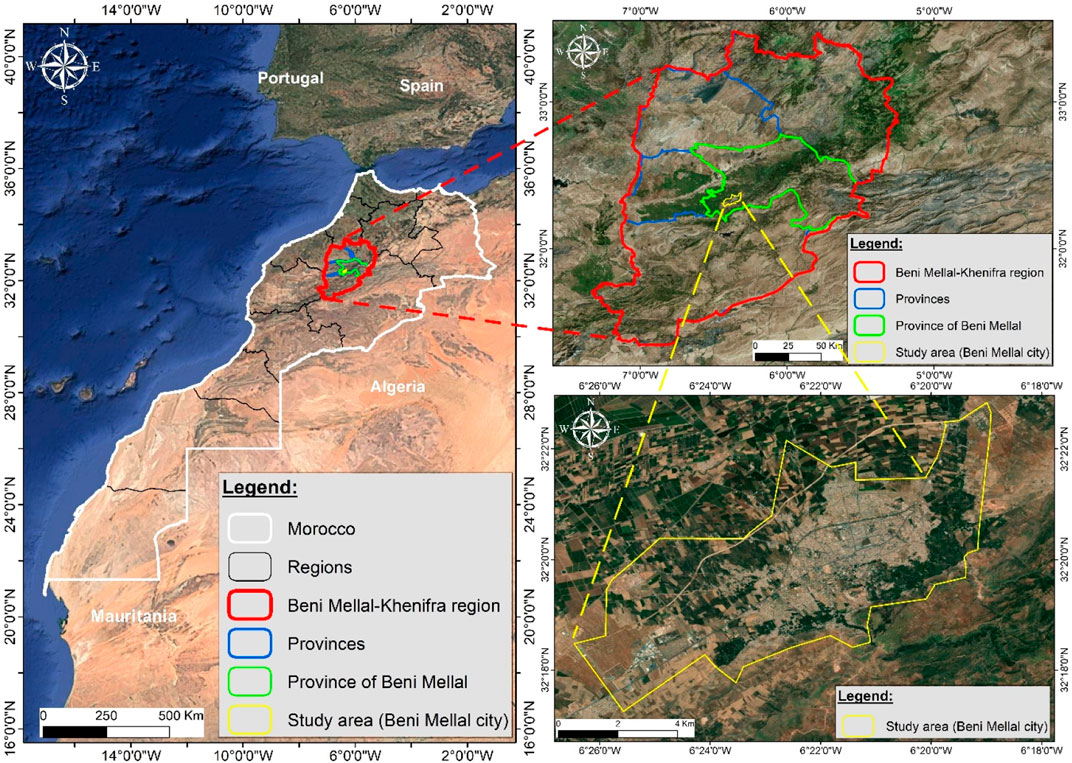
Figure 1. The geographical localization of the study area in Moroccan and regional context.

Beni Mellal serves as the capital city of the Beni Mellal-Khenifra region in Morocco. and is located at the outlet of four watersheds that seasonally trigger sudden, brief, and intense floods (Werren et al., 2016). These watersheds, from East to West, are Sabek (20.8 km2), Aïn el Ghazi (15.8 km2), Handak (29.7 km2), and Kikou (54 km2). Topographically, The Beni Mellal region is a mountainous area with altitudes ranging between 470 m and 2247 m, with the highest point called Tassemit. The climate of the area is classified as semi-arid, with continental influences, with an average temperature around 18°C. The average annual rainfall is 490 mm, with July being the driest month and March the wettest month, during which average precipitation can reach 79 mm (Barka et al., 2022).

Béni Mellal is located in the Atlas of Béni Mellal, a vast flattened anticlinal structure that rises abruptly from the plain of Béni Moussa, due to a fault system, the most important of which is the Nord-Atlas fault (Boutırame et al., 2019). The geological history of this region is linked to the formation of an intracontinental chain, resulting from geodynamic processes that took place between the end of the Paleozoic and the Mesozoic. The subsoil consists mainly of mesozoic formations based on a paleozoic base (Guezal et al., 2013). There are carbonate deposits of the middle and lower Jurassic, covered with detritic and carbonate deposits of the Cretaceous, followed by Cretaceous terrigenic deposits.

The geographical, geological, topographical and climatic characteristics of the region favour the floods. Unplanned urbanization, changes in river systems and population growth have disrupted the natural hydrological regime. This has led to an increase in flood frequency and intensity, impacting the daily lives of the inhabitants and putting pressure on sewerage and rainwater management networks.

2.2 Methodology

In this study, a comprehensive methodology (Figure 2) was adopted to assess flood hazards by integrating remote sensing, GIS, and statistical modeling. Historical flood data were compiled using Sentinel-2 and Landsat imagery, along with 12.5 m Digital Elevation Model (DEM), soil and geological maps, and road network data from OpenStreetMap (OSM). Key flood-conditioning factors including topographic, hydrological, land cover, pedologic, anthropogenic, and geological components were extracted. The dataset was split into 70% training data and 30% validation data. Three models Information Value (IV), Weighting Factor (WF), and Weight of Evidence (WoE) were applied to assess Flood hazard. Model performance was evaluated using AUC/ROC, RMSE, MAE, KAPPA, and Accuracy metrics, ensuring a reliable flood prediction system.

Figure 2

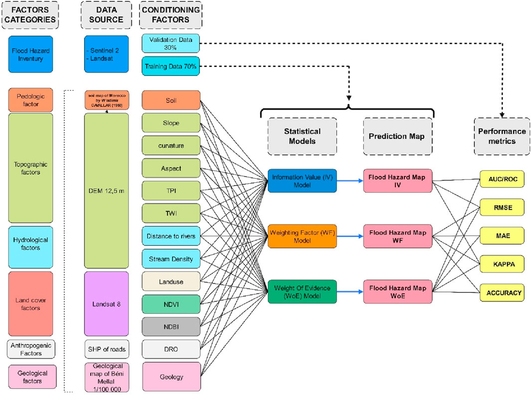
Figure 2. Flow chart of Methodology developed in this study.

The methodology of this research is outlined in the following flowchart and consists of the following steps:

⁃ Mapping the flood inventory

⁃ Identifying flood-conditioning factors

⁃ Determining the key factors for each model

⁃ Modeling and validating flood hazards

2.2.1 Urban flood inventories

We created the flood inventory for Beni Mellal using Google Earth Engine (GEE). This inventory maps flooded locations between 2000 and 2022. It served as the basis for model training and validation. We used two main satellite data collections.

First, we utilized the Landsat 7 ETM+ Collection 2 Tier 1 Surface Reflectance dataset (LANDSAT/LE07/C02/T1_L2). We filtered this collection for images between June 1, 2000, and July 1, 2010. Standard scaling factors were applied to the surface reflectance bands.

Second, we used the Sentinel-2 MSI: Multispectral Instrument, Level-2A dataset (COPERNICUS/S2_SR). This collection was filtered for images between January 1, 2019, and December 1, 2022. We applied a cloud filter, keeping only images with less than 20% cloudy pixel percentage. This common threshold improves data quality.

For both collections, we created cloud-reduced composite images. We calculated the median value for each pixel across all selected images. These median composites represent typical conditions for the respective periods. The composites were then clipped to the study area boundary.

To identify water bodies related to floods, we calculated the Normalized Difference Flood Index (NDFI). The NDFI (Equation 1) was calculated using the equation used by (Boschetti et al., 2014) determines the index values:

$\mathit{N}\mathit{D}\mathit{F}\mathit{I}=\frac{\mathit{R}\mathit{e}\mathit{d}-\mathit{R}\mathit{S}\mathit{W}\mathit{I}\mathit{R}\mathbf{2}}{\mathit{R}\mathit{e}\mathit{d}+\mathit{S}\mathit{W}\mathit{I}\mathit{R}\mathbf{2}}(1)$

For Landsat 7, we used bands SR_B3 (Red) and SR_B7 (SWIR2). For Sentinel-2, we used bands B4 (Red) and B12 (SWIR2).

We then generated a binary flood map from the NDFI composites. Pixels with NDFI values greater than or equal to 0 were classified as “Flood” (value 1). All other pixels were classified as “non-flood” (value 0). These points are in a then we converted them to raster format in a GIS environment. Therefore, we prepared a flood inventory map (Figure 3), 3112 observed points were selected from Sentinel-2 and Landsat 7. Data are typically divided into two categories: training and testing. Our literature review revealed that approximately 70% of random subsets were selected for training and calibration, with 30% for validation (Figure 4).

Figure 3

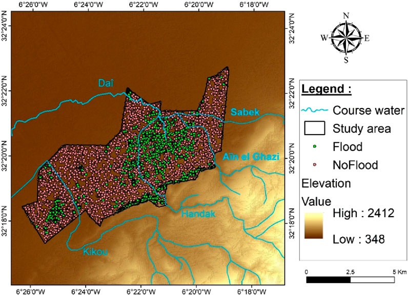
Figure 3. Inventory of training and testing data for flood prediction models.

Figure 4

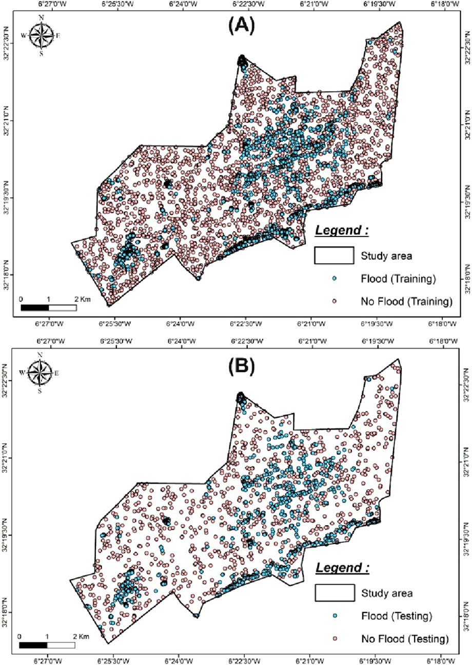
Figure 4. Flood inventory data (A) Training (70%) and (B) validation (30%) – Randomly divided.

Additionally, we conducted a field survey during heavy rainfall periods to provide ground validation. Figure 5 shows photographs from this survey, illustrating observed flooding. This fieldwork identified more than 30 specific flood locations. These independently observed field points coincided well with flood locations identified from the Sentinel-2/Landsat NDFI analysis. This congruence enhances the accuracy assessment and validates the satellite-derived inventory points.

Figure 5

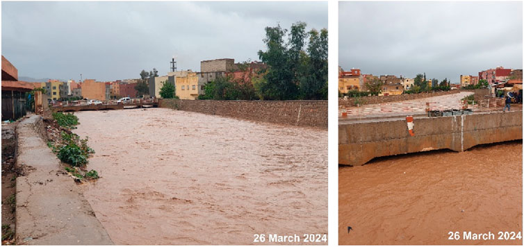
Figure 5. Ground validation photographs illustrating flooded watercourses in Beni Mellal city during the March 26, 2024 event.

2.2.2 Conditioning factors

Flood hazard assessment depends on multiple factors. These include soil (pedologic), terrain (topographic), water (hydrological), land cover, human activity (anthropogenic), and geological components. We obtained data for these factors from several sources. Key terrain data came from the ALOS PALSAR Radiometrically Terrain Corrected (RTC) High Resolution Digital Elevation Model (DEM). This product has a 12.5 m resolution and is provided by the Alaska Satellite Facility (ASF). The specific DEM used was based on data acquired July 8, 2007 (accessed on 8 August 2024). We also used Landsat 8 remote sensing data. the Geological Map of Beni Mellal (scale 1:100,000) and the Soil Map of Morocco Cavallar, W. (1950). Esquisse préliminaire de la carte des sols du Maroc au 1: 1.500. 000. Service de la Recherche Agronomique). Road network data from OpenStreetMap (OSM) provided spatial vector data.

Continuous variables required classification into intervals for the models. We used the Natural Breaks (Jenks) classification method for this purpose. This was performed using ArcGIS software. The Natural Breaks method groups similar values together effectively. It minimizes variation within classes while maximizing differences between classes. This approach is commonly applied in hazard mapping studies. Factors classified using this approach include Slope, Curvature, TWI, NDVI, NDBI, Distance to Rivers, Stream Density, and DRO. Table 1 presents the final class intervals derived for each factor.

Table 1

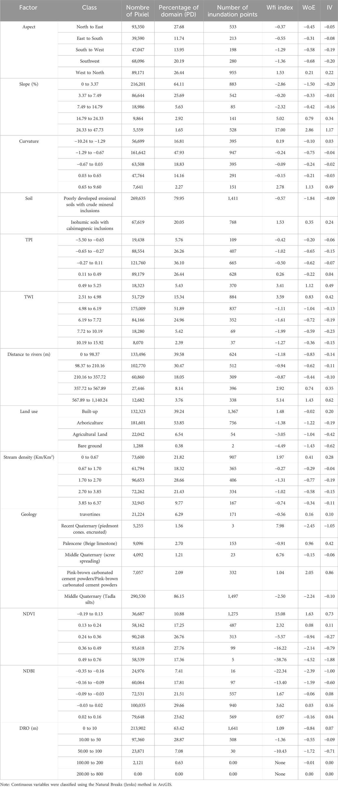
Table 1. Spatial relation between thematic layers and historic floods using FR, WOE, IV and WF Models.

2.2.2.1 Pedological and geological factors

Soil (Figure 6L) properties are fundamental in regulating infiltration and runoff, which in turn affect Flood hazard. This study utilizes pedologic factors from the Soil Map of Morocco Cavallar, W. (1950). Esquisse préliminaire de la carte des sols du Maroc au 1: 1.500. 000. Service de la Recherche Agronomique) to assess how various soil types influence water retention and permeability, shaping the area’s flood risk. The study area includes a variety of soil classifications, such as podzolic soils, podzolized red and brown soils, red soils, brown soils, and humus-carbonate soils, each with distinct hydrological properties that affect how water interacts with the landscape (Luong et al., 2021).

Figure 6

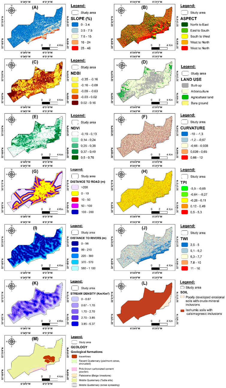
Figure 6. Flood contributing factors analyzed in this study (A) slope; (B) Aspect; (C) Normalized difference BUILT-up index (NDBI); (D) land use; (E) Normalized difference vegetation index (NDVI); (F) curvature; (G) distance to roads (DRO); (H) topographic position index (TPI); (I) distance to rivers; (J) Topographic wetness index (TWI); (K) stream density; (L) soil TYPE; (M) geology.

Similarly, geological factors were analyzed using the Geological Map of Beni Mellal (scale 1:100,000) (Barka et al., 2022), as geological formations significantly impact surface permeability and runoff behavior (Yang et al., 2020). The region consists of diverse geological structures (Figure 6M), including pink-brown carbonated cement deposits, travertines, Paleocene beige limestone, Middle Quaternary scree deposits, Recent Quaternary piedmont cones, and Middle Quaternary Tadla silts, all of which influence water flow and flood dynamics in different ways.

2.2.2.2 Topographic factors

Topographic factors strongly influence flood behavior. They control water flow, accumulation, and runoff intensity. We extracted several key parameters from the 12.5 m ALOS PALSAR RTC DEM (acquired 2007) described earlier. These parameters included:

• Slope (Figure 6A): This regulates runoff velocity. Steeper slopes accelerate water movement, increasing flood hazard (Nguyen et al., 2020).

• Curvature (Figure 6F): This affects erosion and flow patterns (Baiddah et al., 2025). Profile curvature influences flow speed changes. Plan curvature affects water convergence or divergence (Raja et al., 2017).

• Aspect (Figure 6B): This impacts sun exposure, soil moisture, and precipitation patterns. These factors indirectly affect runoff water (Peng et al., 2020).

• Topographic Position Index (TPI) (Figure 6H): TPI identifies relative elevation, aiding detection of ridges and valleys. This helps locate potential flood-prone areas (Avand et al., 2022).

• Topographic Wetness Index (TWI) (Figure 6J): TWI estimates potential soil wetness. It combines slope and upstream contributing area (Winzeler et al., 2022).

2.2.2.3 Hydrological factors

Hydrological factors are important for flood assessment. We analyzed stream density (Figure 6K) and distance to rivers (Figure 6I). We first derived the river network from the 12.5 m ALOS PALSAR RTC DEM. This involved standard GIS procedures: filling DEM sinks, calculating flow direction, and determining flow accumulation. We then applied a threshold to the flow accumulation raster to define stream channels.

Stream density was calculated from this derived network. We divided the total stream length within the basin by the basin area. Higher densities indicate greater surface runoff potential (Bogale, 2021). Distance to rivers was calculated using Euclidean distance analysis. This measured the distance from any point to the nearest DEM-extracted river channel. Proximity to rivers increases vulnerability during floods (El Bouzekraoui et al., 2024; Ibrahim et al., 2024).

2.2.2.4 Land cover factors

Land cover factors influence infiltration and runoff. We derived land use/land cover (LULC) data from Landsat 8 imagery. We performed a supervised classification to create the LULC map (Figure 6D). This involved:

• Defining Classes: Identifying key LULC types: built-up areas, agricultural land, arboriculture, and bare ground.

• Collecting Training Samples: Selecting representative pixel samples for each class directly from the Landsat 8 imagery based on visual interpretation and ground knowledge.

• Applying Algorithm: Using the Maximum Likelihood Classification algorithm in ArcGIS to assign all image pixels to one of the defined classes based on the training samples.

The resulting map shows how different covers, like impermeable built-up areas versus absorbent agricultural land, affect water behavior.

We also calculated the Normalized Difference Vegetation Index (NDVI) from the Landsat 8 imagery (Figure 6E). NDVI measures vegetation density (Ismaili et al., 2024). Higher NDVI values mean denser vegetation. Dense vegetation increases infiltration and reduces runoff, thus mitigating flood hazards (Atefi and Miura, 2022). We calculated NDVI (Equation 2) using the standard formula:

$\mathit{N}\mathit{D}\mathit{V}\mathit{I}=\frac{\mathit{N}\mathit{I}\mathit{R}-\mathit{R}}{\mathit{N}\mathit{I}\mathit{R}+\mathit{R}}(2)$

NIR is the reflectance in the Near-Infrared band (Landsat 8 Band 5). Red is the reflectance in the red band (Landsat 8 Band 4). Healthy vegetation strongly reflects NIR and absorbs Red light used for photosynthesis. Conversely, NDBI (Normalized Difference Built-Up Index) (Figure 6C), also derived from Landsat 8, highlights urban areas with impervious surfaces that intensify runoff and exacerbate flood hazards (Khan et al., 2021). NDBI (Equation 3) is computed using:

$\mathit{N}\mathit{D}\mathit{B}\mathit{I}=\frac{\mathit{S}\mathit{W}\mathit{I}\mathit{R}-\mathit{N}\mathit{I}\mathit{R}}{\mathit{S}\mathit{W}\mathit{I}\mathit{R}+\mathit{N}\mathit{I}\mathit{R}}(3)$

The Normalized Difference Built-up Index (NDBI) values range from −1 to +1. When identifying water bodies, NDBI values are negative, whereas higher values correspond to built-up areas. In contrast, vegetation exhibits low NDBI values.

2.2.2.5 Anthropogenic factors

Anthropogenic factors, particularly distance to roads (DRO), were derived from spatial vector data (SHP of roads). DRO, established using Euclidean distance analysis in GIS (Figure 6G), evaluates the impact of road networks on flood hazards. Roads increase runoff by reducing infiltration, contributing to localized flooding, particularly in urban areas (Aboutaib et al., 2023; Baiddah et al., 2023). Continuous variables required classification into intervals for the models. We used the Natural Breaks (Jenks) classification method for this purpose. This was performed using ArcGIS software. The Natural Breaks method groups similar values together effectively. It minimizes variation within classes while maximizing differences between classes. This approach is commonly applied in hazard mapping studies. Factors classified using this approach include Slope, Curvature, TWI, NDVI, NDBI, Distance to Rivers, Stream Density, and DRO. Table 1 presents the final class intervals derived for each factor.

The IG analysis revealed positive values for all 13 factors. This included TPI, Curvature, and TWI. This result indicated that each factor contributed unique predictive information. Therefore, we retained all factors for the modeling phase.

The correlation matrix (Figure 11) appears later in the Results (Section 3.5). Its primary purpose there is to visualize relationships between factors, after their individual predictive relevance was established via IG. It was not used for initial variable selection in the modeling process. The matrix also visually confirms that correlations among TPI, Curvature, and TWI were not excessively high. This provides secondary support for their inclusion.

2.2.3 Flood modeling methods

2.2.3.1 Weighting factors

The Weighting Factor (WF) method assesses flood hazard. It adapts the Statistical Index (SI) model (Oztekin and Topal, 2005; Yalcin, 2008; Khosravi et al., 2016). This approach assigns weights to conditioning factors based on their link to flood occurrences.

First, an SI value (Equation 4) is calculated for each class i within each factor. This reflects the flood density within that class compared to the study area. It uses the following formula:

$\mathit{S}\mathit{i}=\mathit{ln}\left(\frac{\frac{\mathit{N}\mathit{F}\mathit{i}}{\mathit{N}\mathit{P}\mathit{i}}}{\frac{\mathit{N}\mathit{F}\mathit{t}}{\mathit{N}\mathit{P}\mathit{t}}}\right)(4)$

where:

• NFi = number of flood pixels in class i

• NPi = total number of pixels in class i

• NFt = total number of flood pixels in the study area

• NPt = total number of pixels in the study area

Higher SI values indicate a stronger association between the factor class and flooding.

Next, these SI values are used to determine the final Weighting Factor (Wf) for each class. This involves calculating a total SI score (T (SI)) for each factor by summing the SI values weighted by the number of pixels in each class (Yalcin et al., 2011) (Equation 5):

$\mathit{T}\left(\mathit{S}\mathit{I}\right)={\displaystyle \sum _{\mathit{i}=\mathbf{1}}^{\mathit{n}}}\left(\mathit{S}\mathit{I}\right)*\mathit{S}.\mathit{p}\mathit{i}\mathit{x}(5)$

where:

SI represents the flood hazard index per factor.

S.pix represents the number of pixels in that factor class.

The Wf value is then derived by normalizing these T (SI) scores and scaling them to range from 1 to 100 (Yalcin et al., 2011) (Equation 6):

$Wf=\frac{TSI\left(value\right)-\mathit{Min}\left(TSIvalue\right)}{\mathit{Max}TSI\left(value\right)+\mathit{Min}\left(TSIvalue\right)}(6)$

where Min (T (SI)) and Max (T (SI)) are the minimum and maximum T (SI) values across all factor classes. This formula scales the results linearly to the range [1, 100].

The resulting Wf values represent the relative importance of each factor class, scaled between 1 and 100. Higher Wf values indicate a stronger influence on flood hazard. The specific calculated SI values and resulting Wf index values (scaled 1–100) for each factor class in this study are presented later (Table 1).

The Flood Hazard Map of WF Model is generated by the following (Equation 7) in ESRI ArcGIS:10.8 software:

$\mathbf{F}\mathbf{l}\mathbf{o}\mathbf{o}\mathbf{d}\mathbf{H}\mathbf{a}\mathbf{z}\mathbf{a}\mathbf{r}\mathbf{d}\left(\mathbf{\text{WF}}\right)={WF}_{Aspect}+{WF}_{Slope}+{WF}_{Curvature}+{WF}_{Soil}+{WF}_{TPI}+{WF}_{TWI}+{WF}_{Distancetorivers}+{WF}_{LandUse}+{WF}_{StreamDensity}+{WF}_{Geology}+{WF}_{NDVI}+{WF}_{NDBI}+{WF}_{DRO}(7)$

2.2.3.2 Weight of evidence

The Weight of Evidence method is frequently employed for evaluating flood hazard susceptibility (Gayen and Saha, 2017; Costache and Tien Bui, 2019). This bivariate statistical approach calculates the weights based on Bayesian probability. These weights reflect the association between each factor class and the presence or absence of flooding. The method calculates positive weights (W+) (Equation 8) and negative weights (W-) (Equation 9). These indicate the strength of evidence for flood presence or absence, respectively, given a factor class (Costache and Tien Bui, 2019), While minor variations in factor classification or handling zero counts exist in literature, this study uses the standard formulation. The calculation relies on the number of flood pixels within a class relative to the total flood pixels and the total area, as shown below:

$\mathit{W}+=\mathit{ln}\frac{\mathit{p}\left\{\mathit{B}\left|\mathit{S}\right.\right\}}{\mathit{p}\left\{\mathit{B}\left|-\mathit{S}\right.\right\}}(8)$

$\mathit{W}-=\mathbf{ln}\frac{\mathit{p}\left\{-\mathit{B}\text{−}\left|\mathit{S}\right.\right\}}{\mathit{p}\left\{\mathit{B}|-\mathit{S}\text{−}\right\}}(9)$

where P is the probability, S and -S are the presence and absence of flooding, respectively. and B and −B are the presence and absence of flood conditioning factors, respectively.

$\mathit{W}+=\frac{\frac{\mathit{N}\mathit{p}\mathit{i}\mathit{x}\mathbf{1}}{\mathit{N}\mathit{p}\mathit{i}\mathit{x}\mathbf{1}+\mathit{N}\mathit{p}\mathit{i}\mathit{x}\mathbf{2}}}{\frac{\mathit{N}\mathit{p}\mathit{i}\mathit{x}\mathbf{3}}{\mathit{N}\mathit{p}\mathit{i}\mathit{x}\mathbf{3}+\mathit{N}\mathit{p}\mathit{i}\mathit{x}\mathbf{1}}}(10)$

$\mathit{W}-=\frac{\frac{\mathit{N}\mathit{p}\mathit{i}\mathit{x}\mathbf{2}}{\mathit{N}\mathit{p}\mathit{i}\mathit{x}\mathbf{1}+\mathit{N}\mathit{p}\mathit{i}\mathit{x}\mathbf{2}}}{\frac{\mathit{N}\mathit{p}\mathit{i}\mathit{x}\mathbf{4}}{\mathit{N}\mathit{p}\mathit{i}\mathit{x}\mathbf{3}+\mathit{N}\mathit{p}\mathit{i}\mathit{x}\mathbf{1}}}(11)$

In the study by Costache and Tien Bui (2019) the Weight of Evidence (WOE) coefficient is calculated using a specific formula that quantifies the predictive influence of different spatial data layers based on their association with flood events. The Weight of Evidence approach is a bivariate statistical method commonly used in spatial analysis, particularly in environmental and geological assessments.

The WOE coefficient for each factor is calculated using Equation 12 below:

$\mathbf{\text{WOE}}=\left(\mathit{W}+\right)-\left(\mathit{W}-\right)(12)$

The Flood Hazard Map of WOE Model is generated by the following Equation 12 in ESRI ArcGIS:10.8 software:

$\mathbf{F}\mathbf{l}\mathbf{o}\mathbf{o}\mathbf{d}\mathbf{H}\mathbf{a}\mathbf{z}\mathbf{a}\mathbf{r}\mathbf{d}\left(\mathbf{\text{WOE}}\right)={\text{WOE}}_{Aspect}+{\text{WOE}}_{Slope}+{\text{WOE}}_{Curvature}+{\text{WOE}}_{Soil}+{\text{WOE}}_{TPI}+{\text{WOE}}_{TWI}+{\text{WOE}}_{Distancetorivers}+{\text{WOE}}_{LandUse}+{\text{WOE}}_{StreamDensity}+{\text{WOE}}_{Geology}+{\text{WOE}}_{NDVI}+{\text{WOE}}_{NDBI}+{\text{WOE}}_{DRO}(13)$

2.2.3.3 Information value (IV)

The Information Value Model (IV) is another statistical approach often used for the analysis of Flood hazard (Addis, 2023; Rojas et al., 2023). It calculates an index reflecting the influence of different factor classes on flood occurrence. The IV method uses statistical indices to assess the predictive power of each class based on the proportion of floods occurring within it.

The Information Value (IV) for a class i of a specific factor is calculated as follows (Equation 14):

$\mathit{I}\mathit{V}=\mathbf{log}\left(\left(\frac{{\mathit{D}}_{\mathit{i}}}{{\mathit{N}}_{\mathit{i}}}\right)/\left(\frac{{\mathit{D}}_{\mathit{t}}}{{\mathit{N}}_{\mathit{t}}}\right)\right)(14)$

where:

D_i: Number of pixels (or points) of floods in class i.

N_i: Total number of pixels (or points) in class ii.

D_t: Total number of pixels (or points) of floods throughout the study area.

N_t: Total number of pixels (or points) throughout the study area.

The higher the IV, the more the class contributes to the occurrence of floods.

Flood Hazard Map of IV Model is generated by the following Equation 15 in ESRI ArcGIS:10.8 software:

$\mathbf{F}\mathbf{l}\mathbf{o}\mathbf{o}\mathbf{d}\mathbf{H}\mathbf{a}\mathbf{z}\mathbf{a}\mathbf{r}\mathbf{d}\left(\mathit{I}\mathit{V}\right)={IV}_{Aspect}+{IV}_{Slope}+{IV}_{Curvature}+{IV}_{Soil}+{IV}_{TPI}+{IV}_{TWI}+{IV}_{Distancetorivers}+{IV}_{LandUse}+{IV}_{StreamDensity}+{IV}_{Geology}+{IV}_{NDVI}+{IV}_{NDBI}+{IV}_{DRO}(15)$

2.2.4 Calculation of information gain (IG)

In the context of flood prediction, Information Gain (IG) is a key metric used to assess the influence of environmental factors on flood occurrence. It quantifies the reduction in uncertainty (entropy) about flood events when data is split based on a specific environmental variable.

Information Gain (IG) was used to measure the importance of 13 environmental factors influencing floods.

The IG (Equation 16) for a given environmental factor X is then computed as:

$\mathbf{\text{IG}}\left(\mathbf{S},\mathbf{X}\right)=\mathbf{H}\left(\mathbf{S}\right)-\mathbf{H}\left(\mathbf{S}|\mathbf{X}\right)(16)$

where:

H(S) is the initial entropy (Equation 17) before splitting the data.

The IG method is based on Shannon’s entropy theory, where entropy measures the degree of randomness in a dataset. The formula for entropy is:

$\mathbf{H}\left(\mathbf{S}\right)=-{\displaystyle \sum _{\mathit{n}=\mathbf{1}}^{\mathit{n}}}\mathit{P}\left({\mathit{C}}_{\mathit{i}}\right)\mathbf{log}\mathbf{2}\mathit{P}\left({\mathit{C}}_{\mathit{i}}\right)(17)$

where:

S represents the dataset containing flood and non-flood locations.

Ci denotes the class labels (flooded or non-flooded).

P(Ci) is the probability of each class in the dataset.

n is the number of classes.

H(S|X) is the conditional entropy (Equation 18), calculated as:

$\mathbf{H}\left(\mathbf{S}|\mathbf{X}\right)={\displaystyle \sum _{\mathit{v}\in \mathit{V}\mathit{a}\mathit{l}\mathit{u}\mathit{e}\mathit{s}\left(\mathit{X}\right)}}\mathit{P}\left(\mathit{v}\right)\mathit{H}\left({\mathit{S}}_{\mathit{v}}\right)(18)$

where:

P($\mathit{v}$) represents the proportion of data in each category of factor X.

H(S_v) is the entropy within each category after partitioning.

A higher IG value indicates that the factor significantly reduces uncertainty, meaning it has a stronger influence on flood prediction.

2.2.5 Prediction performance methods

In this study, we used RStudio to evaluate how well the prediction models performed. By using different metrics like AUC/ROC, Cohen’s Kappa, RMSE, MAE, and accuracy, we were able to get a clear picture of each model’s strengths and weaknesses. This comprehensive approach helped us compare the models and better understand their overall reliability and effectiveness.

2.2.5.1 AUC/ROC

Before building the models, the predictive performance of various methods was assessed using the receiver operator characteristic-area under the curve (ROC-AUC) metric based on test data (Ismaili et al., 2023). The ROC curve is a fundamental tool in spatial modeling, which effectively visualizes the trade-off between specificity and sensitivity. Here’s a breakdown of the key elements involved:

Specificity: This is plotted on the x-axis and refers to the ability of the model to correctly identify non-flood locations as such. It is calculated as the proportion of true negative results (TN) among all non-flood observations.

Sensitivity: Also known as recall or true positive rate, this is plotted on the y-axis and measures the proportion of actual flood locations that are accurately predicted. It represents the model’s ability to detect all relevant instances.

The Area Under the Curve (AUC) is a crucial metric that quantifies the overall ability of the ROC curve to distinguish between the classes—flood and non-flood in this context. An AUC value ranges from 0 to 1, where:

0 represents a model with no discriminative ability, 0.5 suggests a performance no better than random chance,

1 indicates perfect classification.

The AUC is calculated using Equation 19 below:

$\mathit{A}\mathit{U}\mathit{C}=\frac{\left(\mathit{\Sigma }\mathit{T}\mathit{P}+\mathit{\Sigma }\mathit{T}\mathit{N}\right)}{\mathit{P}+\mathit{N}}(19)$

where:

ΣTP (Sum of True Positives): The total number of flood locations correctly identified as flood.

ΣTN (Sum of True Negatives): The total number of non-flood locations correctly identified as non-flood.

P (Positives): The total number of actual flood locations (pixels with torrential phenomena).

N (Negatives): The total number of actual non-flood locations (pixels without torrential phenomena).

This formula essentially captures the proportion of true results (both true positives and true negatives) among the total cases examined, providing a measure of the model’s accuracy in classifying each pixel correctly. This comprehensive evaluation helps in determining the most effective models to include in an ensemble for improved predictive performance.

2.2.5.2 MAE (Mean Absolute Error)

Mean Absolute Error (MAE) is valuable when predicting quantitative aspects of flooding, such as water levels or flow rates at specific gauge stations. It gives an average of the absolute errors between predicted values and observed values, providing a clear measure of prediction error in the same units as the prediction itself (Haghizadeh et al., 2017; Janizadeh et al., 2021).

The MAE (Equation 20) is calculated using the equation below:

$\mathit{M}\mathit{A}\mathit{E}=\frac{\mathbf{1}}{\mathit{n}}{\displaystyle {\sum }_{\mathit{i}=\mathbf{1}}^{\mathit{n}}}\left|{\mathit{y}}_{\mathit{i}}-{\widehat{\mathit{y}}}_{\mathit{i}}\right|(20)$

where:

n is the number of observations.

${\mathit{y}}_{\mathit{i}}$ is the actual (observed) value for the i-th observation.

${\widehat{\mathit{y}}}_{\mathit{i}}$ Is the predicted value for the i-th observation.

$\mid {\mathit{y}}_{\mathit{i}}-{\widehat{\mathit{y}}}_{\mathit{i}}\mid$ is the absolute difference between the actual and predicted values.

2.2.5.3 RMSE (Root Mean Square Error)

Root Mean Square Error (RMSE) is particularly effective for quantitative forecasts, such as predicting water levels or flow rates. Its value lies in the way it disproportionately penalizes larger errors over smaller ones. This attribute is critical in flood prediction, where underestimating the impact of an event can have more severe consequences than overestimating it (Haghizadeh et al., 2017; Janizadeh et al., 2021).

These metrics can help determine how reliable and accurate a flood prediction model is in practical scenarios. Moreover, they can guide improvements in model development and deployment, ensuring better preparedness and response strategies for flood-prone areas (Haghizadeh et al., 2017; Janizadeh et al., 2021).

The RMSE (Equation 21) is calculated using the equation below:

$\mathit{R}\mathit{M}\mathit{S}\mathit{E}=\sqrt{\frac{\mathbf{1}}{\mathit{n}}{\sum }_{\mathit{i}=\mathbf{1}}^{\mathit{n}}{\left({\mathit{y}}_{\mathit{i}}-{\widehat{\mathit{y}}}_{\mathit{i}}\right)}^{\mathbf{2}}}(21)$

where:

n is the number of observations.

${\mathit{y}}_{\mathit{i}}$ is the actual (observed) value for the i-th observation.

${\widehat{\mathit{y}}}_{\mathit{i}}$ Is the predicted value for the i-th observation.

${\left({\mathit{y}}_{\mathit{i}}-{\widehat{\mathit{y}}}_{\mathit{i}}\right)}^{\mathbf{2}}$ is the squared difference between the actual and predicted values.

2.2.5.4 Kappa

Cohen’s Kappa is a statistical tool. It measures agreement between two sets of predictions (e.g., model output vs. reality), (Equation 22) It accounts for agreement occuring by chance alone (Feuerman and Miller, 2008). Kappa is useful for evaluating prediction models. This is especially true for models producing categories, like flood versus non-flood areas Cohen’s Kappa can be used to assess the performance of different models and measure inter-rater reliability.

The equation for Kappa (Cohen’s Kappa) is:

$\mathit{k}=\frac{{\mathit{p}}_{\mathbf{0}}-{\mathit{p}}_{\mathit{e}}}{\mathbf{1}-{\mathit{p}}_{\mathit{e}}}(22)$

where:

${\mathit{p}}_{\mathbf{0}}$ is the observed agreement, which is the proportion of times the two raters (or the model and ground truth) agree.

${\mathit{p}}_{\mathit{e}}$ is the expected agreement, which is the proportion of times the two raters (or model and ground truth) would agree by chance.

2.2.5.5 Accuracy

Accuracy is a straightforward measure (Equation 23) when predicting whether a flood will occur or not (binary classification: flood/no flood). It provides a quick snapshot of overall model effectiveness (El Haou et al., 2025) but can be misleading if the data set is unbalanced (e.g., very few flood events compared to non-flood days).

The equation for Accuracy is:

$\mathit{A}\mathit{c}\mathit{c}\mathit{u}\mathit{r}\mathit{a}\mathit{c}\mathit{y}=\frac{\mathbf{T}\mathbf{P}+\mathbf{T}\mathbf{N}}{\mathbf{T}\mathbf{P}+\mathbf{T}\mathbf{N}+\mathbf{F}\mathbf{P}+\mathbf{F}\mathbf{N}}(23)$

where:

TP (True Positives): The number of correctly predicted flood events.

TN (True Negatives): The number of correctly predicted non-flood events.

FP (False Positives): The number of non-flood events incorrectly predicted as floods.

FN (False Negatives): The number of flood events incorrectly predicted as non-floods.

3 Results

3.1 Classification of classes influencing flood hazards according to prediction models

The analysis of flood hazard involves various factors that contribute to the overall risk. Table 1 provides a comprehensive breakdown of these factors, categorized by classes such as Aspect, Slope, Curvature, Soil, TPI, TWI, Distance to Rivers, Land Use, Stream Density, Geology, NDVI, NDBI, and DRO. Each class is analyzed based on the Weighting Factor (WF), Weight of Evidence (WOE), and Information Value (IV) index. These indices help to normalize the data and provide a clear picture of the relative importance of each class in predicting flood hazards (El Haou et al., 2025). In the following sections, we will classify and discuss these classes according to the three different prediction models used in this study.

3.2 Classification of key factors in the information value (IV) model

The analysis of the information value (IV) highlights the main factors influencing flood Hazard (Figure 7). The dominant factor is the slope (24.33%–47.73%) with the highest information value, confirming its essential role in runoff and flood dynamics. The steeper the slopes, the faster the runoff, reducing infiltration and increasing the concentration of downstream flows. The second most influential factor is the curvature (0.65–9.60), which represents the characteristics of the shape of the terrain and its influence on the accumulation or disposal of water. Higher curvature indicates convex areas promoting flow, while negative curvatures are associated with water-retaining depressions. The aspects of the field also play an important role, in particular the West-North orientation, which appears to be a key direction influencing flood Hazard. Other slope classes, including (14.79 per cent to 24.33 per cent) and (7.49 per cent to 14.79 per cent), as well as specific terrain orientations (South-West, East-South, North-East) are also identified as having a moderate to low impact on floods. Finally, specific classes of curvature (−1.29 to 0.67), (−10,24 to −1.29), (0.03–0.65), (−0.67 to 0.03) and slope (3.37%–7.49%) have lower information values, indicating a secondary role in the determination of flood Hazard.

Figure 7

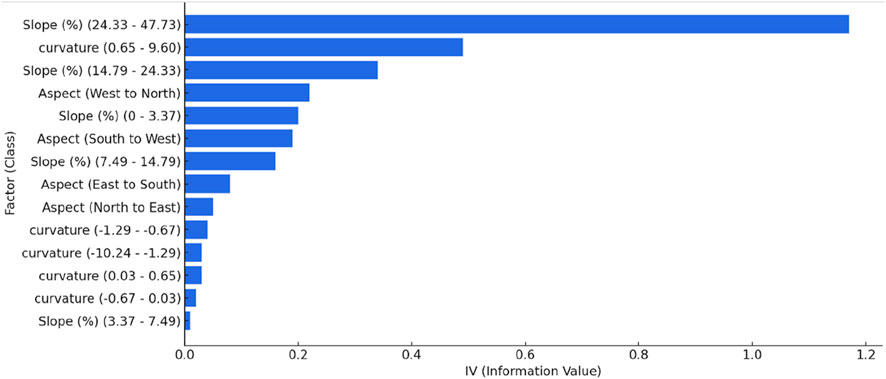
Figure 7. Top 15 factors (classes) influencing flood hazard based on information value (IV) Model.

3.3 Classification of key factors in weight factor (WF) model

The analysis of the WF Model highlights the main factors influencing the risks of flooding in the study area (Figure 8). The most important factor is the slope (24.33 per cent to 47.73 per cent), stressing that steep slopes promote increased susceptibility to flooding. This correlation indicates that the inclined terrain facilitates the rapid flow of runoff, thereby reducing infiltration and increasing downstream water accumulation. In second place, the NDVI (−0.19 to 0.13) plays a key role in flood regulation, highlighting the importance of vegetation cover. A higher plant density promotes infiltration, limits runoff and thus contributes to the reduction of the risk of flooding.

Figure 8

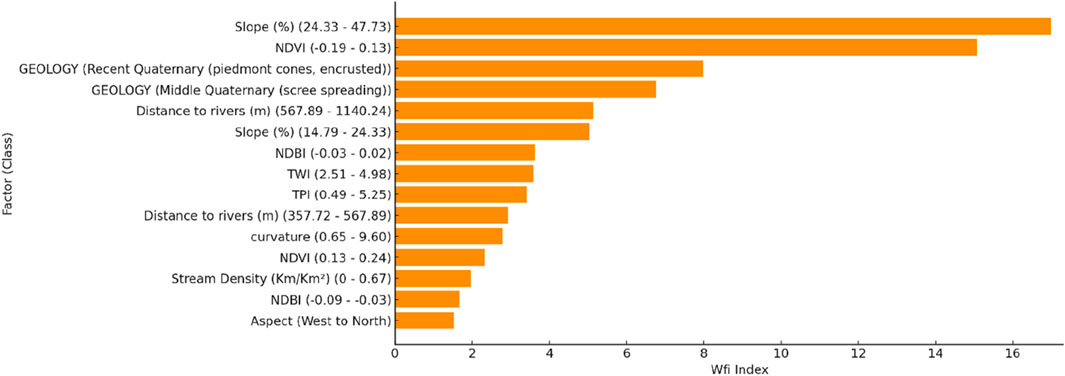
Figure 8. Top 15 factors (classes) influencing flood hazard based on weight factor (WF) Model.

Geological factors also occupy a preponderant place, with Recent Quaternary deposits (piedmont cones, encrusted) and Middle Quaternary deposits (scree spreading), which influence the permeability of the soil and modulate the behavior of the flows. In addition, the proximity of rivers (567.88–1,140.24 m) is proving to be a key factor, with areas near rivers being more exposed to floods due to potential overflows and lateral water expansion.

Other influential parameters include NDBI (0.03–0.08), TWI (1.51–4.98) and IPT (0.9–5.85), which reflect the hydrological and geomorphological characteristics of floods. The curvature (0.165–0.960), the stream densnity (km/km2: 0–0.67) and the orientation of the terrain (West to North) provide further details to the flood risk assessment model.

3.4 Classification of key factors in weight of evidence (WOE) model

The analysis of the Weight of Evidence (WoE) highlights the main factors influencing Flood hazard in the study area (Figure 9). The slope (24.33%–47.73%) is the dominant factor, highlighting its key role in the dynamics of runoff and infiltration. The steeper terrain accelerates the runoff of rainwater, increasing the risk of flooding downstream.

Figure 9

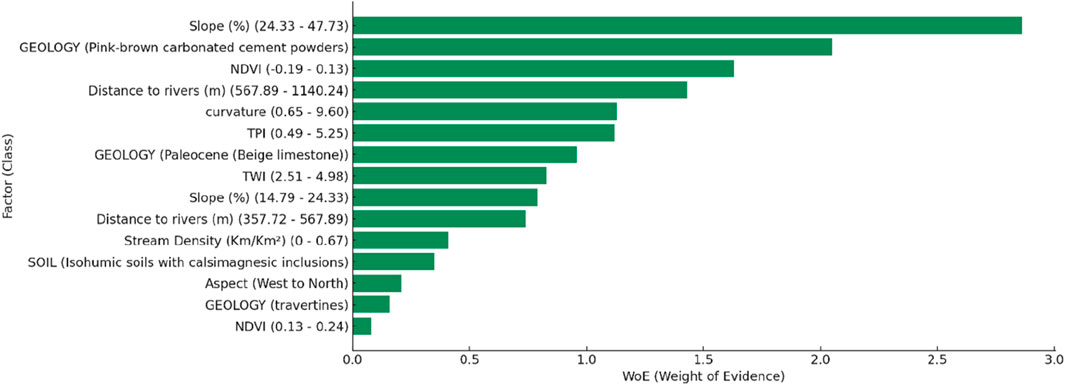
Figure 9. Top 15 factors (classes) influencing flood hazard based on weight of evidence (WOE) Model.

Geological factors also play a important role, including the presence of formations such as pink-brown carbonate powders and beige Paleocene limestones. These structures influence soil permeability and water infiltration capacity, thereby altering accumulation and flow conditions.

NDVI (−0.19 to 0.13) is another key factor, highlighting the role of vegetation cover in flood regulation. Dense vegetation improves infiltration and reduces surface run-off, while stripped areas are more vulnerable to rapid run-off.

Hydrological factors are also predominant, with distance to rivers (567.89–1,140.24 m) indicating that areas close to rivers have a higher probability of flooding. In addition, parameters such as curvature (0.65–9.60), IPT (0.9–5.25) and TWI (1.51–4.98) confirm the influence of terrain morphology on water accumulation and distribution.

Secondary factors, such as the density of the hydrographic network (0–0.67 km/Km2), the orientation of the terrain (West to North), and certain soil types (isohumous soil with callimagnesic inclusions), complete the analysis model. Finally, the presence of travertines and NDVI classes (0.13–0.24) shows a minor but nevertheless significant effect on the dynamics of floods.

3.5 Information gain analysis of flood conditioning factors

The analysis utilizing the Information Gain for the IV, WF, and WoE approaches is shown in (Figure 10) reveals the differing significance of environmental variables in Flood hazard mapping. The NDVI (Normalized Difference Vegetation Index) showed the highest IG for all three approaches, with an especially high weighting in the WF approach (77.95), indicating the importance of vegetation cover in controlling surface runoff and infiltration. Slope also showed a high impact on Flood hazard, with IG values of 27.4 (WF) and 4.44 (WoE), attesting to the effect of topography on water flow patterns. Other significant factors include geology, river proximity, and NDBI (Normalized Difference Built-up Index), which together attest to the multifaceted interaction between natural and anthropogenic factors in controlling flood-prone zones. The WF approach consistently allocated higher IG values, indicating a high differentiation between flood-prone and non-flood-prone zones, while the WoE approach yielded more even weighting across variables. All 13 factors demonstrated positive Information Gain and were included in the analysis (Tehrany et al., 2019).

Figure 10

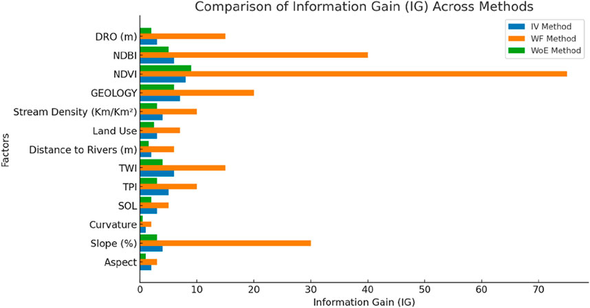
Figure 10. Comparison of information gain (IG) across models.

To identify which variables are significantly related to each other and to understand the interplay between different factors in assessing flood hazards we used a correlation matrix (Figure 11) that visualizes the relationships between various factors influencing flood hazards (Mahdizadeh Gharakhanlou and Perez, 2023). Each cell in the matrix represents the correlation coefficient (ranging from −1 to 1) between two variables, indicating the strength and direction of their relationship.

Figure 11

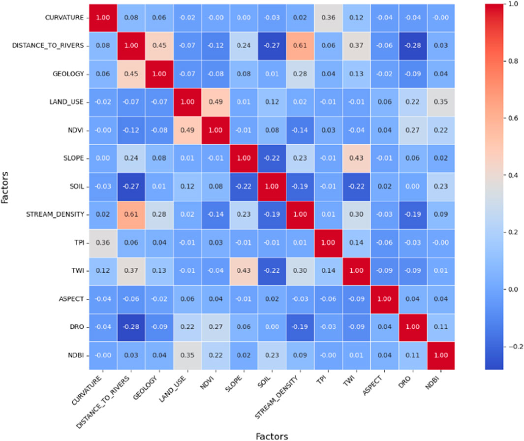
Figure 11. Correlation matrix of the flood influencing factors considered in the present study.

Factors such as NDBI, DRO, and TWI appear to have several positive correlations with other variables, indicated by the darker red boxes. For example, TWI has a strong correlation with DRO. Other pairs of factors, such as CURVATURE and DISTANCE TO RIVERS, appear to have little or no significant correlation, as indicated by the lighter boxes.

3.6 Models’ predictive capability

3.6.1 ROC curves analyze performances

The Comparison between training and test data (Figure 12) ROC curves analyze performances of the three methods utilized in flood modelling: Weight of Frequency (WF), Information Value (IV), and Weight of Evidence (WOE).

Figure 12

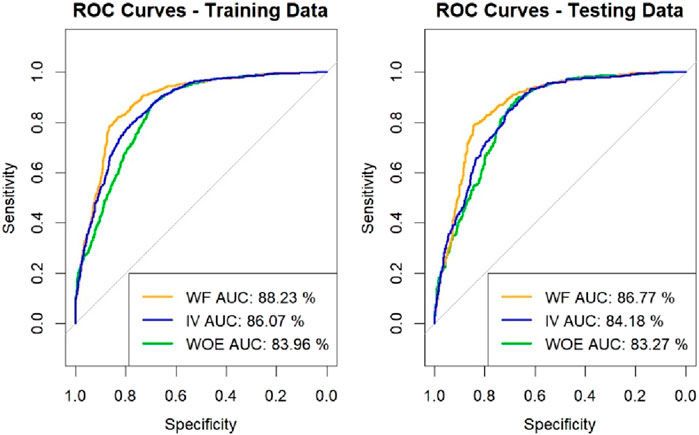
Figure 12. ROC Curves for Training and Testing Data using WF, IV, and WOE Models.

For training data, the area under the curve (AUC) is the highest for the WF method (88.23%), followed by IV (86.07%) and WOE (83.96%). This indicates that the WF method has the best predictive capacity on the learning set.

For test data, the trend is similar with an AUC of 86.77% for WF, 84.18% for IV, and 83.27% for WOE. Although performance is slightly reduced on the test set, the WF method remains the most effective in predicting Flood hazard.

Analysis of the ROC curves shows that all methods offer good discrimination between the prone and non-flooded areas. However, the WF method demonstrates better stability and higher accuracy both on the training package and on the test set.

3.6.2 Performances metrics

In The comparative evaluation of the Weight of Evidence (WoE), Weight of Frequency (WF) and Information Value (IV) models was performed using several performance metrics: Accuracy, Kappa, RMSE and MAE (Figure 13).

Figure 13

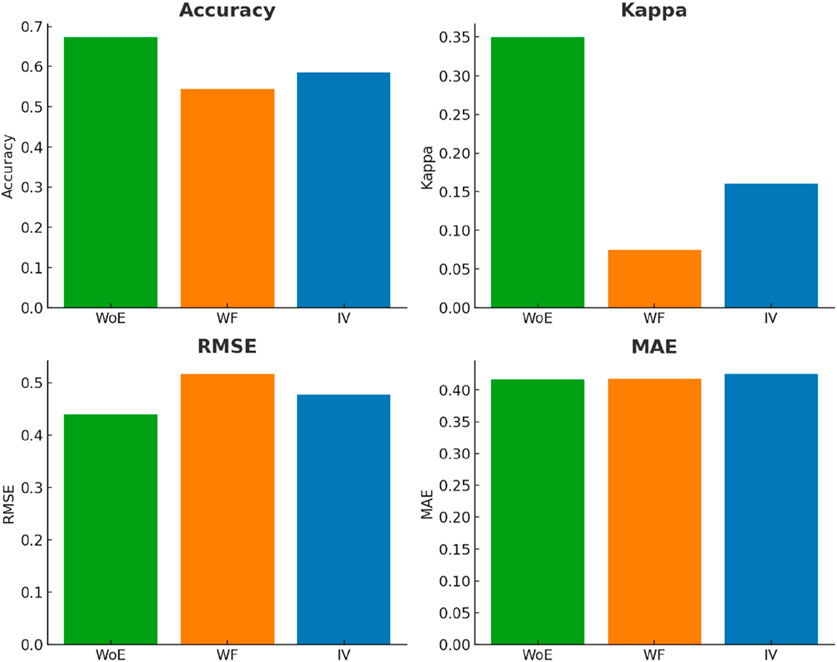
Figure 13. Bar chart comparing three predictive models using multiple performance metrics: Accuracy, Mean Absolute Error (MAE) and Root Mean Square Error (RMSE).

Accuracy: The WoE method achieves the best accuracy, followed by IV and WF. This indicates that WoE performs better at properly classifying flood-prone areas.

Kappa: The Kappa Index, which measures the agreement between prediction and reality by taking into account randomness, is the highest for WoE, followed by IV and WF. This confirms that WoE has greater consistency in its predictions.

RMSE (Root Mean Square Error): The WF method has the highest mean square error, indicating a greater dispersion of prediction errors. WoE displays the best performance with the lowest RMSE, followed by IV.

MAE (Mean Absolute Error): the results are similar for all models, suggesting that the mean amplitude of prediction errors is similar to each other, however with slight WoE superiority.

3.7 Urban flood hazard probability mapping

3.7.1 Flood hazard map using IV method

The map of flood hazard using IV model (Figure 14) show that 28.5% of the territory is classified as high or very high, with a high concentration in the south and south-east areas, where topographical conditions increase vulnerability to floods. Moderate areas (24.5%) are located in transition regions between steep slopes and plains, while low- and very low-risk areas (47%) occupy the North and West sectors, where conditions favour better water infiltration.

Figure 14

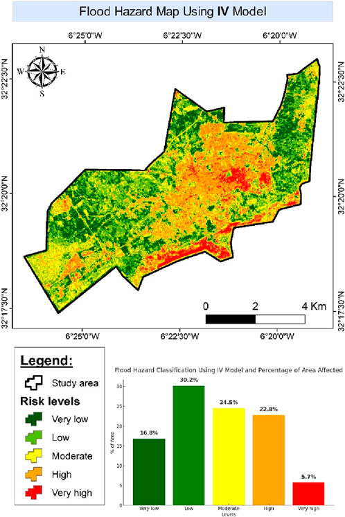
Figure 14. Flood hazard map generated IV method.

High-risk areas are dominated by steep slopes (more than 24%), an unfavorable terrain and strong curvature, which intensifies runoff and reduces infiltration. Proximity to rivers is also a key factor, with more than 50% of floods recorded within 600 m of rivers. The effects of terrain morphology (high TWI, high curvature and specific slope exposure) reinforce these phenomena by creating conditions conducive to the accumulation of rainwater.

3.7.2 Flood hazard map using WF model

Flood hazard map generated by WF Model (Figure 15) reveal a concentration of high and very high-risk areas (44.7%) mainly in the south and south-east of the study area. This trend is strongly linked to the slope, where 45% of high-risk areas are located on high-density terrain, promoting rapid runoff and limiting infiltration. Moreover, the recent and middle Quaternary geological formations, covering almost 50% of flood-prone areas, have a low permeability which accentuates the accumulation of surface water.

Figure 15

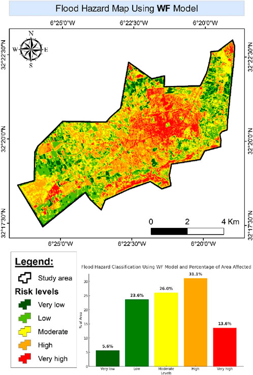
Figure 15. Flood hazard map generated WF method.

Urbanization also plays a key role, with 26% of moderately to heavily flood-prone areas in high NDBI-index sectors. Waterproofing of soils reduces infiltration and promotes run-off. In addition, the presence of travertines in the city center influences the dynamics of water, making some areas more vulnerable. The topographical humidity index (TWI) shows areas of stagnation, corresponding to 31% of high-risk areas, especially in natural depressions and alluvial plains. Finally, proximity to watercourses remains a critical factor, with more than 50% of flood-prone areas less than 600 m from rivers, exposing these areas to floods and overflows.

3.7.3 Flood hazard map using WoE method

The map of WoE model (Figure 16) shows that 18.2% of the territory is classified as high or very high, mainly located in the South and Southeast, where topographical and geological conditions increase vulnerability to floods. Moderately exposed areas (31.2%) are distributed in the transition zones between reliefs and plains, while 50.6% of the territory is low to very low, especially in the West and North, where infiltration conditions are more favorable.

Figure 16

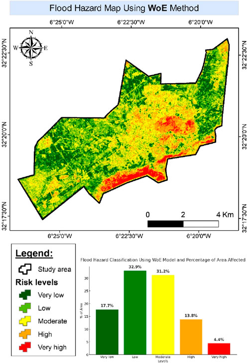
Figure 16. Flood hazard map generated WOE method.

The most sensitive areas are characterized by a high slope (more than 24%), a proximity to rivers (50% of floods less than 600 m from a river) and poorly permeable geological formations (cemented carbonate-based powders and formations of the recent and medium Quaternary). Urbanization also plays a key role, with 26% of flood-prone areas in NDBI-indexed areas, where soil sealing accentuates runoff. The topographical humidity index (TWI) shows areas of stagnation in alluvial depressions and plains, coinciding with 31.2% of areas classified at moderate to high risk.

4 Discussion

4.1 Influence of key factors on flood hazard

Our results with the WF, WoE and IV models confirm that several factors play a key role in Flood hazard, in agreement with studies by Suppawimut (2021), Mousavi et al. (2022), Islam (2024). The impact of slope is particularly significant: areas with steep slopes promote rapid runoff, limiting infiltration and increasing the risk of flooding downstream. This observation is shared by Suppawimut (2021), Islam (2024), who emphasize the importance of topography in the distribution of water flows. Further supporting slope’s relevance, studies using multi-criteria decision-making (MCDM) approaches, such as Goumghar et al. (2025) in Morocco and Hossain and Mumu (2024) in Bangladesh, identified slope as a critical factor. This confirms its importance across different modeling methods and regions. However, our results show that low-slope areas are also vulnerable, in particular due to the prolonged accumulation of surface water, a trend also identified by Mousavi et al. (2022) with the WoE model.

Another key factor is proximity to rivers, which strongly influences the spatial distribution of floods. Our results indicate that more than 50% of floods occur within 600 m of rivers, confirming the observations of (Mousavi et al., 2022; Islam, 2024). This consistency extends to studies using MCDM approaches ((Hossain and Mumu, 2024; Goumghar et al., 2025) and statistical methods like FR and SE (Chetia and Paul, 2024). These methods generally rank river proximity or related metrics highly. Riparian area vulnerability is increased by rapid soil saturation and inadequate channel capacity during extreme rainfall. This highlights the need to integrate hydrodynamic models into risk assessment.

On the other hand, a notable divergence with previous studies lies in the importance given to vegetation cover (NDVI) (El Haou et al., 2025). While (Suppawimut, 2021) puts more emphasis on land use, our results demonstrate that vegetation plays a key role in soil stabilization and precipitation absorption, thus helping to reduce surface runoff. This finding is supported by (Hossain and Mumu, 2024), who included NDVI in their MCDM assessment, and (Chetia and Paul, 2024), who linked specific NDVI ranges to flood susceptibility. Studies like (Mentzafou et al., 2017) also highlight specific land use vulnerabilities (e.g., agricultural areas), aligning with the idea that land cover influences flood dynamics. Accounting for both ecological (NDVI) and anthropogenic (land use, identified by (Chetia and Paul, 2024; Hossain and Mumu, 2024; Goumghar et al., 2025) factors could refine model accuracy. Another factor that is often underestimated is soil moisture, assessed via the Topographic Moisture Index (TWI) in the WoE model. Our results show that 31% of floods occur in areas with high TWI, confirming that soil moisture plays a major role in precipitation retention and runoff. This observation is consistent with the findings of Marchandise and Viel (2009), who noted that soil moisture strongly influences seasonal variations in flooding. Including TWI as a key factor (Chetia and Paul, 2024; Hossain and Mumu, 2024) reinforces its importance. Integrating TWI improves identification of water stagnation areas and flood prediction when soils are saturated. Finally, the analysis of the curvature of the ground reveals that convex zones facilitate the rapid evacuation of water, while concave zones act as natural retention basins, thus modifying local flood dynamics. The interplay between topography (elevation, slope, curvature, TWI, flow accumulation) (Goumghar et al., 2025), hydrology (river proximity, drainage density) (Chetia and Paul, 2024; Hossain and Mumu, 2024), geology (Mentzafou et al., 2017), land cover/vegetation, and rainfall (common factors in most studies) confirms risk mapping requires multiple factors. Increasing urbanization and the effects of climate change, it is more important than ever to take these dynamics into account in order to better manage risks and adapt infrastructure to local hydrological realities.

4.2 Comparison of models based on performance

Evaluation of the performance of our models shows that WoE and IV offer more stable and accurate results than WF. Our analyses indicate that the AUC of the Model IV reaches 86.07% in training and 84.18% in testing, while WoE shows 83.96% and 83.27%, respectively. These values are comparable to those obtained by Mousavi et al. (2022), Islam (2024), reinforcing the validity of the models in different geographical areas. Interestingly, our statistical models’ performance metrics are comparable to those reported for MCDM models in similar contexts. For instance, Goumghar et al. (2025) reported an AUC of 0.882 using their multi-criteria model in Morocco, while Hossain and Mumu (2024) achieved 0.848 using their approach in Bangladesh. This suggests well-calibrated statistical models can match expert-driven MCDM approaches in predictive performance for flood susceptibility. On the other hand, although the WF model has high AUCs (88.23% in training and 86.77% in testing), they are still lower than those obtained by Suppawimut (2021) (93.06% for WF), suggesting potential improvement by integrating real-time hydrodynamic or climate data (Chetia and Paul, 2024). found lower AUCs for FR (0.748) and SE (0.761) models in Assam, possibly due to data differences or regional complexity (Mentzafou et al., 2017). using a GIS-based multi-criteria model, reported satisfactory performance, indicating the general utility of integrating multiple factors.

Analysis of error metrics confirms. WoE’s robustness, showing the lowest RMSE and MAE values, indicating better robustness and an ability to reduce extreme errors. The Kappa index is also higher for WoE, reflecting better consistency in the classification of flood zones. Conversely, WF shows the lowest scores in terms of accuracy and Kappa agreement, suggesting increased sensitivity to imbalances in the data.

4.3 Improved models and perspectives

Although our models capture major flooding types, limitations exist, especially in urban areas. The WoE model analysis (26% of floods in urban zones) indicates ignoring drainage infrastructure may overestimate risk. Stormwater systems significantly alter flood dynamics compared to natural areas. Integrating data on urban water infrastructure is needed for more precise urban flood assessment.

Furthermore, this study evaluated only three statistical techniques. A direct comparison with machine learning algorithms (Random Forest, SVM, Neural Networks) was not performed. ML models might better capture complex factor interactions and could improve predictive accuracy. Future research comparing statistical and ML methods in Béni Mellal is recommended to identify optimal modeling strategies.

Another key limitation is the focus on hazard susceptibility. Comprehensive risk assessment requires integrating our hazard maps with socio-economic vulnerability data (population density, building types, poverty, etc.). This would quantify potential damages (costs, displacement) and identify the most vulnerable communities, following approaches similar to Hossain and Paul (2018). Future work should prioritize this integration.

The assessment is also static, based on historical data. It lacks real-time data for forecasting and climate change scenarios for projecting future risks. While dynamic analyses require different approaches beyond this study’s scope, our susceptibility maps provide a needed baseline for such future work.

Additionally, advanced indices like TWI appear essential. Our results confirm TWI’s utility in identifying water stagnation areas. Combining TWI with curvature analysis could improve water accumulation prediction and vulnerable area mapping. Exploring methods like Geographically Weighted Regression (GWR) (Mentzafou et al., 2017) could reveal spatial variations in factor importance.

Finally, results indicate local conditions strongly influence risk distribution. Our finding that 28.5% of the area is high/very high risk (IV model) differs from Islam (2024) 49.82% in another region and Goumghar et al. (2025) approx. 27% using a multi-criteria approach. This underscores the need to tailor models to regional specifics and acknowledges variability between modeling techniques.

4.4 Specific recommendations for flood management in Béni Mellal

Based on the flood hazard maps generated and the analysis of key contributing factors, several specific recommendations can enhance flood risk management in Béni Mellal. Firstly, land-use planning and zoning must be strictly aligned with flood risk. This involves prohibiting new residential development and critical infrastructure within “Very High” and “High” hazard zones, particularly in the vulnerable southern/southeastern areas and near rivers. Mandatory vegetated riparian buffer zones should be established and enforced to reduce erosion and limit exposure. In areas slated for urban expansion, particularly those with high NDBI, promoting flood-resilient urban design through permeable surfaces, green roofs, and integrated green spaces is essential to counteract increased runoff. Crucially, these hazard maps must be formally integrated into the municipal master plan, guiding all future development permits and planning processes.

Secondly, infrastructure development and retrofitting strategies should prioritize enhancing resilience. Investment is needed to upgrade, clear, and maintain stormwater drainage systems, especially in urban areas and locations with high TWI values prone to water stagnation, following detailed capacity assessments. Nature-Based Solutions (NBS), such as retention ponds in flood accumulation zones, wetland restoration, and slope stabilization measures like terracing or check dams on steep slopes, should be actively explored and implemented. Existing critical infrastructure in moderate-to-high hazard zones requires assessment for flood-proofing or potential relocation, while targeted riverbank stabilization projects are needed where erosion poses a threat.

Thirdly, flood mitigation policies and preparedness measures require strengthening. Updated, flood-specific building codes should be developed and enforced in hazard zones, mandating appropriate construction standards based on risk levels and local geology. Early Warning Systems (EWS) must be enhanced through denser monitoring networks (rainfall, river levels, potentially soil moisture/TWI) and effective, timely dissemination to vulnerable communities. Targeted awareness campaigns focusing on risks and preparedness, alongside clear evacuation routes and shelter plans, are vital, particularly for residents in the most susceptible zones. Additionally, sustainable vegetation management, including reforestation on slopes with low NDVI, can significantly contribute to natural water retention and soil stability.

Finally, further assessment is necessary to refine understanding and response. Detailed hydrodynamic modeling should be conducted for high-risk areas to simulate flood characteristics like depth and velocity under various scenarios. Furthermore, as highlighted previously, a comprehensive socio-economic vulnerability assessment is crucial to quantify potential losses, identify the most vulnerable populations, and prioritize interventions effectively, thereby transitioning from hazard susceptibility to a full risk assessment framework. Implementing these interconnected recommendations through an integrated, participatory approach will be key to building sustainable flood resilience in Béni Mellal.

5 Conclusion

This study successfully mapped flood susceptibility in Béni Mellal. It used three statistical models: Information Value (IV), Weighting Factor (WF), and Weight of Evidence (WoE). Topography, hydrology, and environment factors were key inputs. The results show vulnerability depends on complex interactions between these factors. Soil moisture and terrain shape significantly influence flood likelihood. These factors are often less emphasized in standard assessments. The WoE and IV models provided more accurate and stable results than WF. However, WF was better at identifying high-risk areas overall.

The study’s main contribution is its comparative analysis of these three models. This analysis was performed using high-resolution data. It focused specifically on the urban semi-arid setting of Béni Mellal. This provides valuable insights into model performance in such environments. It also highlights the specific factors driving flood hazard in this region. These findings directly support better local planning.

However, certain limitations should be noted. The study focused on hazard. It did not assess socio-economic vulnerability or calculate potential damages. Therefore, it does not represent a full flood risk assessment. Furthermore, the models did not explicitly include urban drainage infrastructure; this omission might affect accuracy within the built-up city center. The assessment is also static, relying on historical data. It does not incorporate real-time data for forecasting or future climate change scenarios. Additionally, this research compared only statistical methods; a comparison with machine learning models was beyond the current scope but represents an area for future investigation. Finally, statistical models show correlations but do not simulate physical flood processes like hydraulic models do.

Despite these limitations, the research confirms the importance of specific factors. Advanced indices like TWI are useful for refining analysis. The hazard maps provide essential information for decision-makers. They can help guide land-use planning and mitigation efforts (as detailed in the specific recommendations in Section 4.4). Integrating these findings with socio-economic data, detailed drainage information, dynamic modeling, and comparisons with other model types are key next steps. Better data and models will improve flood prediction and infrastructure management. An interdisciplinary approach, considering both natural and human factors, is needed for effective flood management.

Data availability statement

The original contributions presented in the study are included in the article/supplementary material, further inquiries can be directed to the corresponding authors.

Author contributions

ME: Formal Analysis, Methodology, Software, Visualization, Writing – original draft, Writing – review and editing. MO: Supervision, Validation, Writing – review and editing. MI: Data curation, Resources, Validation, Writing – original draft. KA: Funding acquisition, Resources, Writing – review and editing. MF: Resources, Writing – review and editing. SK: Supervision, Validation, Writing – review and editing. HO: Methodology, Validation, Writing – review and editing. SH: Conceptualization, Resources, Software, Writing – review and editing. MB: Methodology, Software, Writing – review and editing. FT: Investigation, Validation, Writing – review and editing. MN: Project administration, Software, Supervision, Validation, Writing – original draft.

Funding

The author(s) declare that financial support was received for the research and/or publication of this article. This work was supported by the ongoing research Funding Program (ORF-2025-249), King Saud University, Riyadh, Saudi Arabia.

Acknowledgments

The authors extend their sincere appreciation to the Ongoing Research Funding Program (ORF-2025-249), King Saud University, Riyadh, Saudi Arabia, for funding this research article.

Conflict of interest

The authors declare that the research was conducted in the absence of any commercial or financial relationships that could be construed as a potential conflict of interest.

Generative AI statement

The author(s) declare that no Generative AI was used in the creation of this manuscript.

Publisher’s note

All claims expressed in this article are solely those of the authors and do not necessarily represent those of their affiliated organizations, or those of the publisher, the editors and the reviewers. Any product that may be evaluated in this article, or claim that may be made by its manufacturer, is not guaranteed or endorsed by the publisher.

References

Aboutaib, F., Krimissa, S., Pradhan, B., Elaloui, A., Ismaili, M., Abdelrahman, K., et al. (2023). Evaluating the effectiveness and robustness of machine learning models with varied geo-environmental factors for determining vulnerability to water flow-induced gully erosion. Front. Environ. Sci. 11. doi:10.3389/fenvs.2023.1207027

CrossRef Full Text | Google Scholar

Addis, A. (2023). GIS – based flood susceptibility mapping using frequency ratio and information value models in upper Abay river basin, ​Ethiopia. Nat. Hazards Res. 3, 247–256. doi:10.1016/j.nhres.2023.02.003

CrossRef Full Text | Google Scholar

Atefi, M. R., and Miura, H. (2022). Detection of flash flood inundated areas using relative difference in NDVI from sentinel-2 images: a case study of the August 2020 event in charikar, Afghanistan. Remote Sens. 14, 3647. doi:10.3390/rs14153647

CrossRef Full Text | Google Scholar

Avand, M., Kuriqi, A., Khazaei, M., and Ghorbanzadeh, O. (2022). DEM resolution effects on machine learning performance for flood probability mapping. J. Hydro-environment Res. 40, 1–16. doi:10.1016/j.jher.2021.10.002

CrossRef Full Text | Google Scholar

Baiddah, A., Krimissa, S., Hajji, S., Ismaili, M., Abdelrahman, K., Bouzekraoui, M., et al. (2023). Head-cut gully erosion susceptibility mapping in semi-arid region using machine learning methods: insight from the high atlas, Morocco. Front. Earth Sci. 11. doi:10.3389/feart.2023.1184038

CrossRef Full Text | Google Scholar

Baiddah, A., Krimissa, S., Namous, M., Eeloudi, H., Ismaili, M., Hajji, S., et al. (2025). Estimating erosion, sediment yield, and dam lifetime using revised universal soil loss equation and erosion potential model in the Chichaoua watershed and Boulaouane Dam, High Atlas, Morocco. Ecol. Eng. Environ. Technol. 26, 159–170. doi:10.12912/27197050/199824

CrossRef Full Text | Google Scholar

Barakat, A., Ennaji, W., Krimissa, S., and Bouzaid, M. (2020). Heavy metal contamination and ecological-health risk evaluation in peri-urban wastewater-irrigated soils of Beni-Mellal city (Morocco). Int. J. Environ. Health Res. 30, 372–387. doi:10.1080/09603123.2019.1595540

PubMed Abstract | CrossRef Full Text | Google Scholar

Barakat, A., Ouargaf, Z., Khellouk, R., El Jazouli, A., and Touhami, F. (2019). Land use/land cover change and environmental impact assessment in béni-mellal district (Morocco) using remote sensing and GIS. Earth Syst. Environ. 3, 113–125. doi:10.1007/s41748-019-00088-y

CrossRef Full Text | Google Scholar

Barka, A. A., Rais, J., Barakat, A., Louz, E., and Nadem, S. (2022). The karst landscapes of Beni mellal atlas (Central Morocco): identification for promoting geoconservation and tourism. Quaest. Geogr. 41, 87–109. doi:10.2478/quageo-2022-0027

CrossRef Full Text | Google Scholar

Bechkit, M. A., Boufekane, A., Busico, G., Lama, G. F. C., Mouhoub, F. C., Aichaoui, M., et al. (2024). Seawater intrusion mapping using geophysical methods, piezometry, and hydrochemical data analysis: application in the coastal aquifer of nador wadi plain in tipaza (Algeria). Pure Appl. Geophys. 181, 2823–2837. doi:10.1007/s00024-024-03565-2

CrossRef Full Text | Google Scholar

Bogale, A. (2021). Morphometric analysis of a drainage basin using geographical information system in Gilgel Abay watershed, Lake Tana Basin, upper Blue Nile Basin, Ethiopia. Appl. Water Sci. 11, 122. doi:10.1007/s13201-021-01447-9

CrossRef Full Text | Google Scholar

Boschetti, M., Nutini, F., Manfron, G., Brivio, P. A., and Nelson, A. (2014). Comparative analysis of normalised difference spectral indices derived from MODIS for detecting surface water in flooded rice cropping systems. PLOS ONE 9, e88741. doi:10.1371/journal.pone.0088741

PubMed Abstract | CrossRef Full Text | Google Scholar

Boutırame, İ., Boukdır, A., Akhssas, A., and Manar, A. (2019). Geological structures mapping using aeromagnetic prospecting and remote sensing data in the karstic massif of Beni Mellal Atlas, Morocco. Bull. Min. Res. Exp. 160, 213–229. doi:10.19111/bulletinofmre.502094

CrossRef Full Text | Google Scholar

Bui, D., Shahabi, H., Omidvar, E., Shirzadi, A., Geertsema, M., Clague, J., et al. (2019). Shallow landslide prediction using a novel hybrid functional machine learning algorithm. Remote Sens. 11, 931. doi:10.3390/rs11080931

CrossRef Full Text | Google Scholar

Cea, L., and Costabile, P. (2022). Flood risk in urban areas: modelling, management and adaptation to climate change. A review. Hydrology 9, 50. doi:10.3390/hydrology9030050

CrossRef Full Text | Google Scholar

Chetia, L., and Paul, S. K. (2024). Spatial assessment of flood susceptibility in Assam, India: a comparative study of frequency ratio and Shannon’s entropy models. J. Indian Soc. Remote Sens. 52, 343–358. doi:10.1007/s12524-023-01798-7

CrossRef Full Text | Google Scholar

Costache, R., and Tien Bui, D. (2019). Spatial prediction of flood potential using new ensembles of bivariate statistics and artificial intelligence: a case study at the Putna river catchment of Romania. Sci. Total Environ. 691, 1098–1118. doi:10.1016/j.scitotenv.2019.07.197

PubMed Abstract | CrossRef Full Text | Google Scholar

Crimaldi, M., and Lama, G. F. C. (2021). Impact of riparian plants biomass assessed by uav-acquired multispectral images on the hydrodynamics of vegetated streams.

Google Scholar

El Bouzekraoui, M., Elaloui, A., Krimissa, S., Abdelrahman, K., Kahal, A. Y., Hajji, S., et al. (2024). Performance assessment of individual and ensemble learning models for gully erosion susceptibility mapping in a mountainous and semi-arid region. Land 13, 2110. doi:10.3390/land13122110

CrossRef Full Text | Google Scholar

El Haou, M., Ourribane, M., Ismaili, M., Krimissa, S., and Namous, M. (2025). Enhancing urban flood hazard assessment: a comparative analysis of frequency ratio and xgboost models for precision risk mapping. Ecol. Eng. Environ. Technol. 26, 286–300. doi:10.12912/27197050/200141

CrossRef Full Text | Google Scholar

Feuerman, M., and Miller, A. R. (2008). Relationships between statistical measures of agreement: sensitivity, specificity and kappa. J. Eval. Clin. Pract. 14, 930–933. doi:10.1111/j.1365-2753.2008.00984.x

PubMed Abstract | CrossRef Full Text | Google Scholar

Gayen, A., and Saha, S. (2017). Application of weights-of-evidence (WoE) and evidential belief function (EBF) models for the delineation of soil erosion vulnerable zones: a study on Pathro river basin, Jharkhand, India. Model. Earth Syst. Environ. 3, 1123–1139. doi:10.1007/s40808-017-0362-4

CrossRef Full Text | Google Scholar

Goumghar, L., Fri, R., Hajaj, S., Taia, S., and El Mansouri, B. (2025). Integrating geospatial data and analytic hierarchy process for flood-prone zones mapping in the Upper Draa basin, Morocco. Ecol. Eng. Environ. Technol. 26, 251–268. doi:10.12912/27197050/201160

CrossRef Full Text | Google Scholar

Guezal, J., Baghdadi, M., and Barakat, A. (2013). Les Basaltes de l’Atlas de Béni-Mellal (Haut Atlas Central, Maroc): un Volcanisme Transitionnel Intraplaque Associé aux Stades de L’évolution Géodynamique du Domaine Atlasique. 36_2, 70, 85. doi:10.11137/2013_2_70_85

CrossRef Full Text | Google Scholar

Guo, K., Guan, M., and Yu, D. (2021). Urban surface water flood modelling – a comprehensive review of current models and future challenges. Hydrol. Earth Syst. Sci. 25, 2843–2860. doi:10.5194/hess-25-2843-2021

CrossRef Full Text | Google Scholar

Haghizadeh, A., Siahkamari, S., Haghiabi, A. H., and Rahmati, O. (2017). Forecasting flood-prone areas using Shannon’s entropy model. J. Earth Syst. Sci. 126, 39. doi:10.1007/s12040-017-0819-x

CrossRef Full Text | Google Scholar

Hossain, Md. N., and Mumu, U. H. (2024). Flood susceptibility modelling of the Teesta River Basin through the AHP-MCDA process using GIS and remote sensing. Nat. Hazards 120, 12137–12161. doi:10.1007/s11069-024-06677-z

CrossRef Full Text | Google Scholar

Hossain, Md. N., and Paul, S. K. (2018). Vulnerability factors and effectiveness of disaster mitigation measures in the Bangladesh coast. Earth Syst. Environ. 2, 55–65. doi:10.1007/s41748-018-0034-1

CrossRef Full Text | Google Scholar

Ibrahim, M., Huo, A., Ullah, W., Ullah, S., Ahmad, A., and Zhong, F. (2024). Flood vulnerability assessment in the flood prone area of Khyber Pakhtunkhwa, Pakistan. Front. Environ. Sci. 12. doi:10.3389/fenvs.2024.1303976

CrossRef Full Text | Google Scholar

Islam, K. (2024). GIS based flood susceptibility mapping in the Keleghai river basin, India: a comparative assessment of bivariate statistical models. Discov. Water 4, 129. doi:10.1007/s43832-024-00186-7

CrossRef Full Text | Google Scholar

Ismaili, M., Krimissa, S., Namous, M., Boudhar, A., Edahbi, M., Lebrini, Y., et al. (2024). Mapping soil suitability using phenological information derived from MODIS time series data in a semi-arid region: a case study of Khouribga, Morocco. Heliyon 10, e24101. doi:10.1016/j.heliyon.2024.e24101

PubMed Abstract | CrossRef Full Text | Google Scholar

Ismaili, M., Krimissa, S., Namous, M., Htitiou, A., Abdelrahman, K., Fnais, M., et al. (2023). Assessment of soil suitability using machine learning in arid and semi-arid regions. Agronomy 13, 165. doi:10.3390/AGRONOMY13010165

CrossRef Full Text | Google Scholar

Janizadeh, S., Chandra Pal, S., Saha, A., Chowdhuri, I., Ahmadi, K., Mirzaei, S., et al. (2021). Mapping the spatial and temporal variability of flood hazard affected by climate and land-use changes in the future. J. Environ. Manag. 298, 113551. doi:10.1016/j.jenvman.2021.113551

PubMed Abstract | CrossRef Full Text | Google Scholar

Khan, A., Rahman, A.S., and Ayub, M. (2021). Impact of Soil sealing on the genesis of urban flood in Peshawar, Pakistan. doi:10.21203/rs.3.rs-188693/v1

CrossRef Full Text | Google Scholar

Khosravi, K., Nohani, E., Maroufinia, E., and Pourghasemi, H. R. (2016). A GIS-based flood susceptibility assessment and its mapping in Iran: a comparison between frequency ratio and weights-of-evidence bivariate statistical models with multi-criteria decision-making technique. Nat. Hazards 83, 947–987. doi:10.1007/s11069-016-2357-2

CrossRef Full Text | Google Scholar

Lama, G. F. C., and Crimaldi, M. (2021). “Assessing the role of gap fraction on the Leaf area index (LAI) estimations of riparian vegetation based on fisheye lenses,” in European biomass Conference and exhibition proceedings 29th EUBCE-online 2021, 1172–1176. doi:10.5071/29thEUBCE2021-4AV.3.16

CrossRef Full Text | Google Scholar

Lama, G. F. C., Rillo Migliorini Giovannini, M., Errico, A., Mirzaei, S., Chirico, G. B., and Preti, F. (2021). “The impacts of Nature Based Solutions (NBS) on vegetated flows’ dynamics in urban areas,” in 2021 IEEE international workshop on metrology for agriculture and forestry (MetroAgriFor), 58–63. doi:10.1109/MetroAgriFor52389.2021.9628438

CrossRef Full Text | Google Scholar

Lense, G. H. E., Lämmle, L., Ayer, J. E. B., Lama, G. F. C., Rubira, F. G., and Mincato, R. L. (2023). Modeling of soil loss by water erosion and its impacts on the Cantareira system, Brazil. Water 15, 1490. doi:10.3390/w15081490

CrossRef Full Text | Google Scholar

Luong, T. T., Pöschmann, J., Kronenberg, R., and Bernhofer, C. (2021). Rainfall threshold for flash flood warning based on model output of soil moisture: case study wernersbach, Germany. Water 13, 1061. doi:10.3390/w13081061

CrossRef Full Text | Google Scholar

Mahdizadeh Gharakhanlou, N., and Perez, L. (2023). Flood susceptible prediction through the use of geospatial variables and machine learning methods. J. Hydrology 617, 129121. doi:10.1016/j.jhydrol.2023.129121

CrossRef Full Text | Google Scholar

Marchandise, A., and Viel, C. (2009). Utilisation des indices d'humidité de la chaîne Safran-Isba-Modcou de Météo-France pour la vigilance et la prévision opérationnelle des crues. La Houille Blanche 95, 35–41. doi:10.1051/lhb/2009075

CrossRef Full Text | Google Scholar

Mentzafou, A., Markogianni, V., and Dimitriou, E. (2017). The use of geospatial technologies in flood hazard mapping and assessment: case study from river evros. Pure Appl. Geophys. 174, 679–700. doi:10.1007/s00024-016-1433-6

CrossRef Full Text | Google Scholar

Mousavi, S. M., Ataie-Ashtiani, B., and Hosseini, S. M. (2022). Comparison of statistical and MCDM approaches for flood susceptibility mapping in northern Iran. J. Hydrology 612, 128072. doi:10.1016/j.jhydrol.2022.128072

CrossRef Full Text | Google Scholar

Nguyen, B. D., Minh, D. T., Ahmad, A., and Nguyen, Q. L. (2020). The role of relative slope length in flood hazard mapping using ahp and gis (case study: lam river basin, vietnam). GES 13, 115–123. doi:10.24057/2071-9388-2020-48

CrossRef Full Text | Google Scholar

Oztekin, B., and Topal, T. (2005). GIS-based detachment susceptibility analyses of a cut slope in limestone, Ankara—Turkey. Environ. Geol. 49, 124–132. doi:10.1007/s00254-005-0071-6

CrossRef Full Text | Google Scholar

Peng, J., Kim, M., and Sung, K. (2020). Yield prediction modeling for sorghum-sudangrass hybrid based on climatic, soil, and cultivar data in the Republic of Korea. AGRICULTURE-BASEL 10, 137. doi:10.3390/agriculture10040137

CrossRef Full Text | Google Scholar

Pirone, D., Cimorelli, L., and Pianese, D. (2024). The effect of flood-mitigation reservoir configuration on peak-discharge reduction during preliminary design. J. Hydrology Regional Stud. 52, 101676. doi:10.1016/j.ejrh.2024.101676

CrossRef Full Text | Google Scholar

Rahmati, O., Kornejady, A., Samadi, M., Nobre, A. D., and Melesse, A. M. (2018). Development of an automated GIS tool for reproducing the HAND terrain model. Environ. Model. & Softw. 102, 1–12. doi:10.1016/j.envsoft.2018.01.004

CrossRef Full Text | Google Scholar

Raja, N. B., Çiçek, I., Türkoğlu, N., Aydin, O., and Kawasaki, A. (2017). Landslide susceptibility mapping of the Sera River Basin using logistic regression model. Nat. Hazards 85, 1323–1346. doi:10.1007/s11069-016-2591-7

CrossRef Full Text | Google Scholar

Rojas, H., Alvarez, C., and Rojas, N. (2023). Statistical hypothesis testing for information value (IV). doi:10.48550/arXiv.2309.13183

CrossRef Full Text | Google Scholar

Rozalis, S., Morin, E., Yair, Y., and Price, C. (2010). Flash flood prediction using an uncalibrated hydrological model and radar rainfall data in a Mediterranean watershed under changing hydrological conditions. J. Hydrology 394, 245–255. doi:10.1016/j.jhydrol.2010.03.021

CrossRef Full Text | Google Scholar

Saleh, A., Yuzir, A., and Abustan, I. (2020). Flash flood susceptibility modelling: a review. IOP Conf. Ser. Mater. Sci. Eng. 712, 012005. doi:10.1088/1757-899X/712/1/012005

CrossRef Full Text | Google Scholar

Salimi, M., and Al-Ghamdi, S. G. (2020). Climate change impacts on critical urban infrastructure and urban resiliency strategies for the Middle East. Sustain. Cities Soc. 54, 101948. doi:10.1016/j.scs.2019.101948

CrossRef Full Text | Google Scholar

Soussa, H. (2010). Integrated flood and drought management for sustainable development in the nile basin. Available online at: https://www.academia.edu/70522279/Integrated_Flood_and_Drought_Management_for_Sustainable_Development_in_the_Nile_Basin (Accessed January 12, 2024).

Google Scholar

Suppawimut, W. (2021). GIS-based flood susceptibility mapping using statistical index and weighting factor models. Environ. Nat. Resour. J. 19, 481–513. doi:10.32526/ennrj/19/2021003

CrossRef Full Text | Google Scholar

Tehrany, M. S., Jones, S., and Shabani, F. (2019). Identifying the essential flood conditioning factors for flood prone area mapping using machine learning techniques. CATENA 175, 174–192. doi:10.1016/j.catena.2018.12.011

CrossRef Full Text | Google Scholar

Werren, G., Reynard, E., Lane, S. N., and Balin, D. (2016). Flood hazard assessment and mapping in semi-arid piedmont areas: a case study in Beni Mellal, Morocco. Nat. Hazards 81, 481–511. doi:10.1007/s11069-015-2092-0

CrossRef Full Text | Google Scholar

Winzeler, H. E., Owens, P. R., Read, Q. D., Libohova, Z., Ashworth, A., and Sauer, T. (2022). Topographic wetness index as a proxy for soil moisture in a hillslope catena: flow algorithms and map generalization. Land 11, 2018. doi:10.3390/land11112018

CrossRef Full Text | Google Scholar

Yalcin, A. (2008). GIS-based landslide susceptibility mapping using analytical hierarchy process and bivariate statistics in Ardesen (Turkey): comparisons of results and confirmations. CATENA 72, 1–12. doi:10.1016/j.catena.2007.01.003

CrossRef Full Text | Google Scholar

Yalcin, A., Reis, S., Aydinoglu, A. C., and Yomralioglu, T. (2011). A GIS-based comparative study of frequency ratio, analytical hierarchy process, bivariate statistics and logistics regression methods for landslide susceptibility mapping in Trabzon, NE Turkey. CATENA 85, 274–287. doi:10.1016/j.catena.2011.01.014

CrossRef Full Text | Google Scholar

Yang, L., Li, X., Shi, J., Shen, F., Qi, F., Gao, B., et al. (2020). Evaluation of conditioned Latin hypercube sampling for soil mapping based on a machine learning method. Geoderma 369, 114337. doi:10.1016/j.geoderma.2020.114337

CrossRef Full Text | Google Scholar