Machine learning models for estimating criteria pollutants and health risk-based air quality indices over eastern coast coal mine complex belts

Estimating criteria pollutants is crucial due to their continuous increase and impact on respiratory health. To mitigate the impact of air pollution on human health, it is essential to understand the concentration of air pollutants at specific locations. This study aims to evaluate the variation, estimate the levels of criteria pollutants, and assess their potential health risks in the vicinity of a coal mine complex and a thermal power plant situated in an eastern coastal state of India. The pre-existing hot spot regions—Talcher (T) and Brajrajnagar (B)—which host many coal-fired power plants and clusters of coal-mining blocks in the coastal state of Odisha, are considered. Talcher consistently shows higher levels of particulate matter (PM₁₀), nitrogen dioxide (NO₂), and sulfur dioxide (SO₂), reflecting a greater industrial impact. Brajrajnagar, while also impacted, exhibits comparatively lower pollutant concentrations. The observed seasonal trends highlight the necessity for targeted mitigation strategies to address pollution levels and associated health risks in these regions. Novel machine learning (ML) models, including independent component regression (ICR), ElasticNet (ENET), and boosted tree (BT), are applied to estimate criteria pollutants. Statistical analyses highlight BT as the superior model, outperforming ENET and ICR in pollutant estimation, particularly in Talcher. Taylor plots and statistical evaluations further validate the BT model’s robustness in air pollutant estimation. Additionally, the study assesses the associated health risks posed to nearby populations of Talcher and Brajrajnagar. The analysis highlights significant spatial disparities in pollution levels, with Talcher consistently recording higher concentrations of PM₁₀, NO₂, and SO₂ and poorer air quality index (AQI) than Brajrajnagar. Talcher also shows greater health risks, with pollutant exposure linked up to 6% higher risks for PM₁₀, 5% for NO₂, and up to 3% for SO₂. The health risk-based air quality index (HAQI) reveals an underestimation of health risks by the current AQI, emphasizing the need for improved metrics to address the impacts of multi-pollutant exposure.

1 Introduction

The insufficient control of emissions resulting from rapid population growth, industrial expansion, urbanization, and increased energy consumption is responsible for severe health issues in Asian countries (Cohen et al., 2005; Choudhary et al., 2022). In 2010, air pollution from particulate matter (PM_2.5) was attributed to approximately 3.3 million deaths worldwide, with India accounting for 0.65 million of these fatalities, highlighting the country’s significant burden of air pollution-related mortality (Lelieveld et al., 2015). According to the Global Burden of Disease Study 2016 (GBD, 2016), India accounted for 1.034 million of the 4.093 million global premature deaths attributed to ambient PM_2.5 exposures. Coal is considered a means to economic security, and its role in climate change and health risks underscores the urgent need for sustainable energy transitions (Choudhary et al., 2023). The country, one of the largest consumers of coal, faces heightened health risks due to inadequate control of sulfur dioxide (SO₂) and nitrogen oxides (NO_x), making it a significant contributor to coal combustion-related health impacts (Oberschelp et al., 2019; Choudhary et al., 2022). The rapid growth of coal power in developing nations, including India, heightens health externalities and economic policy challenges (Gupta and Spears, 2017). Modeling exercises indicate that coal-related health impacts in India are immense (Cropper et al., 2012; Greenstone and Jack, 2015). The coal mine complexes and thermal power plants in the eastern coastal region of India are significant sources of air pollutants, including PM, SO₂, NO_x, carbon monoxide (CO), volatile organic compounds (VOCs), and heavy metals. These pollutants are associated with respiratory and heart diseases, inflammation throughout the body, and neurodegenerative conditions (Gasparotto and Martinello, 2021). Beyond combustion, coal-related activities such as extraction, transportation, and handling release considerable amounts of coal dust, exposing workers and nearby communities to xenobiotic effects (Espitia-Perez et al., 2018; Oliveira et al., 2018; Rovira et al., 2019).

The application of machine learning (ML) in air pollution impact analysis in coal mine complexes within the Indian context provides an innovative approach to addressing environmental challenges in these regions. In India, where coal mining is extensive and regulatory compliance is often limited, ML can be instrumental in real-time monitoring, forecasting pollution levels, and implementing mitigation strategies. These methods are instrumental in investigating, simulating, and analyzing intricate phenomena, offering solutions to real-world challenges and informing policy decisions for better environmental management in mining zones (Guttikunda et al., 2015). Researchers worldwide have used ML techniques to predict air pollutant concentrations, including SO₂, CO, ozone (O₃), nitrogen oxides (NO and NO₂), and PM (Liu et al., 2019; Gariazzo et al., 2020).

Independent component regression (ICR) has been explored and adopted in various fields of engineering; for example, Westad (2005) applied ICR to sensory data, Kaneko et al. (2008) used the technique to model aqueous solubility, and Lu et al. (2009) used ICR in financial prediction. The boosted tree (BT) model, a nonparametric approach, combines regression trees with a boosting algorithm, improving prediction accuracy compared to single models (Elith et al., 2008). For instance, Pan et al. (2019) used the BT model to estimate emissions from LNG buses, while Sayegh et al. (2016) used it to study roadside NO_x concentrations influenced by traffic density and meteorological factors. Unlike conventional models, the BT model fits an ensemble of predictions, delivering more robust and reliable results (Linard et al., 2013). Li et al. (2020) compared ICR with ElasticNet (ENET) and BT models for estimating NO₂ concentrations in an urban-industrial region in China. ICR performed well in scenarios with limited data, achieving R² = 0.78, but underperformed compared to ENET (R² = 0.82) and BT (R² = 0.89) in larger datasets due to its linear assumptions. Zou and Hastie (2005) highlighted ENET’s ability to outperform ridge and LASSO regression in PM_2.5 and O₃ prediction tasks. It achieved superior results in mid-sized datasets with moderate complexity (R² = 0.85). However, its performance decreased compared to BT’s in highly non-linear scenarios (R² = 0.90 for BT). The improvement was attributed to BT’s ability to handle non-linear dependencies and interactions among predictors.

The primary novelty of this study lies in its innovative adaptation of the robust attributes inherent to ML models to address air quality management challenges. Hence, this investigation endeavors to delve into the novel application of the ICR, ENET, and BT models for predicting air quality. Despite their potential, limited studies have investigated the combined use of these models for air pollutant estimation. Therefore, this study aims to (i) analyze the variation in criteria pollutants during 2019–2023; (ii) estimate criteria pollutants using ICR, ENET, and BT models; and (iii) assess the human health risks due to criteria pollutants. Air pollutants are estimated using ML models, and the performance of these models will be beneficial for quantifying and predicting air quality in different parts of the world. Mitigating the health impacts of air pollution necessitates a thorough understanding of pollutant concentrations at specific locations, including coal mine complexes and thermal power plant belts. These localized data are essential for developing and implementing targeted mitigation strategies to effectively reduce pollutant exposure and associated health risks.

2 Study area

This study examines the Talcher (T) and Brajrajnagar (B) coal mine regions in Odisha, India (Figure 1). Odisha, an eastern coastal state, stands out for its intensive manufacturing and mining activities. The state hosts significant industrial centers, including Talcher in Angul district and Brajrajnagar in Jharsuguda district, both of which are prominent hubs of industrial operations. These towns are at the core of Odisha’s industrial landscape, hosting numerous mining, manufacturing, and power generation units. The Angul–Talcher industrial area is recognized as a major global emission hot spot, underscoring its substantial impact on air pollution. Talcher, located at 20.95°N latitude and 85.23°E longitude, stands at an elevation of 92 m. It experiences a tropical climate with an annual average temperature of 26.8°C and rainfall of 1,306 mm. The region is 42.16% forested, offering diverse forest produce. Talcher encompasses 11 coal mines covering 10,474.34 ha, one sand mine (17.5 ha), and one quartz mine (10.744 ha). The region’s key industrial centers include Mahanadi Coalfields Limited (MCL), Talcher Thermal Power Plant, and National Aluminium Company Limited (NALCO), along with various coal-fired thermal power plants and other heavy industries. Brajrajnagar, situated in the Jharsuguda district at coordinates 21.82°N and 83.92°E, with an elevation of 216 m, is located on rocky terrain by the Ib River. This region is renowned for its coal mining activities, particularly the Orient Colliery area, which is managed by Mahanadi Coalfields Limited. The Ib Valley region is home to three major opencast coal mines—Lajkura, Samleswari, and Lilari—which play a crucial role in supporting the area’s coal production operations.

Figure 1

Figure 1. Location map of the study area.

3 Materials and methodology

3.1 Data collection and quality control of pollutants

In 2020, the Central Pollution Control Board (CPCB) launched a widespread initiative through its National Air Quality Monitoring Programme (NAMP), which established 804 monitoring stations across 344 cities in 28 states and 6 Union Territories to track ambient air quality throughout India (CPCB, 2020). Among these, continuous air quality monitoring stations are situated in Talcher and Brajrajnagar, located in Angul and Jharsuguda districts, respectively. The substantial influence of industrial emissions and mining activities in these regions underscores the critical need for advanced monitoring tools and effective mitigation strategies to address local air quality challenges. Air quality data on PM_2.5, PM₁₀, NO₂, NO_x, O₃, and SO₂ were collected from CPCB monitoring stations in these areas during 2019–2023 (https://app.cpcbccr.com/ccr/#/caaqm-dashboard-all/caaqm-landing/data). The relative humidity (RH), temperature (°C), wind speed (WS), and precipitation data were collected at a spatial resolution of 0.5° × 0.5° using the Modern-Era Retrospective Analysis for Research and Applications, Version 2 (MERRA-2) model. These datasets were sourced from the National Aeronautics and Space Administration’s (NASA) Prediction of Worldwide Energy Resource (POWER) platform, hosted by NASA, Washington, DC, United States (https://power.larc.nasa.gov/).

Air quality data from January 2019 to December 2023 were extracted from CPCB-installed continuous air quality monitoring stations in Talcher and Brajrajnagar, focusing on pollutants like PM_2.5, PM₁₀, NO_x, NO₂, SO₂, and O₃. Hourly data were converted to 24-h averages for time series analysis. Quality control involved filtering out zero, negative, and erroneous values, along with outliers, with manual inspection to ensure accuracy (Saini and Sharma, 2020). Missing data were most significant for NO₂ and NO_x at Brajrajnagar and SO₂ at both sites. Daily meteorological data underwent similar screening. Approximately 75% of valid data points were used for analysis.

3.2 Machine learning models for estimating criteria pollutants

3.2.1 Independent component regression model

The ICR model combines the principles of independent component analysis (ICA) and regression modeling to analyze and interpret complex multivariate data (Hyvärinen et al., 2001). It is particularly useful in scenarios where the underlying sources of variability in the data are independent and may influence a response variable of interest (Tong et al., 2021). The ICR process can be summarized in three stages:

(i) The observed predictor variables are decomposed into independent components using ICA. This process converts the original data matrix X into a new matrix S, with each column corresponding to an independent component, as given in Equation 1:

$X=AS,(1)$

where A is the mixing matrix and S is the matrix of independent components.

(ii) All independent components may not have an effect on the response variable. The model selects the subset of components that are the most relevant for predicting the response Y.

(iii) The regression model can be represented in different forms, such as linear regression, logistic regression, or other types of generalized linear models, depending on the characteristics of the response variable Y, as given in Equation 2:

$Y=f\left(S_{selected}\right).(2)$

The ICR model can be mathematically presented as follows.

Consider a dataset with predictors X ∈ R^n×p and response Y ∈ Rⁿ. Using ICA, we decompose X into independent components S (Hyvärinen, 1999). A regression model is then fitted, as shown in Equation 3:

$Y={\beta }_0+{\displaystyle \sum _{i=1}^k}{\beta }_i{S}_i+ϵ,(3)$

where k is the number of selected independent components, ${\beta }_i$ is the regression coefficient, and ϵ is the error term. Root mean square error (RMSE) was used to select the optimal model, using the smallest value. The final value used for the model was n.comp = 4.

3.2.2 ElasticNet model

The ENET model offers a robust framework and is effective in air quality modeling for handling datasets with multi-collinearity and sparsity. It is useful when dealing with high-dimensional datasets with highly correlated features. This model is computationally efficient and can handle datasets with thousands of features (Zou, and Hastie, 2005). The ENET model combines two regularization methods, namely, LASSO (L1) and ridge (L2) regressions. It aims to enhance model performance by preventing overfitting and improving feature selection (Li et al., 2020). ENET incorporates two penalty terms into the loss function of linear regression, as shown in Equation 4:

$\text{Loss\hspace{0.17em}Function}=\frac{1}{2n}\sum _{i=1}^n{\left(y_i{-\widehat{y}}_i\right)}^2+{\lambda }_1\parallel \mathrm{\beta }{\parallel }_1+{\lambda }_2\parallel \mathrm{\beta }{\parallel }_2^2,(4)$

where $y_i$ is the actual target value, ${\widehat{y}}_i$ is the predicted value; ∥β∥₁: L₁ norm (absolute values of coefficients) encourages sparsity by shrinking some coefficients to 0, effectively performing feature selection; ∥β∥²: L₂ norm (squared values of coefficients) penalizes large coefficients and handles multi-collinearity by distributing weights among correlated features; and λ₁ and λ₂ are the regularization parameters that control the contribution of L₁ and L₂ penalties, respectively. ENET uses a mixing parameter, α, to balance between L1 and L2 penalties, as shown in Equation 5:

$\text{Penalty}=\mathrm{\alpha }\parallel \mathrm{\beta }{\parallel }_1+\left(1-\mathrm{\alpha }\right)\parallel \mathrm{\beta }{\parallel }_2^2.(5)$

ENET performs automatic feature selection by shrinking less important feature coefficients to 0 (via the L1 penalty). For highly correlated features, it shares weights among them instead of selecting one (via the L2 penalty). Regularization terms prevent overfitting in complex models or when working with small sample sizes relative to the number of features. The ENET model requires careful tuning of λ1, λ2, and α, which can increase computational costs. By combining L1 and L2 regularization, it provides a balanced approach to feature selection and model generalization (Friedman et al., 2010). RMSE was used to select the optimal model, using the smallest value.

3.2.3 Boosted tree model

The BT model is a combination of regression trees and a boosting algorithm. The principle of boosting increases the efficacy of regression trees. Boosting is an ensemble learning technique that combines multiple weak learners (e.g., shallow decision trees) to create a strong learner (Carty, 2011). In the BT model operation, first of all, a regression tree was built, and input data were weighted in subsequent trees. After fitting the initial tree, the model evaluates the prediction errors and uses this information to construct the subsequent tree, iteratively refining its predictions to improve overall accuracy (Main et al., 2015). Due to the boosting algorithm (Friedman, 2002), numerous trees are created, with each new tree being developed using a random subset of the observations. A loss function calculates the residuals, representing the difference between tree predictions and target values. The boosting algorithm minimizes this loss by iteratively adding trees to the regression model (Elith et al., 2008). BT models improve iteratively, focusing more on samples that were previously misclassified or had high residual errors. This model can correct errors iteratively and leverage multiple weak learners, making them particularly effective for complex prediction tasks (Müller et al., 2013). Some of the disadvantages of BT include the time-intensive training process, especially with large datasets and many trees. The model may overfit if the number of trees or tree depth is too large or if the learning rate is set too high. However, the effectiveness of the model is contingent upon meticulous parameter tuning and the availability of substantial computational resources.

The key parameters required for specifying the BT model include the bag fraction (bf), learning rate (γ), and tree complexity (t_c). The γ parameter decides the contribution of each tree to the BT model (Shabani et al., 2017). The bf is the BT parameter that controls the randomly selected observations for each new tree. t_c determines the maximum order of interaction in each tree. The γ and t_c parameters together determine the number of iterations, which corresponds to the number of trees needed for most favorable estimation. Low learning rates, typically within the range of 0.001–0.01, necessitate an increase in the number of trees to achieve optimal performance (Elith et al., 2008). For air quality estimation, the optimal parameter combination was determined to be γ = 0.01, t_c = 5, and bf = 0.5.

3.3 Performance investigation metrics

In order to make a reasonable evaluation for each prediction model, commonly used error standards are proposed to measure the prediction accuracy, including correlation coefficient (R), RMSE, and %Bias, as shown in Equations 6–8.

$R=\frac{{\displaystyle \sum _{i=1}^n}\left(C_p-\overline{C_p}\right)\left(C_o-\overline{C_o}\right)}{\sqrt{{\displaystyle \sum _{i=1}^n}{\left(C_p-\overline{C_p}\right)}^2{\displaystyle \sum _{i=1}^n}{\left(C_o-\overline{C_o}\right)}^2}},(6)$

$RMSE=\sqrt{\frac{1}{n}{\displaystyle \sum _{i=1}^n}{\left(C_p-C_o\right)}^2,}(7)$

$\%Bias=\frac{{\sum }_{i=1}^n\left(C_p-C_o\right)\ast 100}{{\sum }_{i=1}^n{C}_o},(8)$

where n is the number of data points to be tested. $C_p$ and $C_o$ are the estimated and observed values, respectively. $\overline{C_p}$ and $\overline{C_o}$ are their respective means. In general, good predictive models are associated with the smaller values of %Bias and RMSE. RMSE provides a comprehensive idea of the difference between the observed and predicted values. %Bias is used for identifying details regarding over- and underestimated values (Chang and Hanna, 2005; Salazar-Ruiz et al., 2008).

3.4 Air quality index

CPCB (2015) introduced an updated real-time air quality index (AQI) framework based on the most probable health breakpoints across six sub-indices. The cut-off levels for these sub-indices were determined to reflect expected health impacts corresponding to 24-h pollutant concentrations (8-h for O₃) recorded at monitoring stations. The AQI calculation methodology adopted in this research follows CPCB (2015) guidelines, requiring data for at least three pollutants, with PM_2.5 or PM₁₀ being mandatory. Standard permissible limits for all six criteria air pollutants have been established by the CPCB, alongside six AQI categories ranging from “good” to “severe,” each associated with specific health implications. The sub-indices for n pollutants are computed using their respective sub-index functions, as illustrated in Equations 9, 10:

$I_i=f\left(X_i\right),i=1,2,\dots .n,(9)$

$I=F\left(I_1,I_2,I_3,\dots .I_n\right).(10)$

The computation of sub-indices involves operations such as addition and/or multiplication, as detailed by Das et al. (2022). The calculation of $I_i$ (Sahu and Kota, 2017; Das et al., 2022) is illustrated in Equation 11.

$I_i=\frac{\left(I_{HI}-I_{LO}\right)}{\left(B_{HI}-B_{LO}\right)}x\left(C_P-B_{LO}\right)+I_{LO},(11)$

where I_HI means the AQI value equivalent to B_HI, I_L0 means the AQI value equivalent to B_L0, and C_P indicates pollutant concentration. B_HI means breakpoint concentration ≥ known concentration; B_L0 stands for breakpoint concentration ≤ known concentration. The overall AQI is determined by identifying the maximum sub-index among the constituent pollutants, which is referred to as the dominating pollutant (Hu et al., 2015; Sahu and Kota, 2017), as illustrated in Equation 12:

$AQI=\mathit{MAX}\left(I_1,I_2,I_3,\dots .I_n\right),n=1,2,3,\dots .6.(12)$

3.5 Health risk and health risk-based indices

The study analyzes health risks associated with criteria pollutants (PM₁₀, PM_2.5, NO₂, SO₂, CO, and O₃). Mortality or the health endpoint is considered in health risk evaluation studies because death is the most clearly defined health endpoint. It assumes that all incidences are the result of exposure concentration in any area. The relative risk (RR_i) for each pollutant is obtained from health impact studies and determined using Equation 13. The excess risk (ER_i) is subsequently computed using Equation 14. The attribution factor (AF_i) to estimate the impact of exposure variations is calculated using Equation 15 (Hu et al., 2015).

${RR}_i=\exp \left[{\beta }_i\times \left(C_i-C_{i,0}\right)\right],C_i>0,(13)$

${ER}_i={RR}_i-1,(14)$

${AF}_i=\frac{\left({RR}_i-1\right)}{{RR}_i},(15)$

where ${\beta }_i$ is the exposure–response (ER) relationship coefficient, representing the ER of the health effect (such as mortality) per unit increase in pollutants (i.e., 1 μg/m³ of PM_2.5), C_i is the actual concentration of pollutant i, and C₀ is the threshold concentration below which the pollutant shows no significant adverse health effects (i.e., RR_i = 1). For all pollutants, C₀ is assumed to be 0. Air pollutants contribute to the exerted ER of mortality only when their concentrations exceed the specified thresholds, defined as RR_i−1. This study used β values obtained from daily mortality data for all age groups. These β values are 0.38%, 0.32%, 0.81%, 1.30%, and 0.48% for each 10 μg/m³ increase in PM_2.5, PM₁₀, SO₂, NO₂, and O₃, respectively (Hu et al., 2015). ER of each pollutant, which is defined as RR−1, is summed up to calculate the total excess risk (ER_total) for simultaneous exposure to several air pollutants, as illustrated in Equation 16. Elevated ER_total values indicate greater health risks.

${ER}_{Total}=\sum _{i=1}^n{ER}_i=\sum _{i=1}^n\left({RR}_i-1\right).(16)$

Although the AQI considers the combined health effects of multiple pollutants, it lacks explicit incorporation of exposure–response relationships. Several studies have proposed health risk-based indices to address this limitation (Cairncross et al., 2007; Sicard et al., 2012; Stieb et al., 2008; Wong et al., 2013). A health risk-based AQI can be developed using the total ER framework outlined by Cairncross et al. (2007). In this approach, the RR for each pollutant is calculated based on health effect studies, using Equations 17–21.

${RR}^{*}={ER}_{Total}+1=\mathit{exp}\left[\beta \left(C-C_0\right)\right],(17)$

$C_i^{*}=\frac{\mathit{ln}\left({RR}^{*}\right)}{{\beta }_i}+C_{0,i},(18)$

${HAQI}_i=\left(\frac{I_{HI}-I_{LO}}{B_{HI}-B_{LO}}\right)x\left(C_i^{*}-B_{LO}\right)+I_{LO},>1,(19)$

${HAQI}_i=I_{H1}\frac{C_i^{*}}{B_{H1}},(20)$

$HAQI=\mathit{MAX}\left({HAQI}_1,{HAQI}_2,\dots ..{HAQI}_n\right),n=1,2,\dots .,6,(21)$

where RR^* represents the relative risk calculated based on the equivalent pollutant concentration.

Using the RR^* value determined from ER_total via Equation 16, the equivalent pollutant concentration of the ith criteria pollutant (Ci^*) can be determined using Equation 18. β_i and $C_{0,i}$ are the β and C₀ values of the i-th pollutant, respectively. The equivalent concentration of the ith criteria pollutant (Ci^∗) can be calculated from the RR^∗ value derived using ER_total in Equation 16 and Equation 18. Here, β_i and C_0,i represent the β coefficient and C₀ of the ith pollutant, respectively. The health risk-based indices (HAQIs) based on the equivalent concentration of the ith criteria pollutant (sub-HAQI, or HAQI_i) can then be determined using Ci^*, as shown in Equation 20, instead of the actual concentration C_i in Equation 11.

4 Results and discussion

4.1 Spatio-temporal variation in air pollutants over eastern coast coal mine complex belts

Figure 2 illustrates trends in air quality parameters, including PM₂.₅, PM₁₀, NO₂, NO_x, SO₂, and O₃, for a period of 2019–2023 over east coast coal mine stations Talcher and Brajrajnagar. The Talcher station shows that PM₁₀ concentration was found 2–4 times higher than PM₂.₅, both annually and seasonally, indicating an abundance of re-suspended dust or construction emissions (Kumar et al., 2020). Annual peaks of PM₁₀ frequently exceeded 300 μg/m³ and 250 μg/m³ in the Talcher and Brajrajnagar stations, respectively, suggesting the dominance of construction and resuspension of PM₁₀ (Wang et al., 2024). The annual average of NO_x was found to be 31.69 ± 21.97 μg/m³, with minimum and maximum values of 0.78 and 150.58 μg/m³, respectively, and was consistently higher than the annual average of NO₂, which was 23 ± 17 μg/m³, with minimum and maximum values of 0.10 and 123.52 μg/m³, respectively. However, a progressive annual decrease in NO_x concentration was observed, suggesting regulatory improvements or reduced emissions (Lu et al., 2023). The annual SO₂ concentration ranged from 0.29 to 11.66 μg/m³ (mean: 24.34 ± 18.43 μg/m³), with occasional spikes likely due to local industrial activities, such as coal combustion or power generation (Diksha et al., 2024). These spikes are common in the city’s day-to-day or commercial practices. O₃ concentrations typically remain below 100 ppb but occasionally reach peak values near 140 ppb. The O₃ overall trends suggest episodic pollution spikes interspersed with periods of reduced concentrations. Variations across years result from the combined influence of industrial activity, meteorological conditions, and regulatory interventions (Singh et al., 2021; Patel and Sharma, 2022) at the Talcher station, located in the coal mine belts of the eastern coast (Rajput et al., 2022). The Brajrajnagar station depicts annual and seasonal PM₁₀ concentrations twice those of PM_2.5, which may be re-suspended dust. Since the Brajrajnagar station has comparatively less industrial and thermal power setup, the PM_2.5/PM₁₀ ratio is 1:2. Annual peaks of PM₁₀ frequently exceeded 250 μg/m³, with maximum and minimum values of 269.85 μg/m³ and 1.90 μg/m³, respectively, in the Brajrajnagar station. The annual average of NO_x was found to be 30.84 μg/m³, with minimum and maximum values of 0.65 and 135.15 μg/m³, consistently higher than the annual average of NO₂, which was 14.21 ± 9.30 μg/m³, with minimum and maximum values of 0.09 μg/m³ and 57.47 μg/m³, respectively. However, a progressive annual decrease in NOx concentration was observed, suggesting regulatory improvements or reduced emissions (Lu et al., 2023). The annual SO₂ concentration ranges (16.84 μg/m³, with maximum and minimum concentrations of 85.30 and 1.03 μg/m³, respectively) are caused by local industrial activities such as coal combustion or power generation (Diksha et al., 2024), which is the usual practice of the city in their day-to-day or commercial practices. O₃ concentrations rarely exceed 100 ppb but show occasional spikes. The data exhibit recurring pollution events, with variability across different years. The increases in O₃ highlight photochemical smog episodes. The different sources include industrial emissions, vehicular traffic, and seasonal variations in atmospheric conditions. These increases in pollutants underscore the need for effective emission controls and policies to improve air quality and reduce associated health risks (Choudhary et al., 2022).

Figure 2

Figure 2. Variation in criteria pollutants in Talcher and Brajrajnagar during 2019–2013.

The seasonal cycle showed higher PM_2.5, PM₁₀, NO₂, and NO_x concentration levels during winter months (December–February) due to shallow boundary layers that lead to lower dispersion. Additionally, temperature inversion and higher emissions from industrial thermal power plants (particularly in Talcher), along with day-to-day biomass and coal burning activities, contribute to the pollutant concentration (Bozhkova et al., 2020). The parallel occurrence of post-harvest stubble burning and industrial activities leads to significant spikes in pollutant concentration levels along the eastern coast (Pratap et al., 2020; Gulia et al., 2022; Kumar R.P. et al., 2024). Talcher exhibits higher PM levels than Brajrajnagar, possibly due to its dense industrial setup and coal-fired power plants. Brajrajnagar shows relatively lower levels than Talcher, due to differences in emission intensity and source contributions. Elevated SO₂ concentration levels near industrial hubs during winters are evident, driven by coal combustion in power plants and industries. Similarly, high SO₂ levels have been reported in other industrial clusters worldwide, emphasizing the role of coal combustion (Bozhkova et al., 2020; Gulia et al., 2022). O₃ concentrations increase during summer (April–June) and pre-monsoon seasons, correlating with increased solar radiation and photochemical activity. The patterns align with findings in urban-industrial regions, where O₃ formation is influenced by NO_x and VOC_s. The pollutant levels exceed WHO air quality guidelines, comparable to other industrial cities in India and developing nations, but are significantly higher than those in developed countries (Bozhkova et al., 2020).

Table 1 provides the comparison of pollutant concentrations for Talcher and Brajrajnagar during different years and seasons, referencing the annual standards set by the National Ambient Air Quality Standards (NAAQS) and WHO. PM_2.5 and PM₁₀ concentrations in both Talcher and Brajrajnagar consistently exceed WHO standards and often surpass NAAQS limits (particularly during winter and post-monsoon seasons). SO₂ and O₃ lie within the permissible limits of both WHO and NAAQS, with minor seasonal fluctuations.

Table 1

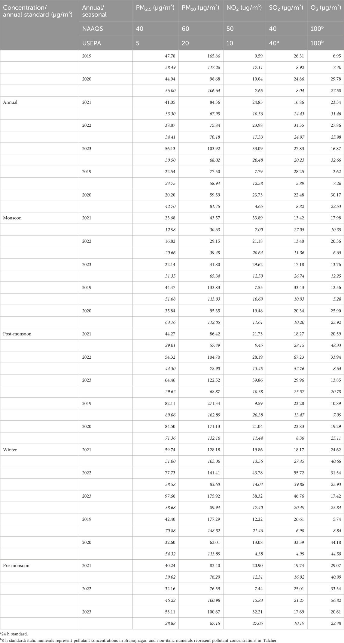
Table 1. Spatio-temporal concentrations (μg/m³) of criteria pollutants along with their regulatory standards.

4.2 Correlation between meteorological variables and criteria pollutants

Figure 3 illustrates the relationship between meteorological variables and criteria pollutants in Talcher and Brajrajnagar. In Talcher, precipitation has a poor correlation with PM_2.5 and PM₁₀, indicating wet deposition, as precipitation washes out PM during rainy seasons from the atmosphere, similar to the monsoon effect reported by Bozhkova et al. (2020) and Sharma et al. (2025). RH has a positive correlation, which suggests that high humidity promotes the hygroscopic growth of particles, leading to higher PM concentrations. WS has a moderate correlation (R = 0.36 for PM_2.5 and R = 0.33 for PM₁₀), suggesting that higher wind speeds facilitate pollutant dispersion. Temperature has a weak positive correlation with PM, suggesting that higher temperatures increase photochemical activity; therefore, the formation of secondary pollutants occurs (Kumar et al., 2022). In Brajrajnagar, precipitation shows a similar correlation with PM as in Talcher, but weaker, indicating lower precipitation efficacy in particle removal due to regional meteorological differences. RH and WS have a good positive correlation with precipitation and temperature, showing a weak positive correlation compared to Talcher, possibly due to differences in emission sources and local meteorological conditions.

Figure 3

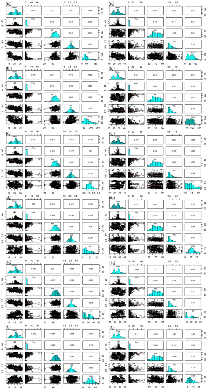
Figure 3. Meteorological correlation with criteria pollutants at Talcher (a₁–f₁) and Brajrajnagar (a₂–f₂).

In both stations, CO shows minimal reduction with precipitation due to its gaseous nature and low solubility. Temperature showed a good positive correlation, RH depicted a weak positive correlation, while WS showed a poor correlation with CO. NO₂ also depicts a poor correlation with precipitation and WS in both the stations. The positive correlation of temperature and RH may result from NO₂ accumulation under moist conditions, where dispersion is limited. The pollutant O₃ also exhibits similar correlations for both sites with all the meteorological variables. RH and WS showed a poor correlation with temperature, reflecting the role of temperature in accelerating photochemical reactions. The pollutant SO₂ also showed a poor correlation with precipitation, WS, and RH at both stations, indicating that SO₂ is effectively scavenged by rainfall, as noted in studies on industrial areas. However, temperature depicted positive correlations at both locations. The consistent WS and temperature trends confirm similar emission sources and meteorological influences. Positive correlations for PM and O₃ highlight the role of RH in promoting particle growth and photochemical activity. Temperature has positive correlations for most pollutants; particularly O₃ and NO₂ reflect the influence of temperature on emission rates and photochemical reactions.

4.3 Relative performance of machine learning ICR, ENET, and BT models

The ML performance metrics ICR, ENET, and BT were evaluated for both training and testing datasets using Taylor plots in Talcher and Brajrajnagar (Figures 4–6). Across both locations, the BT model consistently achieves higher R values, indicating better predictive accuracy for most of the pollutants. In Talcher, for PM_2.5 (training data), BT achieves R = 0.834, surpassing ICR (R = 0.748) and ENET (R = 0.748). For Brajrajnagar, BT also outperforms other models, particularly for CO (R = 0.519 in training) and SO₂ (R = 0.702 in training). The results are consistent with the findings reported by Gulia et al. (2022), demonstrating the superiority of BT in capturing complex relationships in air quality data.

Figure 4

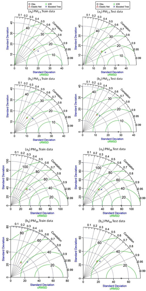
Figure 4. Comparative analysis of ICR, ENET, and BT models for training and testing data on PM_2.5 and PM₁₀ in Talcher (a₁–a₂) and Brajrajnagar (b₁–b₂) using a Taylor diagram.

Figure 5

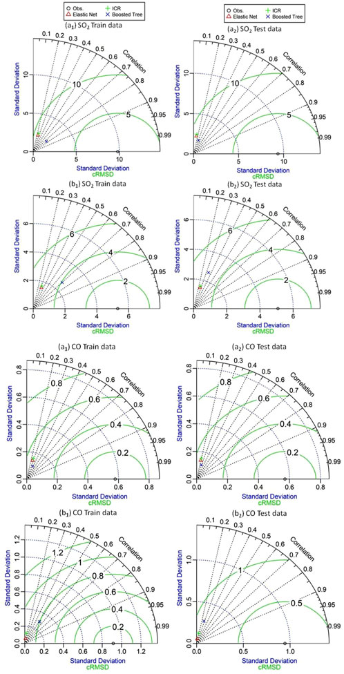
Figure 5. Comparative analysis of ICR, ENET, and BT models for training and testing data on SO₂ and CO in Talcher (a₁–a₂) and Brajrajnagar (b₁–b₂) using a Taylor diagram.

Figure 6

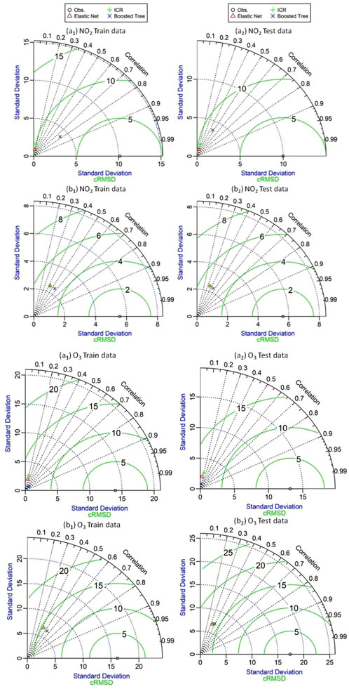
Figure 6. Comparative analysis of ICR, ENET, and BT models for training and testing data on NO₂ and O₃ in Talcher (a₁–a₂) and Brajrajnagar (b₁–b₂) using a Taylor diagram.

Table 2 summarizes the predictive performance of all three ML models for estimating PM_2.5, PM₁₀, CO, NO₂, O₃, and SO₂. The BT model demonstrates lower RMSE for most pollutants in both locations, suggesting improved model accuracy. In Talcher, PM_2.5 RMSE for training data is 16.799 (BT), compared to 20.157 (ICR) and 20.171 (ENET). In Brajrajnagar, the trend persists with the BT model, showing lower RMSE for PM_2.5 (19.277 vs 23.334 for ICR). These values are within the typical range reported in air quality modeling literature studies for regions with comparable pollution levels. PBias indicates the model’s tendency to overestimate or underestimate values. BT generally has lower PBias in both training and testing, reflecting fewer systematic errors. In Talcher, NO₂ (testing data) has a PBias value of 0.322 (BT) versus 4.853 (ICR). In Brajrajnagar, SO₂ (training data) shows a PBias value of −1.211 (BT), indicating closer alignment with observed values compared to −6.972 (ICR). This aligns with the recommendations of Willmott and Matsuura (2005), suggesting that a PBias value within ±10% is ideal for environmental modeling.

Table 2

Table 2. Statistical analysis between ICR, ENET, and BT models for Talcher and Brajrajnagar.

Models performed better overall in Talcher than in Brajrajnagar, with higher R values and lower RMSE. The BT model shows particularly strong performance for NO₂ and O₃, both pollutants of high interest due to their health impacts (World Health Organization, 2021). In Brajrajnagar, model performance, as indicated by lower R values and higher RMSE for certain pollutants like CO and NO₂, suggests greater variability or complexity in air quality data at this location. BT still remains the best-performing model but shows reduced efficacy compared to its performance in Talcher. This is consistent with studies that highlight challenges in areas with heterogeneous emission sources (Bozhkova et al., 2020). R values for pollutants such as PM_2.5 (0.834 in Talcher with BT) align with studies worldwide that often report R > 0.8 for well-performing models in air quality prediction. Lower R values for pollutants like CO in Brajrajnagar (R = 0.519) highlight challenges in modeling gases with more localized and transient sources. RMSE values for PM_2.5 and PM₁₀ are comparable to global benchmarks, where values typically range between 10 and 50 μg/m³, depending on regions and pollution levels (Gulia et al., 2022). For CO, RMSE values in the study (approximately 0.5–0.9 ppm) are consistent with other studies, indicating similar accuracy (Bozhkova et al., 2020). PBias values generally fall within acceptable limits (−10% to 10%), according to global standards for air quality model evaluation, although some exceptions exist, such as Brajrajnagar’s CO (Willmott and Matsuura, 2005). As anticipated, performance is typically better for the training dataset than the testing dataset, likely due to overfitting or the complexity of the model. Lower R values for CO and O₃ indicate that these pollutants are harder to predict accurately, possibly due to high variability in data for model training.

4.4 Assessment of the AQI and air pollutant trends

Figure 7 illustrates the annual trends of various air pollutants and the AQI for the locations of Talcher and Brajrajnagar during 2019–2023. In Talcher and Brajrajnagar, both pollutants PM_2.5 and PM₁₀ significantly decreased from 2019 to 2021, demonstrating improved air quality during these years. This significant decrease in PM was due to the COVID-19 lockdown. However, there is a slight increase observed between 2022 and 2023. PM_2.5 and PM₁₀ are the primary contributors to air quality degradation in both Talcher and Brajrajnagar. The AQI trends in both regions are closely linked to variations in PM levels, indicating that particulate matter is a critical determinant of air quality. NO₂ and SO₂ remain relatively stable throughout the time period, with minor fluctuations. O₃ levels are minimal, showing negligible variations across the years. The AQI followed the trend of PM₁₀ and PM_2.5, decreasing from 2019 to 2021 and slightly increasing from 2022 onward.

Figure 7

Figure 7. Variation in the AQI and key air pollutants in Talcher and Brajrajnagar during 2019–2023.

The annual mean AQI in Brajrajnagar depicted a progressive decrease year-by-year, with a stabilization observed between 2021 and 2023. Notably, the AQI showed a decreasing trend from 2019 to 2022, followed by a slight increase in 2023. In Brajrajnagar, NO₂ levels remain stable, while SO₂ is nearly negligible and shows no substantial changes. Ozone levels are relatively low, with no major seasonal or annual variability. The AQI decreases from 2019 to 2021 but increases slightly in 2023, mirroring the trend in particulate matter. NO₂, SO₂, and O₃ exhibit minimal variations, suggesting that these pollutants have a less significant impact on AQI in these locations.

4.5 Pollutant frequency of occurrence over coal mine complex belts

Figure 8 demonstrates the frequency of occurrence matrices by six subplots, each representing a specific pollutant: PM₂.₅, PM₁₀, NO₂, NOx, SO₂, and O₃. Brajrajnagar exhibits comparatively higher frequencies of days with PM_2.5 concentrations of 50 μg/m³ than Talcher. Talcher has a broader distribution with higher percentages and a higher frequency of days with elevated PM₁₀ concentrations, whereas Brajrajnagar shows a narrower distribution but a higher frequency of days with a concentration range of 100–200 μg/m³. This trend suggests comparatively higher industrial and coal-related activities in Talcher (Guttikunda and Jawahar, 2014). Both locations show similar trends for NO₂, with the highest percentage of days occurring at lower concentrations (0–40 μg/m³) However, the higher frequency of days is observed in the 20–30 μg/m³ and 40–60 μg/m³ ranges in Brajrajnagar and Talcher, respectively. NO_x also reported a comparatively higher frequency of days in Talcher (80–100 μg/m³), but at lower concentrations, NOx distribution was found more or less similar in both sites. Brajrajnagar has higher frequencies at lower SO₂ concentrations (0–30 μg/m³), while Talcher exhibits a higher proportion of days with elevated levels (40–100 μg/m³). SO₂ is a marker for emissions from coal combustion in power plants and industrial operations (Lelieveld et al., 2015). Talcher has a higher proportion of days with elevated SO₂ levels, justifying comparatively intense coal-based activities. Talcher appears to have higher O₃ concentrations (20–40 μg/m³) with high frequency, whereas Brajrajnagar shows a broad distribution range (50–100 μg/m³) with a higher frequency of days overall. O₃ is a secondary gaseous pollutant formed through photochemical reactions involving NO_x and VOCs (Seinfeld and Pandis, 2016). Talcher shows slightly higher O₃ concentrations, possibly due to higher precursor emissions and favorable atmospheric conditions.

Figure 8

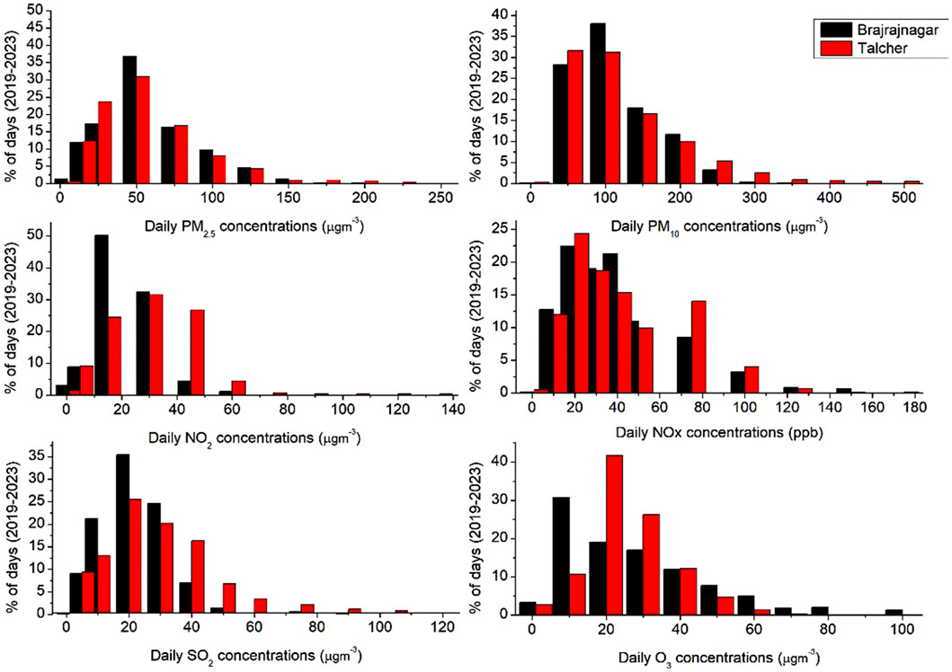
Figure 8. Comparing the frequency of daily criteria pollutant concentrations in Talcher and Brajrajnagar for the period of 2019–2023.

The frequency distribution indicates significant spatial variations in air quality due to local and regional anthropogenic sources and meteorological variability in the eastern coal mine complex. Talcher showed consistently higher pollutant concentrations across most metrics. A similar conclusion reported in prior studies indicates the role of industrial and mining activities in elevating air pollution levels in Talcher (Mishra and Das, 2017) compared to Brajrajnagar.

4.6 Correlation between the air quality index and health-based air quality index

Figure 9 demonstrates a comparative analysis of AQI and HAQI for two eastern coast coal mine complex stations from 2019 to 2023. The red dots signify upper bounds (HAQI_UB), and the black dots represent lower bounds (HAQI_LB). The spread of red dots indicates uncertainty in health impacts attributed to AQI levels. In Brajrajnagar, the AQI values tend to be lower overall than in Talcher, particularly in later years (2022 and 2023). However, HAQI values remain distributed, suggesting moderate air quality impacts on health. In Talcher, AQI values are more dispersed, with higher upper bounds observed in 2019 and 2020, correlating to larger HAQI variation. Across both regions, it was observed that at lower ranges, the AQI and HAQI demonstrate good correlation, but for higher ranges of concentration, the AQI underestimates the health risk severity. The year-wise variability demonstrated that in 2019, both regions showed higher AQI values, with Talcher reaching up to 350. In 2020, a slight reduction in AQI was observed in Brajrajnagar. However, Talcher maintains a higher range of AQI than Brajrajnagar. In 2021–2023, there was a steady decrease in AQI levels, with a corresponding stabilization of HAQI values, particularly in Brajrajnagar. Higher AQI levels in 2019 and 2020 align with potential public health concerns in Talcher, given the elevated HAQI and its bounds. The WHO highlights the relationship between air pollutants (as represented by AQI) and adverse health outcomes, which are reflected in the HAQI metric (World Health Organization, 2021). As outlined by Murray et al. (2015), HAQI captures the health-adjusted quality of life influenced by environmental, social, and behavioral factors, with air quality being a significant determinant. Previous studies on industrial areas, such as Talcher and Brajrajnagar, have documented the impact of industrial emissions on air quality and health outcomes (Sharma et al., 2020).

Figure 9

Figure 9. Correlation between the HAQI (lower and upper bound) and AQI for the years 2019–2023.

4.7 Comparative assessment of the AQI with the HAQI array

A comparative assessment of the AQI and HAQI, including their upper and lower boundaries, was performed to understand the health risks in two different indices across the two locations. Figure 10 represents the variability in AQI and HAQI with upper and lower bounds (HAQI_UB and HAQI_LB) during 2019–2023 for two locations. Shaded regions between HAQI_LB and HAQI_UB illustrate the range of variability in health risks due to air quality. The present study demonstrates that the AQI has increased over the years in both locations, signifying worsening air quality. HAQI values (both upper and lower bounds) increase over time for both locations, reflecting an increase in health risks from air pollution. The range between HAQI_LB and HAQI_UB is wider in Talcher. Talcher shows higher HAQI values (greater health risks) than Brajrajnagar across all years.

Figure 10

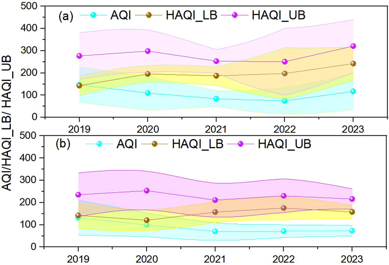
Figure 10. Variability in the AQI and HAQI with HAQI_UB and HAQI_LB in 2019–2023 for (a) Talcher and (b) Brajrajnagar. Shaded regions between HAQI_LB and HAQI_UB illustrate the range of variability in health risks due to air quality.

In the AQI, the health risk of exposure to criteria pollutants is based solely on the pollutant with the highest AQI value. However, in the HAQI, each sub-HAQI considers the RR due to multiple pollutants. Using the highest sub-HAQI as the overall HAQI provides a cautious approach to estimating multi-pollutant health risks, focusing on the pollutant with the greatest impact on health. When the AQI is ≤100, indicating healthy air quality, the HAQI aligns with the AQI, reflecting minimal health risk. Therefore, HAQI values should be considered an upper-bound estimate of health risks, reflecting the most harmful pollutant without inflating the overall risk. Although some studies aggregate various pollutants to estimate total risk, this study adopts the lower bound of the HAQI by calculating the combined impact of PM_2.5, O₃, SO₂, and NO₂, which is considered the lower bound for the HAQI. The comparison shows that multi-pollutant air pollution indices (HAQI) are elevated and pose significant health risks, while the AQI approach tends to underestimate these health risks.

4.8 Excessive risks over coal mine complex belts

Figure 11 demonstrates the percentage of ER for T and B, across criteria pollutants and ER_total from 2019 to 2023. Talcher consistently showed a higher ER than the Brajrajnagar region across the years for most pollutants, such as up to 6% higher risks for PM₁₀, 5% for NO₂, and up to 3% for SO₂. The trend in ER varies for different pollutants over the years. NO₂, PM₁₀, and PM_2.5 contribute significantly to the overall ER (Pathi et al., 2023). A number of previous studies highlighted the similar severity of industrial emissions on air quality and human health in coal mining and thermal power plant regions (Mishra and Das, 2017; Chowdhury and Paul, 2024). The findings enhance the understanding of air quality subtleties in industrial regions and offer crucial insights for policymakers and public health authorities to effectively mitigate potential health risks.

Figure 11

Figure 11. %ER due to criteria pollutants in Talcher (T) and Brajrajnagar (B) during 2019–2023.

5 Conclusion

The study highlights the critical role of ML models in estimating criteria pollutants and assessing their health risk in an industrialized coal mine and a thermal power plant region in eastern India. The analysis of time series trends, seasonal and annual spatio-temporal variations, and the percentage of days with poor air quality reveals significant spatial disparities in pollution levels. Talcher consistently demonstrates higher pollutant concentrations across most metrics, highlighting the substantial impact of industrial and mining activities on air quality with a broader frequency distribution of elevated levels for PM₁₀, NO₂, and SO₂ (>100 μg/m³, >40 μg/m³, and >40 μg/m³, respectively). In contrast, Brajrajnagar, despite its industrial activity, records comparatively lower pollutant levels. Talcher consistently records poorer AQI values with greater spatial variation. At lower AQI levels (good to satisfactory categories, AQI >100), both sites show minimal deviation. The BT model consistently demonstrated superior performance over ICR and ENET models in both Talcher and Brajrajnagar. However, results were found to be better, particularly in Talcher, which may be due to better input data and pollution source uniformity. The findings align with global standards, although localized variability in pollutants like CO and NO₂ indicates areas for improvement, such as incorporating additional predictors. This study highlights the importance of integrating ML with health risk assessments to develop effective, tailored mitigation measures for air pollution hotspots, advocating for targeted interventions to safeguard public health. ER analysis highlights health concerns, and Talcher shows greater health risks, with pollutant exposure up to 6% higher risks for PM₁₀, 5% for NO₂, and up to 3% for SO₂. These findings underscore the critical health implications of air quality disparities in these regions. The HAQI reveals that health risks are often underestimated by at least one category compared to the current AQI. The disparity between AQI and HAQI indicates that the AQI by itself does not adequately capture the health risks associated with exposure to multiple pollutants. Given these results, it is imperative for the public—particularly sensitive groups such as children, older adults, and individuals with lung or heart conditions—to adopt stricter measures to mitigate the adverse effects of air pollution. This need is especially urgent in highly polluted cities, hot spot areas, and during the winter season, when pollution levels peak.

Data availability statement

Publicly available datasets were analyzed in this study. These data can be found at: (https://app.cpcbccr.com/ccr/#/caaqm-dashboard-all/caaqm-landing/data).

Author contributions

PK: conceptualization, data curation, formal analysis, methodology, software, visualization, and writing – original draft. AC: conceptualization, data curation, formal analysis, visualization, and writing – original draft. PJ: writing – review and editing. RK: writing – review and editing. RB: conceptualization, resources, supervision, and writing – review and editing.

Funding

The author(s) declare that no financial support was received for the research and/or publication of this article.

Acknowledgments

The authors express their gratitude to NASA POWER for providing the meteorological data and CPCB, Govt. of India, for granting access to the criteria pollutant data. The authors (PK and AC) acknowledge the Raja Jwala Prasad (RJP) Post-Doctoral Fellowship (PDF) scheme, under the Institute of Imminence (IOE), BHU, Varanasi.

Conflict of interest

The author(s) declare that the research was conducted in the absence of any commercial or financial relationships that could be construed as a potential conflict of interest.

The handling editor CMA declared a past co-authorship with the author AC.

Generative AI statement

The author(s) declare that no Generative AI was used in the creation of this manuscript.

Publisher’s note

All claims expressed in this article are solely those of the authors and do not necessarily represent those of their affiliated organizations, or those of the publisher, the editors and the reviewers. Any product that may be evaluated in this article, or claim that may be made by its manufacturer, is not guaranteed or endorsed by the publisher.

References

Bozhkova, V. V., Liudchik, A. M., and Umreika, S. D. (2020). Influence of meteorological conditions on urban air pollution. Acta Geogr. Silesiana 14 (4), 5–21.

Google Scholar

Cairncross, E. K., John, J., and Zunckel, M. (2007). A novel air pollution index based on the relative risk of daily mortality associated with short-term exposure to common air pollutants. Atmos. Environ. 41, 8442–8454. doi:10.1016/j.atmosenv.2007.07.003

CrossRef Full Text | Google Scholar

Carty, D. M., (2011). An analysis of boosted regression trees to predict the strength properties of wood composites.

Google Scholar

Chang, J. C., and Hanna, S. R. (2005). Technical descriptions and evaluations of atmospheric dispersion models used in homeland security applications. J. Appl. Meteorol. 44 (4), 475–493.

Google Scholar

Choudhary, A., Kumar, P., Pradhan, C., Sahu, S. K., Chaudhary, S. K., Joshi, P. K., et al. (2023). Evaluating air quality and criteria pollutants prediction disparities by data mining along a stretch of urban-rural agglomeration includes coal-mine belts and thermal power plants. Front. Environ. Sci. 11, 1132159. doi:10.3389/fenvs.2023.1132159

CrossRef Full Text | Google Scholar

Choudhary, A., Kumar, P., Sahu, S. K., Pradhan, C., Joshi, P. K., Singh, S. K., et al. (2022). Health risk appraisal associated with air quality over coal-fired thermal power plants and coalmine complex belts of urban–rural agglomeration in the eastern coastal state of Odisha, India. ATM 13 (12), 2064. doi:10.3390/atmos13122064

CrossRef Full Text | Google Scholar

Chowdhury, I. R., and Paul, A. (2024). Respiratory health and air pollution in opencast coal mining region: a study in mahanadi coalfield Odisha, India. IEJ 72 (3), 460–476. doi:10.1177/00194662241235489

CrossRef Full Text | Google Scholar

Cohen, A. J., Ross Anderson, H., Ostro, B., Pandey, K. D., Krzyzanowski, M., Künzli, N., et al. (2005). The global burden of disease due to outdoor air pollution. J. Toxicol. Environ. Health A 68 (13-14), 1301–1307. doi:10.1080/15287390590936166

PubMed Abstract | CrossRef Full Text | Google Scholar

CPCB (2015). National air quality index report, central pollution control board. New Delhi, India.

Google Scholar

CPCB (2020). National ambient air quality standards, central pollution control board. New Delhi, India.

Google Scholar

Cropper, M., Gamkhar, S., Malik, K., Limonov, A., and Partridge, I. (2012). The health effects of coal electricity generation in India, Resources for the Future Discussion Paper.

Google Scholar

Das, P., Mandal, I., Pal, S., Mahato, S., Talukdar, S., and Debanshi, S. (2022). Comparing air quality during nationwide and regional lockdown in Mumbai Metropolitan City of India. Geocarto Int. 37 (25), 10366–10391. doi:10.1080/10106049.2022.2034987

CrossRef Full Text | Google Scholar

Diksha, D., Kumari, M., Mishra, V. N., Kumar, D., Kumar, P., and Abdo, H. G. (2024). Unveiling pollutants in Sonipat district, Haryana: exploring seasonal, spatial and meteorological patterns. Phys. Chem. Earth, Parts A/B/C 135, 103678. doi:10.1016/j.pce.2024.103678

CrossRef Full Text | Google Scholar

Elith, J., Leathwick, J. R., and Hastie, T. (2008). A working guide to boosted regression trees. J. Anim. Ecol. 77 (4), 802–813. doi:10.1111/j.1365-2656.2008.01390.x

PubMed Abstract | CrossRef Full Text | Google Scholar

Espitia-Perez, L., da Silva, J., Espitia-Perez, P., Brango, H., Salcedo-Arteaga, S., Hoyos-Giraldo, L. S., et al. (2018). Cytogenetic instability in populations with residential proximity to open-pit coal mine in Northern Colombia in relation to PM10 and PM2.5 levels. Ecotoxicol. Environ. Saf. 148, 453–466. doi:10.1016/j.ecoenv.2017.10.044

PubMed Abstract | CrossRef Full Text | Google Scholar

Friedman, J., Hastie, T., and Tibshirani, R. (2010). Regularization paths for generalized linear models via coordinate descent. J. Stat. Softw. 33 (1), 1–22. doi:10.18637/jss.v033.i01

PubMed Abstract | CrossRef Full Text | Google Scholar

Friedman, J. H. (2002). Stochastic gradient boosting. CSDA 38 (4), 367–378. doi:10.1016/s0167-9473(01)00065-2

CrossRef Full Text | Google Scholar

Gariazzo, C., Carlino, G., Silibello, C., Renzi, M., Finardi, S., Pepe, N., et al. (2020). A multi-city air pollution population exposure study: combined use of chemical-transport and random-Forest models with dynamic population data. Sci. Total Environ. 724, 138102. doi:10.1016/j.scitotenv.2020.138102

PubMed Abstract | CrossRef Full Text | Google Scholar

Gasparotto, J., and Martinello, K. D. B. (2021). Coal as an energy source and its impacts on human health. Energy Geosci. 2 (2), 113–120.

Google Scholar

GBD (2016). Global burden of disease study 2016 cancer incidence, mortality, years of life lost, years lived with disability, and disability-adjusted life years 1990–2016. Seattle, United States: Institute for Health Metrics and Evaluation IHME.

Google Scholar

Greenstone, M., and Jack, B. K. (2015). Envirodevonomics: a research agenda for an emerging field. JEL 53 (1), 5–42. doi:10.1257/jel.53.1.5

CrossRef Full Text | Google Scholar

Gulia, S., Shukla, N., Padhi, L., Bosu, P., Goyal, S. K., and Kumar, R. (2022). Evolution of air pollution management policies and related research in India. Environ. Challenges 6, 100431. doi:10.1016/j.envc.2021.100431

CrossRef Full Text | Google Scholar

Gupta, A., and Spears, D. (2017). Health externalities of India's expansion of coal plants: evidence from a national panel of 40,000 households. JEEM 86, 262–276. doi:10.1016/j.jeem.2017.04.007

PubMed Abstract | CrossRef Full Text | Google Scholar

Guttikunda, S. K., and Jawahar, P. (2014). Atmospheric emissions and pollution from the coal-fired thermal power plants in India. Atmos. Environ. 92, 449–460. doi:10.1016/j.atmosenv.2014.04.057

CrossRef Full Text | Google Scholar

Guttikunda, S., Jawahar, P., and Goenka, D. (2015). Regulating air pollution from coal-fired power plants in India. E.P.W. 1, 62–67.

Google Scholar

Hu, J., Ying, Q., Wang, Y., and Zhang, H. (2015). Characterizing multi-pollutant air pollution in China: comparison of three air quality indices. Environ. Int. 84, 17–25. doi:10.1016/j.envint.2015.06.014

PubMed Abstract | CrossRef Full Text | Google Scholar

Hyvärinen, A. (1999). Fast and robust fixed-point algorithms for independent component analysis. IEEE Trans. Neural Netw. 10 (3), 626–634. doi:10.1109/72.761722

PubMed Abstract | CrossRef Full Text | Google Scholar

Hyvärinen, A., Karhunen, J., and Oja, E. (2001). Independent component analysis. John Wiley and Sons.

Google Scholar

Kaneko, H., Arakawa, M., and Funatsu, K. (2008). Development of a new regression analysis method using independent component analysis. J. Chem. Inf. Model. 48 (3), 534–541. doi:10.1021/ci700245f

PubMed Abstract | CrossRef Full Text | Google Scholar

Kumar, P., Kapur, S., Choudhary, A., and Singh, A. K. (2022). Spatiotemporal variability of optical properties of aerosols over the Indo-Gangetic Plain during 2011–2015. Ind. J. Phys. 96, 329–341. doi:10.1007/s12648-020-01987-x

CrossRef Full Text | Google Scholar

Kumar, P., Pratap, V., Kumar, A., Choudhary, A., Prasad, R., Shukla, A., et al. (2020). Assessment of atmospheric aerosols over Varanasi: physical, optical and chemical properties and meteorological implications. J. Atmos. Solar-Terrest. Phy. 209, 105424. doi:10.1016/j.jastp.2020.105424

CrossRef Full Text | Google Scholar

Kumar, R. P., Singh, R., Kumar, P., Kumar, R., Nahid, S., Singh, S. K., et al. (2024). Aerosol-PM2. 5 Dynamics: in-situ and satellite observations under the influence of regional crop residue burning in post-monsoon over Delhi-NCR, India. Environ. Res. 255, 119141. doi:10.1016/j.envres.2024.119141

PubMed Abstract | CrossRef Full Text | Google Scholar

Lelieveld, J., Evans, J., Fnais, M., Giannadaki, D., and Pozzer, A. (2015). The contribution of outdoor air pollution sources to premature mortality on a global scale. Nature 525, 367–371. doi:10.1038/nature15371

PubMed Abstract | CrossRef Full Text | Google Scholar

Li, Q., Li, L., and Zhu, X. (2020). ElasticNet in financial forecasting: a comparison with Ridge and LASSO regression. QFE 4 (2), 456–469.

Google Scholar

Liu, H., Li, Q., Yu, D., and Gu, Y. (2019). Air quality index and air pollutant concentration prediction based on machine learning algorithms. Appl. Sci. 9 (19), 4069. doi:10.3390/app9194069

CrossRef Full Text | Google Scholar

Linard, C., Tatem, A. J., and Gilbert, M. (2013). Modelling spatial patterns of urban growth in Africa. Appl. Geogr. 44, 23–32. doi:10.1016/j.apgeog.2013.07.009

PubMed Abstract | CrossRef Full Text | Google Scholar

Lu, C. J., Lee, T. S., and Chiu, C. C. (2009). Financial time series forecasting using independent component analysis and support vector regression. Decis. Support Syst. 47 (2), 115–125. doi:10.1016/j.dss.2009.02.001

CrossRef Full Text | Google Scholar

Lu, F., Yuan, Y., Hong, F., and Hao, L. (2023). Spatiotemporal variations and trends of air quality in major cities in Guizhou. Front. Environ. Sci. 11, 1254390. doi:10.3389/fenvs.2023.1254390

CrossRef Full Text | Google Scholar

Main, A. R., Michel, N. L., Headley, J. V., Peru, K. M., and Morrissey, C. A. (2015). Ecological and landscape drivers of neonicotinoid insecticide detections and concentrations in Canada's prairie wetlands. Environ. Sci. Technol. 49, 8367–8376. doi:10.1021/acs.est.5b01287

PubMed Abstract | CrossRef Full Text | Google Scholar

Mishra, N., and Das, N. (2017). Coal mining and local environment: a study in Talcher coalfield of India. Air Soil Water Res. 10, 117862211772891. doi:10.1177/1178622117728913

CrossRef Full Text | Google Scholar

Müller, D., Leitão, P. J., and Sikor, T. (2013). Comparing the determinants of cropland abandonment in Albania and Romania using boosted regression trees. Agric. Syst. 117, 66–77. doi:10.1016/j.agsy.2012.12.010

CrossRef Full Text | Google Scholar

Murray, C. J., Barber, R. M., Foreman, K. J., Ozgoren, A. A., Abd-Allah, F., Abera, S. F., et al. (2015). Global, regional, and national disability-adjusted life years (DALYs) for 306 diseases and injuries and healthy life expectancy (HALE) for 188 countries, 1990–2013: quantifying the epidemiological transition. lancet 386 (10009), 2145–2191. doi:10.1016/s0140-6736(15)61340-x

PubMed Abstract | CrossRef Full Text | Google Scholar

Oberschelp, C., Pfister, S., Raptis, C. E., and Hellweg, S. (2019). Global emission hotspots of coal power generation. Nat. Sustain. 2 (2), 113–121. doi:10.1038/s41893-019-0221-6

CrossRef Full Text | Google Scholar

Oliveira, M. L. S., da Boit, K., Pacheco, F., Teixeira, E. C., Schneider, I. L., Crissien, T. J., et al. (2018). Multifaceted processes controlling the distribution of hazardous compounds in the spontaneous combustion of coal and the effect of these compounds on human health. Environ. Res. J. 160, 562–567. doi:10.1016/j.envres.2017.08.009

PubMed Abstract | CrossRef Full Text | Google Scholar

Pan, Y., Chen, S., Qiao, F., Ukkusuri, S. V., and Tang, K. (2019). Estimation of real-driving emissions for buses fueled with liquefied natural gas based on gradient boosted regression trees. Sci. Total Environ. 660, 741–750. doi:10.1016/j.scitotenv.2019.01.054

PubMed Abstract | CrossRef Full Text | Google Scholar

Patel, S., and Sharma, M. (2022). Evaluating the effectiveness of air pollution control policies: a case study of regulatory interventions. Front. Environ. Sci. 10, 89.

Google Scholar

Pathi, S. R., Dalai, B., Dash, S. K., and Agarwal, P. C. (2023). Air pollution in the industrial belts of Odisha: its health impacts with mitigation measures. J. Chem. Health Risks 13 (4), 214–227.

Google Scholar

Pratap, V., Kumar, A., Tiwari, S., Kumar, P., Tripathi, A. K., and Singh, A. K. (2020). Chemical characteristics of particulate matters and their emission sources over Varanasi during winter season. J. Atmos. Chem. 77, 83–99. doi:10.1007/s10874-020-09405-6

CrossRef Full Text | Google Scholar

Rajput, P., Sharma, P., and Gupta, A. (2022). Impact of firecracker bursting and long-range transport on PM₂.₅ concentrations in Kanpur during diwali. Front. Environ. Sci. 10, 858060.

Google Scholar

Rovira, J., Schuhmacher, M., Nadal, M., and Domingo, J. L. (2019). Contamination by coal dust in the neighborhood of the Tarragona Harbor (Catalonia, Spain): a preliminary study. Open Atmos. Sci. J. 12, 14–20. doi:10.2174/1874282301812010014

CrossRef Full Text | Google Scholar

Sahu, S. K., and Kota, S. H. (2017). Significance of PM2.5 air quality at the Indian capital. AAQR 17 (2), 588–597. doi:10.4209/aaqr.2016.06.0262

CrossRef Full Text | Google Scholar

Saini, P., and Sharma, M. (2020). Cause and age-specific premature mortality attributable to PM2.5 exposure: an analysis for million-plus Indian cities. Sci. Total Environ. 710, 135230. doi:10.1016/j.scitotenv.2019.135230

PubMed Abstract | CrossRef Full Text | Google Scholar

Salazar-Ruiz, E., Ordieres, J. B., Vergara, E. P., and Capuz-Rizo, S. F. (2008). Development and comparative analysis of tropospheric ozone prediction models using linear and artificial intelligence-based models in Mexicali, Baja California (Mexico) and Calexico, California (US) comparative analysis of tropospheric ozone prediction models using linear and artificial intelligence-based models in Mexicali, Baja California (Mexico) and Calexico, California (US). Environ. Model. Softw. 23 (8), 1056–1069. doi:10.1016/j.envsoft.2007.11.009

CrossRef Full Text | Google Scholar

Sayegh, A., Tate, J. A., and Ropkins, K. (2016). Understanding how roadside concentrations of NOx are influenced by the background levels, traffic density, and meteorological conditions using boosted regression trees. Atmos. Environ. 127, 163–175. doi:10.1016/j.atmosenv.2015.12.024

CrossRef Full Text | Google Scholar

Seinfeld, J. H., and Pandis, S. N. (2016). Atmospheric chemistry and physics: from air pollution to climate change. Hoboken: John Wiley and Sons.

Google Scholar

Shabani, F., Kumar, L., and Solhjouy-Fard, S. (2017). Variances in the projections, resulting from CLIMEX, boosted regression trees and random forests techniques. Theor. Appl. Climatol. 129, 801–814. doi:10.1007/s00704-016-1812-z

CrossRef Full Text | Google Scholar

Sharma, P., Singh, A., and Pandey, P. (2020). Impact of industrial emissions on ambient air quality and associated health risks: a case study of Talcher and Brajrajnagar industrial areas. J. Environ. Manage. 259, 110011.

Google Scholar

Sharma, V., Ghosh, S., Mishra, V. N., and Kumar, P. (2025). Spatio-temporal Variations and Forecast of PM2.5 concentration around selected Satellite Cities of Delhi, India using ARIMA model. Phys. Chem. Earth, Parts A/B/C, Parts A/B/C 138, 103849. doi:10.1016/j.pce.2024.103849

CrossRef Full Text | Google Scholar

Sicard, P., Talbot, C., Lesne, O., Mangin, A., Alexandre, N., and Collomp, R. (2012). The aggregate risk index: an intuitive tool providing the health risks of air pollution to health care community and public. Atmos. Environ. 46, 11–16. doi:10.1016/j.atmosenv.2011.10.048

CrossRef Full Text | Google Scholar

Singh, A., Verma, P., and Kumar, R. (2021). Impact of industrial emissions and meteorological factors on air quality trends in urban areas. Front. Environ. Sci. 9, 112.

Google Scholar

Stieb, D. M., Burnett, R. T., Smith-Doiron, M., Brion, O., Shin, H. H., and Economou, V. (2008). A new multipollutant, no-threshold air quality health index based on short-term associations observed in daily time-series analyses. JA&WMA 58, 435–450. doi:10.3155/1047-3289.58.3.435

PubMed Abstract | CrossRef Full Text | Google Scholar

Tong, D., Zhang, R., and Li, Y. (2021). Application of independent component regression in atmospheric pollution modeling. Environ. Model. Softw. 136, 104948.

Google Scholar

Wang, X., Zhang, K., Han, P., Wang, M., Li, X., Zhang, Y., et al. (2024). Application of gene expression programing in predicting the concentration of PM2.5 and PM10 in Xi’an, China: a preliminary study. Front. Environ. Sci. 12, 1416765. doi:10.3389/fenvs.2024.1416765

CrossRef Full Text | Google Scholar

Westad, F. (2005). Independent component analysis and regression applied on sensory data. J. Chemom. 19 (3), 171–179. doi:10.1002/cem.920

CrossRef Full Text | Google Scholar

Willmott, C. J., and Matsuura, K. (2005). Advantages of PBias in environmental modeling. Int. J. Climatol.

Google Scholar

Wong, T. W., Tam, W. W. S., Yu, I. T. S., Lau, A. K. H., Pang, S. W., and Wong, A. H. S. (2013). Developing a risk-based air quality health index. Atmos. Environ. 76, 52–58. doi:10.1016/j.atmosenv.2012.06.071

CrossRef Full Text | Google Scholar

World Health Organization (WHO) (2021). Ambient air pollution: a global assessment of exposure and burden of disease. Geneva, Switzerland: World Health Organization.

Google Scholar

Zou, H., and Hastie, T. (2005). Regularization and variable selection via the elastic net. J. R. Stat. Soc. Ser. B 67 (2), 301–320. doi:10.1111/j.1467-9868.2005.00503.x

CrossRef Full Text | Google Scholar