Comparative analysis of inflow forecasting using machine learning and statistical techniques: case study of Mangla reservoir and Marala Headworks

This study, under the context of a global perspective, focuses on the Indus Basin Irrigation System (IBIS) of Pakistan specifically the Jhelum and Chenab rivers inflows. The IBIS operation relies on seasonal planning strategies, informed by forecasts of river inflows at key stations by the Indus River System Authority (IRSA). In this study, Artificial Intelligence (AI) models including Generalized Regression Neural Network (GRNN), and Multi-Layer Feedforward Neural Network (MLFN) along with the statistical model Autoregressive Integrated Moving Average (ARIMA) were used to forecast the inflows of both rivers for 5 years (2020–2024) with a lead time of 1 year. Historic flow data of 59 years (10 daily from 1966 to 2024) were collected from IRSA. The collected data from 1966 to 2014 are used for calibration/training and from 2015 to 2020 are used for validation/testing of selected models for both study locations. The results of correlation and error estimation depicted that Artificial Neural Network (ANN) models predicted better inflows than the ARIMA model. The average RMSE and R² of ANN models is 9.68 and 0.92 and the average RMSE and ${\mathrm{R}}^2$ of ARIMA Model is 10.17 and 0.88, this results in improvement of average RMSE and ${\mathrm{R}}^2$ by 4.82% and 4.35% in case of ANN Models when compared with ARIMA Model. Qualitative analysis shows that ANN techniques better predicted the high and low flows when compared with statistical methods. Specifically, the application of the ANN models has enhanced the precision of forecasted inflows assessment compared to the probabilistic inflow forecasting methods used by IRSA. The average RMSE and ${\mathrm{R}}^2$ in case of IRSA forecast is 11.47 and 0.88 and the average RMSE and ${\mathrm{R}}^2$ in case of ANN Models is 10.30 and 0.92, this results in improvement of average RMSE and ${\mathrm{R}}^2$ by 10.20% and 4.35% in case of ANN Models when compared with IRSA forecast. This study highlights the need for utilization of ANN models in place of probabilistic inflow forecasting methods to improve the accuracy of time series inflow forecasts.

1 Introduction

Management of water resources is a universal challenge, transcending geographical boundaries. It has been in the limelight for decades due to climate and environmental changes at the global level. The increasing demand for water from various competing sectors also puts stress on available water resources, particularly in developing countries. In the case of shared river basins, the effective management of water resources is a key factor for optimal resource utilization (Agnihotri et al., 2022; Araghinejad et al., 2006; Danandeh Mehr et al., 2015). Indus Basin Irrigation System (IBIS) is one of the shared river basins, that flows through territories of India and Pakistan (Briscoe and Qamar, 2006). In the year 1960, to resolve the interstate water conflicts between two countries World Bank passed a treaty known as the Indus Water Treaty. According to the treaty, complete water rights of western rivers (Indus, Jhelum, and Chenab) are given to Pakistan, and rights of eastern rivers (Ravi, Sutlej, and Beas) are given to India (Ahmad et al., 2023). In Pakistan IBIS operates through intensive river control structures including dams, barrages, headworks, and interlinked canals to fully utilize the water potential of western rivers. However, to avoid inter-provincial conflicts regarding water distribution (Ahmad et al., 2021; Podger et al., 2021), the IRSA was established in the year 1992. IRSA is responsible for monitoring and regulating the IBIS within Pakistan and the distribution of water shared among provinces following the Water Apportionment Accord 1991 (Ahmad et al., 2023). The authority operates the IBIS on seasonal strategies, based on river inflows forecast at rim stations using probabilistic methods. It is based on the respective previous season inflow volume as an indicator of forthcoming season inflows. Therefore, to make informed decisions and equitable water sharing among provinces, precise inflow forecasting at rim stations is essential for avoiding conflicts and enhancing the optimal use of water resources.

Accurate stream flow forecasting is a challenging process due to its non-linear and multidimensional dynamics (Oyerinde et al., 2017; Rauf and Ghumman, 2018; Remesan et al., 2010). Numerous studies forecasted river inflow series through machine learning techniques, but the extent of forecast accuracy plays a vital role in the selection of specific techniques for a station. In literature, the flow prediction process is broadly divided into two types, namely, data-driven and physical base modeling approaches (Hassan and Hassan, 2021; Wang et al., 2006; Yaseen et al., 2018). Physical-based modeling approaches are complex but have the advantage of incorporating physical observations during prediction, however extracting accurate physical information of the river watersheds is not simple (Hassan and Hassan, 2021; Zhang et al., 2015). The data-driven methods majorly depend on the input and output data features instead of physical-based processes (Cui et al., 2020; Hassan et al., 2015). In data-driven methods, a variety of input data combinations (river stage, precipitation, temperature, and evaporation, etc.) can be used coupled with main input data variables (Jajarmizadeh et al., 2015; Wang et al., 2006). Many researchers have used the combination of three input parameters, namely, precipitation, temperature, and flow as reported in the literature. However, a commonly used combination by the researchers consists of precipitation and flow data together (Rauf et al., 2018).

A limited number of studies have used the single input data of flow in their research (Danandeh Mehr et al., 2015; Yaseen et al., 2018). The accuracy of traditional data-driven methods for flow prediction is quite reasonable (Rauf et al., 2018; Awchi, 2014). Traditional models include the Autoregressive (AR), the Autoregressive Moving Average (ARMA), the Autoregressive Integrated Moving Average (ARIMA) models, the probabilistic method, Support Vector Machine (SVM), and Random Forest (RF) (Nguyen et al., 2022). These methods are simple and unable to capture the complex relationships and on the other hand, the hydrological process that occurs in the watershed is a non-linear and complex phenomenon. Therefore, to increase the accuracy of flow prediction, non-linear models are necessary to accurately capture the intricate connections among observed data.

In recent years, deep learning methods based on Artificial Intelligence (AI) gained popularity among researchers, primarily for their effectiveness in mastering non-linear hydrological data behaviors and delivering high accuracy in prediction (Kisi and Sanikhani, 2015; Nguyen et al., 2022; Uysal et al., 2016). Various deep learning methods like Artificial Neural Network (ANN), Long Short-Term Memory (LSTM), Convolutional Neural Network (CNN), Multilayer Perceptron (MLP), Bidirectional Long Short-Term Memory (STM), Support Vector Classifier (SVC), Support Vector Regression (SVR), Adaptive Neuro-Fuzzy Inference System (ANFIS), Radial Basis Function (RBF), Feedforward Neural Networks (FFNN), General Regression Neural Network (GRNN) and MLFN have been adopted by various researchers with various input combinations (Afan et al., 2020; Cheng et al., 2020; Chu et al., 2021; Ibrahim et al., 2022; Khosravi et al., 2020; Kovačević et al., 2018; Le et al., 2019; Li et al., 2020; Rasouli et al., 2012; Wang et al., 2006).

Several existing research studies have integrated these techniques with various methods to enhance prediction accuracy (Nguyen et al., 2022). Pan et al. (2020) combined the CNN and GA to enhance the prediction accuracy of water level in the Yangtze River. Shiri et al. (2016) utilized the Extreme Learning Machines (ELM) approach to forecast the daily water level of Urmia Lake.

Choi et al. (2020) integrated ANN, RF, decision tree (DT), and SVM to predict the water level in South Korea. Nguyen et al. (2022) combine the three techniques LSTM, CNN, and Singular-spectrum analysis (SSA) to predict discharge and water level at two hydrological stations, Son Tay and Kon Tum, Vietnam. The author highlighted that predicting the discharge and water level is challenging due to several fundamental issues including short-term data for training and different hydrological behavior of each watershed in terms of runoff.

Previous studies have shown that only a limited number of research efforts have focused on predicting flow using a single input variable. In addition to a few studies using single input variables, the literature reveals a diverse range of data-driven methods and integrated techniques to predict flows. The justification for using single input variable of flow for inflow forecasting are the following.

1. Historic river inflow data shows strong temporal correlation.

2. The inflows capture Catchment response.

3. The inflows are recorded through accurate gauging stations and the data is reliable.

The involvement of multiple variables as in case of rainfall-runoff modeling for inflow forecasting would require complex computations specifically when are dealing with huge catchment area associated with Mangla and Marala Catchments. Moreover, the application of the MLFN method has not been explored for flow prediction with a single input variable. Therefore, in this study, inflow forecasting for Mangla Dam situated at River Jhelum, and for Marala Headworks located at Chenab River has been carried out using a statistical model (ARIMA) and artificial neural network models (GRNN and MLFN) and models’ performance has been investigated to select the best model at the individual study location. Further, a comparison has been made between the forecasted results of selected models with the forecasted inflows of the probability method adopted by IRSA, Pakistan. Utilizing the advanced methods helps to understand the strengths and limitations of each model, ultimately guiding future improvements in inflow prediction and model selection for better water resource management.

2 Study area and data set

This study is carried out for Mangala Dam and Marala Headworks located within the world largest contiguous irrigation network called as Indus River System. In Pakistan, the Indus River System consists of seven major rivers: Kabul, Indus, Jhelum, and Chenab are located on the western side, and Ravi, Sutlej, and Beas located on the eastern side. This largest system is regulated through three major reservoirs (Tarbela, Mangla, and Chashma), 15 barrages, 45 main canals, and inter-river link canals to utilize 130 billion m³ (BCM) of river water annually. The selected study locations play a vital role in the water resource management of the country throughout the year, as shown in Figure 1.

Figure 1

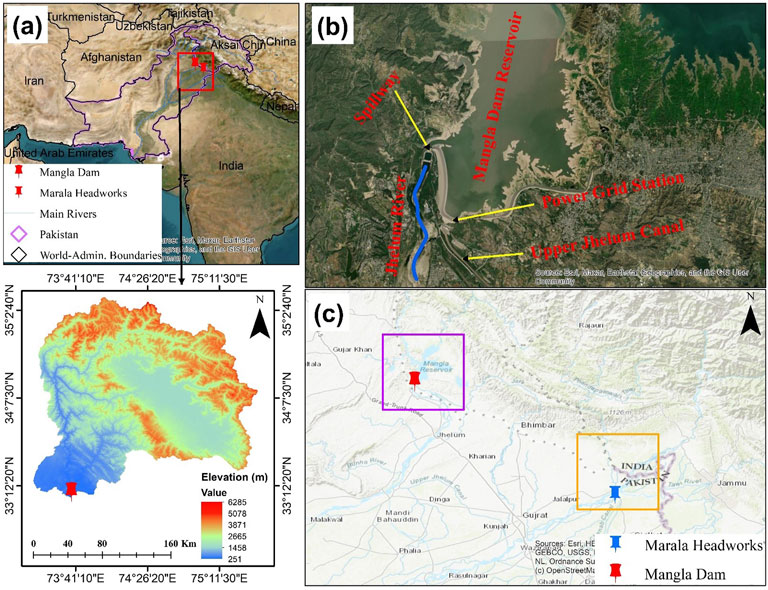
Figure 1. Political boundary of Pakistan with major rivers (a) and aerial photographs of study area locations; mangala dam (b) and marala headworks (c).

Geographically, Mangla Dam has a catchment area of 33,490 km² and is located at 33°08′31″N and 73°38′42″E. It regulates the flow of the Jhelum River and flows into the Chenab River at a confluence point upstream of Trimmu Headworks. Mangla Dam watershed area consists of seven sub-basins namely,: Neelum, Poonch, Upper-Jhelum, Kunhar, Kanshi, Lower Jhelum, and Kahan (Babur et al., 2016). The major portion of inflows in Mangla Dam are received from March to August and 25% of inflows are received in the rest of the months. Marala Headworks on the other hand located at 32°40′24″N and 74°27′50″E. It regulates the flow of Chenab, a transboundary river, and has a total catchment area of 67,430.34 ${\text{km}}^2$. At Marala Headworks 28,480.97 ${\text{km}}^2$ of catchment area contributes to the river flow after traveling a distance of 506 km (Ali et al., 2021). The inflows in the Chenab River are generated through snowmelt augmented by runoff from precipitation during monsoon.

Historic flow data of 59 years (10 daily from 1966 to 2024) were collected from IRSA. The ten daily flow data represents average flow data on 10 daily basis. The construction of Mangla Dam was completed in 1962 and IRSA started flow observation at Mangla Dam since 1966 onward. Therefore, historic flow data from 1966 onwards till 2024 was used at both of the study locations for the purpose of inflow forecasting. The flow patterns at both study locations during the stated period of historic flow data showed strong temporal correlation.

The collected data was averaged into twelve monthly flows for both study locations and plotted for comparative analysis. Figure 2 depicts the sessional inflow pattern at both study locations. Mangala station received the maximum inflows during March to August and Marala station received the maximum inflows during June to September.

Figure 2

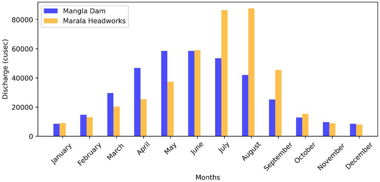
Figure 2. Mean monthly inflows at both study locations.

3 Methodology

Historic flow data was collected from the Indus River System Authority (IRSA) https://pakirsa.gov.pk/ and divided into various lengths for calibration, validation, training, and testing purposes. The flowchart of the methodology used in this study is presented in Figure 3.

Figure 3

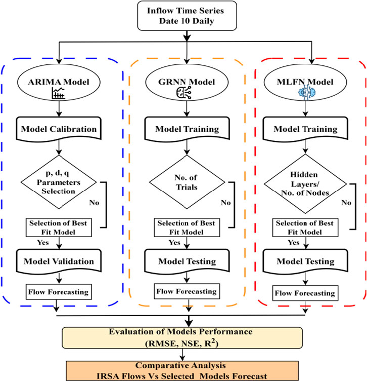
Figure 3. Flow Chart of methodology used in the present study for inflow forecasting.

Analysis of historic data was carried out for the identification of data nature and order of dependencies using the Autocorrelation Function (ACF) and Partial Autocorrelation Function (PACF). Both functions play a vital role in understanding the relationships within time series data and choosing appropriate parameters for the ARIMA model. The ACF measures the correlation between a time series and lagged values, moreover, detects repeating patterns like seasonality and determines the order of moving average (MA) component. The PACF assesses the direct impact of each lag by eliminating the influence of intermediate lags, moreover, helps to identify the order of autoregressive (AR) component. The mathematical form of equations used for determination of ACF for a given value of a lag “k” is given in Equation 1 and for calculation of PACF at varying lags (2^nd and 3^rd order) are given in Equation 2 and Equation 3.

$\text{ACF}=\frac{{\displaystyle {\sum }_{t=k+1}^T}\left(X_t-\overline{X}\right)\left(X_{t-k}-\overline{X}\right)}{{\displaystyle {\sum }_{t=1}^T}\left(X_t-\overline{X}\right)}(1)$

${\text{PACF}}_2=\frac{Covariance\left(x_t,x_{t-2}|x_{t-1}\right)}{\sqrt{Variance\left(x_t|x_{t-1}\right)Variance\left(x_{t-2}|x_{t-1}\right)}}(2)$

${\text{PACF}}_3=\frac{Covariance\left(x_t,x_{t-3}|x_{t-1},x_{t-2}\right)}{\sqrt{Variance\left(x_t|x_{t-1},x_{t-2}\right)Variance\left(x_{t-3}|x_{t-1},x_{t-2}\right)}}(3)$

where X = time series data, k = lag. Figure 4 drawn between, ACF with corresponding lag is called auto-correlogram and PACF with corresponding lag is partial auto-correlogram. The comparative auto-correlogram of the historic inflow series (1966–2024) of Mangla Dam and Marala Headworks are shown in Figure 4. The auto-correlogram of both inflow time series depicts that autocorrelation is periodic and decreases slowly with damping peaks which indicates the non-stationarity of time series. Figure 4 illustrates the partial auto-correlogram of the historic inflow series (1966–2024) of both study locations and depicts that with increasing lag PACF does not remain constant which indicates the non-stationary nature of time series data. The historical inflow data revealed strong seasonality, we opted to use the ARIMA model rather than SARIMA. The justifications for opting the ARIMA model is as follows.

1. Model performance evaluation of ARIMA Model showed satisfactory results, indicating that the added complexity of SARIMA Model will not offer any significant improvement.

2. Furthermore, after applying appropriate transformations and differencing, the time series data achieved stationarity without the need for seasonal terms.

Figure 4

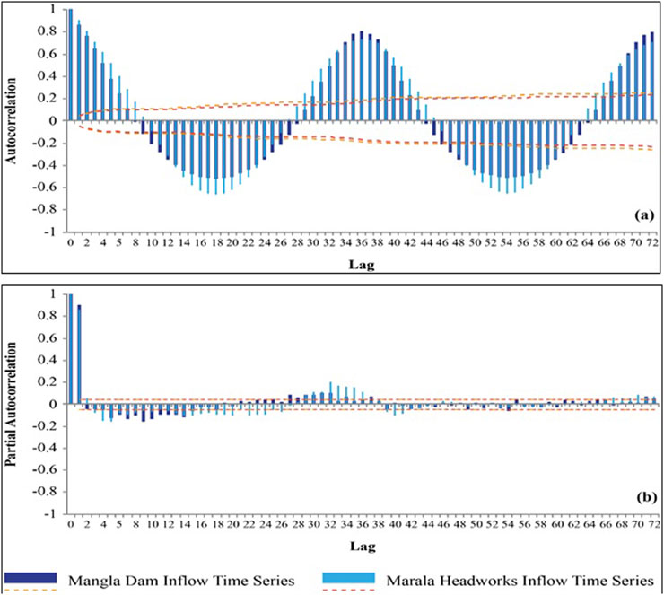
Figure 4. (a) Autocorrelogram (b) partial autocorrelogram, for mangla and marala inflows.

Therefore, ARIMA model parameters are selected accordingly to predict the inflow forecast.

3.1 ARIMA model

Various research studies discussed the detailed theory of ARIMA presented by (Box et al., 2015) and in this section, a brief overview is presented. The model’s name consists of three parts (a) AR (b) I and (c) MA. The “autoregressive (AR)” represents the use of lagged values of the differenced time series in the forecasting equations, capturing the influence of prior values on the current observation. The “integrated (I)” part signifies the need to differentiate the time series to make it stationary, ensuring that statistical properties remain consistent over time. The “moving average (MA)” component involves lagged forecast errors, accounting for the relationship between forecast errors and the observed data. It is simple to implement and effective for short-term forecasting, especially when dealing with stationary or moderately non-stationary time series (Wang et al., 2017; Yu et al., 2017). The general form of ARIMA (p, d, q) in backshift notation is given in Equation 4; denotation “p” represents the order of autoregressive (AR), “d” represents the order of differencing operator, and “q” represents the order of moving average (MA).

$\left(1-{ɸ}_{1}B-{ɸ}_2{B}^2-\dots \dots \dots .{ɸ}_p{B}^p\right){\nabla }^{d}X\left(t\right)=\left(1-{\theta }_{1}B-{\theta }_2{B}^2-\dots \dots \dots {\theta }_q{B}^q\right)\epsilon \left(t\right)(4)$

where: ${ɸ}_i$ = Autoregressive Coefficient, for i = (1, 2, 3, … , p), B = Backshift Operator. X (t) = nonstationary time series, ∇ = represents differencing operation, d = order of differencing, ε (t) = uncorrelated identically distributed error with zero mean, known as white noise., ${\theta }_i$ = Moving Average Parameter, for i = (1,2,3, … , q).

The significant parameter values of “p” and “q” are selected from ACF and PACF time series analysis shown in Figure 4. The value of the “d” parameters is selected after multiple trials to convert the non-stationary time series data to stationary time series.

3.2 General regression neural network (GRNN) model

This method is the type of artificial neural network (ANN) model that is particularly well-suited to predict time series values based on input time series. GRNN can handle non-linear relationships without iterative training and derive function directly from the training data (Kerem, 2005; Specht, 1991). Moreover, estimation error converges to zero with the increase of training data, imposing mild constraints on the function (Kerem, 2005). The fundamental idea behind GRNN is to model and reconstruct the underlying regression function Y(X), which defines the relationship between input variables and target outputs, using the information contained in the training data (Kopal et al., 2022). The Nadaraya–Watson kernel regression estimator used to predict the Y(X) for a single-bandwidth GRNN is given in Equation 5 (Pernot and Savin, 2020).

$Y\left(X\right)=\frac{{\displaystyle {\sum }_{i=1}^n}{Y}_i\exp \left(\frac{-{D_i}^2}{2{\sigma }^2}\right)}{{\displaystyle {\sum }_{i=1}^n}\exp \left(\frac{-{D_i}^2}{2{\sigma }^2}\right)}(5)$

Where

$D_i^2\left(X,X_i\right)={\displaystyle \sum _{k=1}^R}{‖X_k-X_{ik}‖}^2={\displaystyle \sum _{k=1}^R}{\left(X_k-X_{ik}\right)}^T\left(X_k-X_{ik}\right)(6)$

X = Input Sample, ${\mathrm{X}}_{\mathrm{i}}$ = Training Sample, ${\mathrm{Y}}_{\mathrm{i}}$ = Output of Input sample ${\mathrm{X}}_{\mathrm{i}}$, ${{\mathrm{D}}_{\mathrm{i}}}^2$ = Squared Euclidean distance between the training sample ${\mathrm{X}}_{\mathrm{i}}$ and input X, T = Matrix Transpose, Y = Estimated Output of the input sample X, σ = standard deviation.

Equation 5 and Equation 6 show that predicted values Y(X) are computed as a nonlinear weighted average of the target values Y_i associated with the training inputs X_i, where the weights are governed by the Gaussian radial basis function (RBF) as given in Equation 7.

${\psi }_i\left(X,X_i\right)=\exp \left(-\frac{D_i^2\left(X,X_i\right)}{2{\sigma }^2}\right)(7)$

The procedure adopted for predictor selection in the GRNN model involves following steps.

1. Normalization of predictors and handling of outliers and missing values.

2. Using filters to reduce dimensionality.

3. Measure GRNN performance with different feature subsets using suitable matrices (MAE, RMSE, etc.).

4. For feature selection the model applies forward or backward wrapper method.

5. Finally, the programme models the forecast for testing and training using selected predictors.

The architecture of the GRNN consists of four layers as shown in Figure 5. The input layer for incorporation of data. The second layer known as the pattern layer contains patterns that represent the learned patterns from data. The third layer of summation, the output of the pattern layer is the input of the summation layer which aggregates the information. The output layer generates the network’s predictions based on processed data from the summation layer (Kerem, 2005).

Figure 5

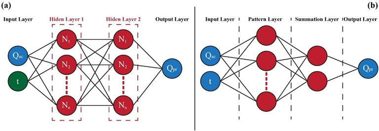
Figure 5. Schematics of (a) MLFN (b) GRNN.

3.3 Multilayered feedforward neural network (MLFN)

The MLFN is a type of artificial neural network and works on the principle of feedforward networks (Tayfur et al., 2007). It is structured with three primary components: (i) input layer, (ii) one or more hidden layers, and (iii) output layer, as shown in Figure 5. All the components are interconnected in a sequential, feedforward manner. The input layer neuron receives data and passes it to the first hidden layer neuron after multiplication with weight values. In case, multiple hidden layers are selected then each layer is sequentially connected with other hidden layers neurons, the output of the one layer serves the input of the subsequent layer. Moreover, hidden layer neurons process information of weighted inputs received from input layer neurons, perform bias correction, and transform the results using an activation function. The neurons in the output layer execute the same procedure and apply similar transformations to produce results (Chen and Leung, 2005). The weight-related equation used in MLFN with values function of n variables f (X₁, … , X_n) with n+1 complex-valued weight as parameters is shown in Equation 8.

$f\left(X_1,\dots ,X_n\right)=P\left(\left(W_0+W_1{X}_1+\dots +W_n{X}_n\right)+b_{l_1}\right)(8)$

where X = variable, W = weight, P = activation function, b = bias correction for layer.

In MLFN model each predictor appear as a node in the input layer and these nodes are connected to neurons in the hidden layers through weights. Then the leaning algorithm make adjustments in the weights to reduce the prediction error. The MLFN Model uses filter methods including ANOVA, Chi square test, Correlation method and Mutual Information method before training. Then the model itself evaluate the subset of predictors using the wrapper methods including backward elimination method, forward selection method and Recursive feature elimination method. During training of the model, the programme uses embedded methods including Regularization method, Drop out in neural netwroks and Permutation importance method.

3.4 Models performance evaluation

The evaluation of the model’s performance, during calibration/training, validation/testing, and forecasting stages, to assess their accuracy and reliability is one of the most important procedures. In literature, various statistical measures are adopted by various researchers to thoroughly assess the model performance. In this study, the following statistical indicators are used to assess the model’s goodness of fit.

3.4.1 Root mean square error (RMSE)

It represents the square root of the average of the squared difference between the predicted and observed data.

$\text{RMSE}=\sqrt{\frac{\sum {\left(X_0-X_f\right)}^2}{n}}(9)$

where, ${\mathrm{X}}_{\mathrm{f}}$ = Forecasted Values, ${\mathrm{X}}_{\mathrm{o}}$ = Observed Values

The higher the RMSE, indicates a greater discrepancy between the forecasted and observed values, and the lower the RMSE represents the better the model’s accuracy to predict.

3.4.2 Nash sutcliffe efficiency (NSE)

The model was first proposed by Nash and Sutcliffe and is one of the important statistical parameters used to indicate the model’s predictive accuracy.

$\text{NSE}=1-\frac{\sum {\left(X_o-X_f\right)}^2}{\sum {\left(X_o-\overline{X_o}\right)}^2}(10)$

The model accuracy indicators for NSE range from −1 to 1. A higher NSE value indicates a better model performance and a lower value indicates a worse performance. Value <0 indicates poor model predictive ability.

3.4.3 Coefficient of determination (R²)

R² is a statistical parameter that indicates the accuracy of model predictions by comparing the difference between observed and forecasted values in terms of average absolute deviation relative to the observed values.

${\mathrm{R}}^2=\frac{\sum \left({\mathrm{X}}_{\mathrm{o}}-\overline{{\mathrm{X}}_{\mathrm{o}}}\right)\left({\mathrm{X}}_{\mathrm{f}}-\overline{{\mathrm{X}}_{\mathrm{f}}}\right)}{\sqrt{\sum {\left({\mathrm{X}}_{\mathrm{o}}-\overline{{\mathrm{X}}_{\mathrm{o}}}\right)}^2\sum {\left({\mathrm{X}}_{\mathrm{f}}-\overline{{\mathrm{X}}_{\mathrm{f}}}\right)}^2}}(11)$

The value range of R² is between the values 0–1; higher model accuracy is indicated if the value nears 1 and bad model accuracy is indicated if the value is near zero.

4 Results

4.1 Models calibration, validations, training and testing

Historic flow data of 59 years were collected from IRSA. The collected data from 1966 to 2014 are used to calibration/training and from 2015 to 2020 are used for validation/testing of selected models for both study locations. We have used 49 years of historic flow data for calibration/training purpose which constitutes about 89% of the total length of historic flow data used. The calibration/training data length should be of sufficient length so as to get reliable forecasting results. We have used 6 years of historic flow data for validation/testing purpose which constitute about 11% of the total length of historic flow data used. The historic flow data from 1966 to 2024 were used for flow forecasting for the year 2020, 2021, 2022, 2023 and 2024 using lead time of 1 year and data of the last 5 years (2020–2024) were used for performance evaluation of the forecasted inflows for the year 2020–2024.

4.1.1 ARIMA model

The ARIMA model was calibrated and validated for the periods between 1966 to 2014 and 2015 to 2020 respectively for both study locations. The model was run with significant values of “p” and “q” as per the PACF and ACF analysis (shown in Figure 4), and varying values of difference operator “d”. The model performance was evaluated using the RMSE, NE, and R². Given the relatively low-dimensional parameter space and the interpretability of time series diagnostics, manual tuning based on statistical heuristics was sufficient and computationally efficient. Hence, exhaustive hyperparameter optimization was not necessary.

Table 1 shows the calibration and validation of the ARIMA model for Mangala Dam. Table 2 shows the calibration and validation of the ARIMA model for Marala Headworks. Multiple model scenarios were performed and evaluated, to select the best-fit model architecture and used for future forecasting of inflows. Varying combinations of “p”, “d” and “q” were tested ranging between 1–37, 0–1, and 1–30 respectively. The impact of various combinations in terms of model prediction accuracy was assessed and found that higher values in the case of p and q with difference operator (d) one (1) performed better as compared to lower values with d = 0. The detailed results are tabulated in Tables 1,2. The selected model 37, 1, 21 for Mangala Dam outperforms the other models’ scenarios during calibration with values of 9.0146, 0.8521 and 0.9231 for RMSE, NSE, and R² respectively. In the case of Marala Headworks, model 31, 1, 30 outperforms the other models’ scenarios during calibration with values of 13.8290, 0.8198, and 0.9055 for RMSE, NSE, and R² respectively. Moreover, these models were validated (2015–2020) for both study locations and results indicated improvement in the statistical performance indicators (Tables 1, 2).

Table 1

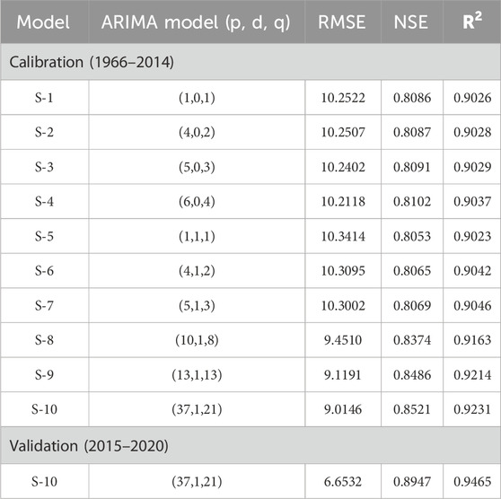
Table 1. Calibration and validation of ARIMA (p, d, q) model for Mangla Dam.

Table 2

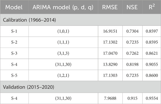
Table 2. Calibration and validations of ARIMA (p, d, q) model for Marala Headworks.

4.1.2 GRNN model

The model training and testing were carried out for both study locations. GRNN has relatively few hyperparameters, with the smoothing parameter (spread) being the primary one influencing performance. In our case, we selected the spread parameter using a trial-and-error approach combined with performance evaluation on a validation set. Due to the simple architecture and the model’s robustness to small variations in spread, hyperparameter optimization will not provide a significant advantage and was therefore not used.

In the training phase model was run with varying numbers of trials ranges 250,000 to 5,000,000. Tables 3, 4 show the training and testing of the GRNN model for Mangla Dam and Marala Headworks respectively. Multiple model iterations were performed and evaluated, to select the best fit model for future forecasting of inflows. We studied the impact of several iterations on model prediction accuracy and observed that in the case of Mangla Dam lesser iterations showed better model precision as compared to Marala Headworks which showed satisfactory results in the case of higher iterations. Moreover, this trend in iterations indicated the influence of seasonality in historic time series data during training as depicted in Figure 3. The selected model with iterations 250,000 for Mangala Dam (Table 3) and 5,000,000 for Marala Headworks (Table 4) outperforms the other models’ scenarios during training. The statistical indicators for selected models are 12.09 and 14.32 for RMSE, 0.7240 and 0.8050 for NSE, and 0.8511 and 0.8974 for R². Moreover, testing (2015–2020) of both selected models showed improved results regarding the statistical performance indicators (Tables 3, 4).

Table 3

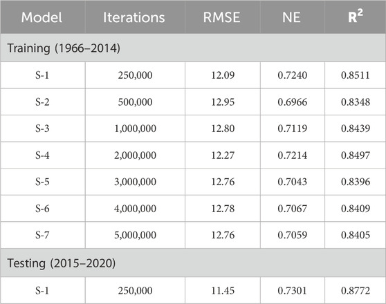
Table 3. Training and testing of GRNN model for Mangla Dam.

Table 4

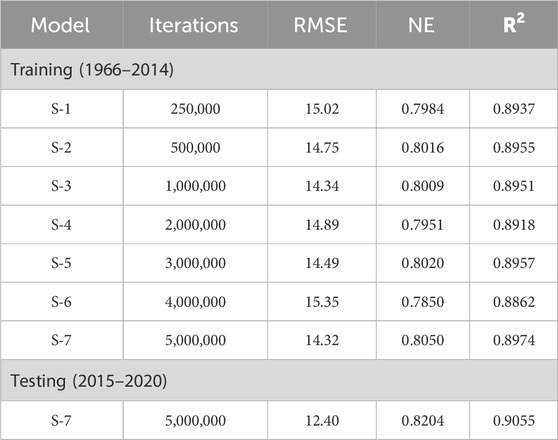
Table 4. Training and testing of the GRNN model for Marala Headworks.

4.1.3 MLFN model

The hyperparameter optimization in fuzzy systems as in MLFN Model can be computationally intensive with marginal gains, especially when the model already demonstrates acceptable performance, therefore hyperparameter optimization was not used.

Table 5, 6 presented the training of the MLFN model with a variety of combinations of hidden layers with varying numbers of nodes and testing of selected models for both stations. In the training phase model was run for hidden layers ranging from 1 to 2 and several nodes ranging from 2 to 10 in the respective hidden layers. Although multiple combinations were run, only the model scenarios with satisfactory results are presented in Tables 5, 6. The selected models based on statistical performance indicators are highlighted in these tables. In the case of Mangla Dam, the selected model with two layers coupled with 4 nodes in the first layer and 10 nodes in the second layer outperformed others with values of 12.54, 0.7168, and 0.8466 for RMSE, NSE, and R² respectively. For Marala Headworks, a selected model with two layers coupled with 2 nodes in each outperformed the other models’ combinations with values of 13.61, 0.8177, and 0.9043 for RMSE, NSE, and R² respectively. Moreover, testing (2015–2020) of both selected models showed satisfactory results.

Table 5

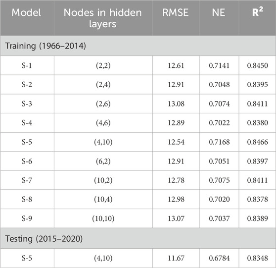
Table 5. Training and testing of the MLFN model for Mangla Dam.

Table 6

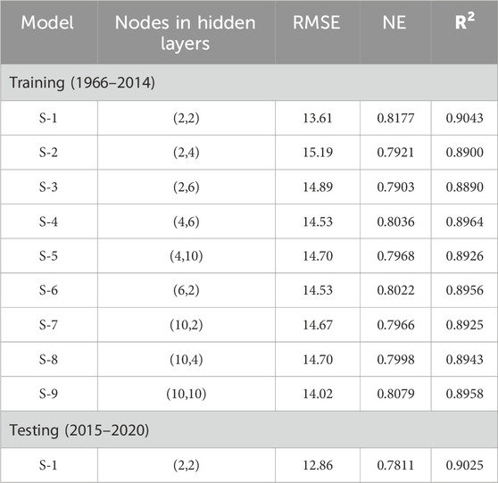
Table 6. Training and testing of the MLFN model for Marala Headworks.

4.2 Flow forecasting

Most of the forecasting models condition the forecast based on previous observations. Like in ARIMA you are predicting future values based on 1. Past observations (AR part) 2. Past forecast errors (MA part) and 3. Differenced values if the original data is not stationary. Similarly, the AI techniques also conditions on past observations while forecasting.

In this section, the prediction capabilities of the three selected models are assessed. The inflows at both stations were predicted for 5 years 2020–2024 with a lead time of 1 year. Moreover, the performance of each model was compared through statistical indicators, and analyzed the model’s output qualitatively. Based on the indicators and qualitative analysis results, the best-suited model for each study station was selected and their forecasted results were compared with the IRSA forecasted inflow time series.

4.2.1 Mangla dam station

To evaluate the prediction capability of ARIMA (37, 1, 21), GRNN (250,000), and MLFN (4.10), we compared the predicted inflows with observed inflows as shown in Figure 6. The Artificial Neural Network (ANN) techniques, i.e., GRNN and MLFN outperform the statistical method, i.e., ARIMA. Figure 6 shows prominent performance differences among these. Specifically, GRNN and MLF models predicted the peak flows more accurately while the ARIMA model underestimated the peak flows except for the year 2022. Regarding the model performance evaluation through statistical indicators as shown in Figure 8a, RMSE and R² factors for GRNN improved by 6.37% and 6.62%, and for MLFN improved by 3.30% and 6.43% respectively as compared to ARIMA. Moreover, the difference between GRNN and MLFN based on statistical indicators is insignificant. Based on better-predicting capability among the ANN models, the GRNN model has been selected as the best-fit model for the Mangla Dam station. Moreover, the low flows recorded in the year 2022 may be attributed to the influence of climate-induced impact in the catchment.

Figure 6

Figure 6. Comparison of predicted flow with the observed flows at Mangla Dam (year 2020–2024).

4.2.2 Marala headworks station

Figure 7 depicts the predicted inflows vs. observed inflows and highlights the prediction capability of ARIMA (31, 1, 30), GRNN (5,000,000), and MLFN (2.2). The Artificial Neural Network (ANN) techniques, i.e., GRNN and MLFN have demonstrated better-predicting capabilities than the statistical method, i.e., ARIMA. The prominent performance difference among these is shown in Figure 7. Specifically, GRNN and MLFN models predicted the peak flows more accurately while the ARIMA model underestimated the peak flows. Regarding the model performance evaluation through statistical indicators as shown in Figure 8b, R² factors for MLFN are improved by 1.87%, and for the GRNN method are improved by 1.61% respectively as compared to ARIMA Model. The RMSE for the ARIMA model was found similar to the ANN techniques while qualitative analysis of Figure 7 shows ANN techniques better predicted the high and low flows. Moreover, the predicted flows by GRNN and MLFN are more comparable with observed flows with fewer prediction errors. Therefore, the MLFN Model has been declared as the best-fit model for specific study locations based on better performance indicators than GRNN.

Figure 7

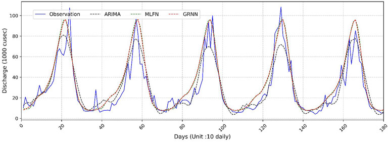
Figure 7. Comparison of predicted flow with the observed flows at Marala Headworks (year 2020–2024).

Figure 8

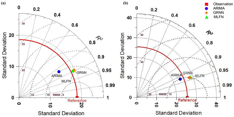
Figure 8. Statistical performance indicators of ARMIA, GRNN, and MLFN for (a) Mangla Dam and (b) Marala Headworks study locations.

4.3 Comparison of best fit models with IRSA forecast

A good forecasting model should demonstrate both robustness and reliability. In this study statistical performance indicators are used to choose the best model for each study location and selected model results are compared with the forecasted results of IRSA as shown in Figure 9, 10. IRSA forecasted the inflows using the probabilistic method and the lead time is 6 months as stated by various research studies (Charles et al., 2018; Umar, 2020). The Taylor diagram shown in Figure 11 summarizes forecasts of selected models with IRSA forecasted results in terms of statistical performance indicators. Figure 9 shows the comparison of GRNN forecast; IRSA forecast and observed inflows at Mangla Dam. Figure 11a depicted that the GRNN forecast shows the best correlation as compared with the IRSA probabilistic approach. In the case of Mangla Dam, the RMSE and R² factors for the GRNN forecast are improved by 15.52% and 5.70% as compared to the IRSA forecast. The detailed comparison of forecasted results of MLFN with IRSA drawn against the observed flows of Marala Headworks is shown in Figure 10. Figure 11B presents a Taylor diagram that summarizes the statistical performance of the selected MLFN model compared to the IRSA forecasted results. As depicted in Figure 11Bb the MLFN forecast exhibits the best correlation performance, surpassing the IRSA probabilistic approach. Specifically, for Marala Headworks, the MLFN forecast shows a 4.91% reduction in RMSE and 3.16% improvement in R² values, indicating a significant enhancement in predictive accuracy over the IRSA forecast.

Figure 9

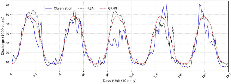
Figure 9. Comparison of predicted flows by GRNN Model and IRSA model with the observed flows at Mangla Dam (year 2020–2024).

Figure 10

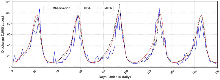
Figure 10. Comparison of predicted flows by MLFN Model and IRSA model with the observed flows at Marala Headworks (year 2020–2024).

Figure 11

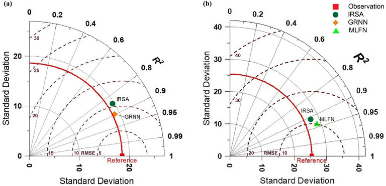
Figure 11. Comparative analysis of statistical performance indicators in case of (a) IRSA vs. GRNN for Mangla Dam and (b) IRSA vs. MLFN for Marala Headworks.

5 Discussions

Musarat et al. (2021) predicted the flows at Kabul River using the Automated ARIMA forecasting model. The flows in the Kabul River are prone to extreme floods and therefore it is of extreme importance for better predicting the flood water levels and assessment of flood discharge. The forecasted flows were assessed for their performance with the observed flows using statistical performance indicators ${\mathrm{R}}^2$, RMSE, MAE, and MAPE. Kerem (2005), studied the use of the Generalized Regression Neural Networks (GRNN) model for intermittent flow forecasting at three flow stations in the Thrace region of the European part of Turkey. The GRNN model was found superior to the traditional Feed-forward Back Propagation (FFBP) Model in flow forecasting based on selected performance criteria. It was found that GRNN does not forecast flows that are not physically conceivable. Rauf et al., 2018 did a comparative analysis of three AI models (Broyden-Fletcher-Goldfarb-Shannon, Conjugate Gradient, and Back Propagation Algorithm) with four regression models for streamflow forecasting in the Upper Indus Basin. The performance of these models was evaluated by using mean bias error, NSE, R^2, and correlation coefficient. Long-term streamflow forecasting has been made by using the best ANN Models.

Our study has evaluated inflow forecasting at Mangla Dam on the Jhelum River and Marala Headworks on the Chenab River by using a statical technique, i.e., ARIMA Model, and two Artificial Intelligence (AI) techniques, i.e., GRNN Model and MLFN Model. The prediction capabilities of the three selected models were assessed using statistical performance indicators ${\mathrm{R}}^2$, RMSE, and NSE, and based on these performance indicators and qualitative analysis results, the best-suited model for each study station was selected. Our study has revealed that AI models have outperformed the traditional statistical ARIMA model when it comes to better flow forecasting capability. The RMSE and R² in the case of ANN models are improved in the range of 3.30%–6.37% and 1.61%–6.62% respectively as compared to the ARIMA model. Our study has revealed that the GRNN model and MLFN model are the best-fit models for Mangla Dam on the Jhelum River and Marala Headworks on the Chenab River respectively. Charles et al. (2018) assessed the streamflow forecasting at Tarbela Dam on the Indus River and Mangla Dam on Jhelum using the Bayesian Joint Probability (BJP) statistical approach, using climate indices and antecedent flow conditions as predictors. In the case of Mangla Dam the author has compared the BJP forecasts with (1) Ensemble Streamflow Predictions (ESPs) from the snowmelt runoff model (SRM), (2) a Hybrid approach using BJP with SRM-ESP forecast. The BJP models were run with varying combinations of predictors considering the antecedent flow conditions.

For assessing the performance of flow prediction models the author has used skill scores based on the percentage reduction in the inter-quartile range (IQR) between the observed flow historical distribution and the forecasted flow distribution. The IQR is the measure of statistical dispersion which is the spread of the data and the skill scores were defined from http://www.bom.gov.au/water/ssf/faq.shtml. The performance of the BJP forecast in the case of Tarbela is poor as compared with forecasts at Mangla Dam and that can be attributed to the differences in flow generation mechanism. IRSA which is currently using a probabilistic method for the inflow forecasting at rim stations of the Indus River basin can also employ the BJP forecasting model. However, assessment of the results of the BJP model forecast would require informed and trained water professionals in Pakistan (Pagano and Hartmann, 2002; Ramos et al., 2013; Rayner et al., 2005; Sarah and Casey, 2015).

Our study has focused on the single input variable of flow discharge for inflow forecasting and has assessed the performance of inflow forecasting from the best suitable models at Mangla Dam on the Jhelum River and Marala Headworks on the Chenab River. In particular, when it comes to comparison with forecasted inflows of IRSA, the statistical indicators for ANN models (GRNN and MLFN) improved by an average of 4.43% in R² and 10.22% in RMSE, indicating a significant enhancement in predictive accuracy over the IRSA forecast. To enhance the inflow forecasting accuracy, IRSA may integrate the results from the current study into existing models.

6 Conclusion

This study investigates the inflow forecasting for Mangla Dam and Marala Headworks using the latest ANN models (GRNN and MLFN) and traditional statistical method (ARIMA) focusing on the forecasting challenges of IRSA using single input variables. Concerning the challenge of the single inflow variable, a comparative analysis was performed among forecasted inflows by GRNN, MLFN, ARIMA, and IRSA. The important conclusions are drawn as follows:

• Substantial improvement has been observed in the forecasting of inflows at both study locations using ANN Models compared to the statistical methods.

• The average RMSE and R² for ANN models obtained by GRNN and MLFN are improved by 4.84% and 4.15% compared to the ARIMA model. Moreover, qualitative analysis illustrated that ANN models are more capable of predicting low and peak flows with better accuracy.

• In particular, when it comes to comparison with forecasted inflows of IRSA, the statistical indicators for ANN models (GRNN and MLFN) improved by an average of 4.43% in R² and 10.22% in RMSE, indicating a significant enhancement in predictive accuracy over the IRSA forecast.

Despite achieving high prediction accuracy by using ANN models and outperforming the existing methods, future research may focus on exploring alternative integrated approaches. To enhance the inflow forecasting accuracy, IRSA may integrate the results from the current study into existing models. This study shows that ANN models have better accuracy in predicting inflows compared to traditional forecasting methods and compel water managers to adopt the latest techniques for sustainable water resource management.

Data availability statement

The original contributions presented in the study are included in the article/supplementary material, further inquiries can be directed to the corresponding author/s.

Author contributions

MK: Conceptualization, Formal Analysis, Methodology, Supervision, Writing – original draft. MS: Conceptualization, Formal Analysis, Methodology, Supervision, Writing – original draft. MZ: Conceptualization, Formal Analysis, Methodology, Supervision, Writing – original draft. MR: Conceptualization, Formal Analysis, Methodology, Supervision, Writing – original draft. MT: Conceptualization, Formal Analysis, Methodology, Supervision, Writing – original draft. SH: Data curation, Investigation, Project administration, Writing – review and editing. AO: Data curation, Investigation, Project administration, Writing – review and editing. AD: Data curation, Investigation, Project administration, Writing – review and editing. MM: Data curation, Investigation, Project administration, Writing – review and editing. AS: Investigation, Project administration, Supervision, Writing – original draft.

Funding

The author(s) declare that financial support was received for the research and/or publication of this article. This research was funded by Ongoing Research Funding program - Research Chairs (ORF-RC-2025-5504), King Saud University, Riyadh, Saudi Arabia.

Acknowledgments

The authors extend their appreciation to Ongoing Research Funding program - Research Chairs (ORF-RC-2025-5504), King Saud University, Riyadh, Saudi Arabia.

Conflict of interest

The authors declare that the research was conducted in the absence of any commercial or financial relationships that could be construed as a potential conflict of interest.

Generative AI statement

The authors declare that no Generative AI was used in the creation of this manuscript.

Publisher’s note

All claims expressed in this article are solely those of the authors and do not necessarily represent those of their affiliated organizations, or those of the publisher, the editors and the reviewers. Any product that may be evaluated in this article, or claim that may be made by its manufacturer, is not guaranteed or endorsed by the publisher.

References

Afan, H. A., Allawi, M. F., El-Shafie, A., Yaseen, Z. M., Ahmed, A. N., Malek, M. A., et al. (2020). Input attributes optimization using the feasibility of genetic nature inspired algorithm: application of river flow forecasting. Sci. Rep. 10 (1), 4684. doi:10.1038/s41598-020-61355-x

PubMed Abstract | CrossRef Full Text | Google Scholar

Agnihotri, A., Sahoo, A., and Diwakar, M. K. (2022). “Flood prediction using Hybrid ANFIS-ACO model: a case study bt - inventive computation and information technologies.” in Inventive Computation and Information Technologies. (Editors). S. Smys, V. E. Balas, and R. Palanisamy, 169–180. Singapore: Springer Nature.

CrossRef Full Text | Google Scholar

Ahmad, M. D., Cuddy, S. M., Podger, G. M., Yu, Y., and Perraud, J. M. (2023). “Water allocation planning in the Indus Basin Irrigation System in Pakistan: using scientific tools to build trust between stakeholders,” in 25th international congress on modelling and simulation. Darwin, NT, Australia. doi:10.36334/modsim.2023.ahmad252

CrossRef Full Text | Google Scholar

Ahmad, M.-D., Peña-Arancibia, J. L., Stewart, J. P., and Kirby, J. M. (2021). Water balance trends in irrigated canal commands and its implications for sustainable water management in Pakistan: evidence from 1981 to 2012. Agric. Water Manag. 245, 106648. doi:10.1016/j.agwat.2020.106648

CrossRef Full Text | Google Scholar

Ali, S., Cheema, M. J., Waqas, M. M., Waseem, M., Leta, M. K., Qamar, M. U., et al. (2021). Flood mitigation in the transboundary Chenab River basin: a basin-wise approach from flood forecasting to management. Remote Sens. 13 (19), 3916. doi:10.3390/rs13193916

CrossRef Full Text | Google Scholar

Araghinejad, S., Burn, D. H., and Karamouz, M. (2006). Long-lead probabilistic forecasting of streamflow using ocean-atmospheric and hydrological predictors. Water Resour. Res. 42 (3). doi:10.1029/2004WR003853

CrossRef Full Text | Google Scholar

Awchi, T. A. (2014). River discharges forecasting in northern Iraq using different ANN techniques. Water Resour. Manag. 28 (3), 801–814. doi:10.1007/s11269-014-0516-3

CrossRef Full Text | Google Scholar

Babur, M., Babel, M. S., Shrestha, S., Kawasaki, A., and Tripathi, N. K. (2016). Assessment of climate change impact on reservoir inflows using Multi climate-models under RCPs—the case of Mangla dam in Pakistan. Water 8 (Issue 9), 389. doi:10.3390/w8090389

CrossRef Full Text | Google Scholar

Box, G. E. P., Jenkins, G. M., Reinsel, G. C., and Ljung, G. M. (2015). Time series analysis: forecasting and control. John Wiley & Sons.

Google Scholar

Briscoe, J., and Qamar, U. (2006). Pakistan’s water economy: running dry. Available online at: https://hdl.handle.net/10986/11746.

Google Scholar

Charles, S. P., Wang, Q. J., Ahmad, M.-D., Hashmi, D., Schepen, A., Podger, G., et al. (2018). Seasonal streamflow forecasting in the upper Indus Basin of Pakistan: an assessment of methods. Hydrology Earth Syst. Sci. 22 (6), 3533–3549. doi:10.5194/hess-22-3533-2018

CrossRef Full Text | Google Scholar

Chen, A.-S., and Leung, M. T. (2005). Performance evaluation of neural network architectures: the case of predicting foreign exchange correlations. J. Forecast. 24 (6), 403–420. doi:10.1002/for.967

CrossRef Full Text | Google Scholar

Cheng, M., Fang, F., Kinouchi, T., Navon, I. M., and Pain, C. C. (2020). Long lead-time daily and monthly streamflow forecasting using machine learning methods. J. Hydrology 590, 125376. doi:10.1016/j.jhydrol.2020.125376

CrossRef Full Text | Google Scholar

Choi, C., Kim, J., Han, H., Han, D., and Kim, H. S. (2020). Development of water level prediction models using machine learning in wetlands: a case study of upo wetland in South Korea. Water 12 (Issue 1), 93. doi:10.3390/w12010093

CrossRef Full Text | Google Scholar

Chu, H., Wei, J., Wu, W., Jiang, Y., Chu, Q., and Meng, X. (2021). A classification-based deep belief networks model framework for daily streamflow forecasting. J. Hydrology 595, 125967. doi:10.1016/j.jhydrol.2021.125967

CrossRef Full Text | Google Scholar

Cui, F., Salih, S. Q., Choubin, B., Bhagat, S. K., Samui, P., and Yaseen, Z. M. (2020). Newly explored machine learning model for river flow time series forecasting at Mary River, Australia. Environ. Monit. Assess. 192 (12), 761. doi:10.1007/s10661-020-08724-1

PubMed Abstract | CrossRef Full Text | Google Scholar

Danandeh Mehr, A., Kahya, E., Şahin, A., and Nazemosadat, M. J. (2015). Successive-station monthly streamflow prediction using different artificial neural network algorithms. Int. J. Environ. Sci. Technol. 12 (7), 2191–2200. doi:10.1007/s13762-014-0613-0

CrossRef Full Text | Google Scholar

Hassan, M., and Hassan, I. (2021). Improving artificial neural network based streamflow forecasting models through data preprocessing. KSCE J. Civ. Eng. 25 (9), 3583–3595. doi:10.1007/s12205-021-1859-y

CrossRef Full Text | Google Scholar

Hassan, M., Shamim, M. A., Hashmi, H. N., Ashiq, S. Z., Ahmed, I., Pasha, G. A., et al. (2015). Predicting streamflows to a multipurpose reservoir using artificial neural networks and regression techniques. Earth Sci. Inf. 8 (2), 337–352. doi:10.1007/s12145-014-0161-7

CrossRef Full Text | Google Scholar

Ibrahim, K. S. M. H., Huang, Y. F., Ahmed, A. N., Koo, C. H., and El-Shafie, A. (2022). A review of the hybrid artificial intelligence and optimization modelling of hydrological streamflow forecasting. Alexandria Eng. J. 61 (1), 279–303. doi:10.1016/j.aej.2021.04.100

CrossRef Full Text | Google Scholar

Jajarmizadeh, M., Kakaei Lafdani, E., Harun, S., and Ahmadi, A. (2015). Application of SVM and SWAT models for monthly streamflow prediction, a case study in South of Iran. KSCE J. Civ. Eng. 19 (1), 345–357. doi:10.1007/s12205-014-0060-y

CrossRef Full Text | Google Scholar

Kerem, C. H. (2005). Application of generalized regression neural networks to intermittent flow forecasting and estimation. J. Hydrologic Eng. 10 (4), 336–341. doi:10.1061/(ASCE)1084-0699(2005)10:4(336)

CrossRef Full Text | Google Scholar

Khosravi, K., Panahi, M., Golkarian, A., Keesstra, S. D., Saco, P. M., Bui, D. T., et al. (2020). Convolutional neural network approach for spatial prediction of flood hazard at national scale of Iran. J. Hydrology 591, 125552. doi:10.1016/j.jhydrol.2020.125552

CrossRef Full Text | Google Scholar

Kisi, O., and Sanikhani, H. (2015). Prediction of long-term monthly precipitation using several soft computing methods without climatic data. Int. J. Climatol. 35 (14), 4139–4150. doi:10.1002/joc.4273

CrossRef Full Text | Google Scholar

Kopal, I., Labaj, I., Vršková, J., Harničárová, M., Valíček, J., Ondrušová, D., et al. (2022). A generalized regression neural network model for predicting the curing characteristics of carbon black-filled rubber blends. Polymers 14 (Issue 4), 653. doi:10.3390/polym14040653

PubMed Abstract | CrossRef Full Text | Google Scholar

Kovačević, M., Ivanišević, N., Dašić, T., and Marković, L. (2018). Application of artificial neural networks for hydrological modelling in karst. Građevinar 70 (01), 1–10. doi:10.14256/JCE.1594.2016

CrossRef Full Text | Google Scholar

Le, X.-H., Ho, H. V., Lee, G., and Jung, S. (2019). Application of long short-term memory (LSTM) neural network for flood forecasting. Water 11 (7), 1387. doi:10.3390/w11071387

CrossRef Full Text | Google Scholar

Li, K., Wan, D., Zhu, Y., Yao, C., Yu, Y., Si, C., et al. (2020). The applicability of ASCS_LSTM_ATT model for water level prediction in small- and medium-sized basins in China. J. Hydroinformatics 22 (6), 1693–1717. doi:10.2166/hydro.2020.043

CrossRef Full Text | Google Scholar

Musarat, M. A., Alaloul, W. S., Rabbani, M. B., Ali, M., Altaf, M., Fediuk, R., et al. (2021). Kabul River flow prediction using automated ARIMA forecasting: a machine learning approach. Sustainability 13 (19), 10720. doi:10.3390/su131910720

CrossRef Full Text | Google Scholar

Nguyen, A. D., Le Nguyen, P., Vu, V. H., Pham, Q. V., Nguyen, V. H., Nguyen, M. H., et al. (2022). Accurate discharge and water level forecasting using ensemble learning with genetic algorithm and singular spectrum analysis-based denoising. Sci. Rep. 12 (1), 19870. doi:10.1038/s41598-022-22057-8

PubMed Abstract | CrossRef Full Text | Google Scholar

Oyerinde, G. T., Fademi, I. O., and Denton, O. A. (2017). Modeling runoff with satellite-based rainfall estimates in the Niger basin. Cogent Food & Agric. 3 (1), 1363340. doi:10.1080/23311932.2017.1363340

CrossRef Full Text | Google Scholar

Pagano, T. C., Hartmann, H. C., and Sorooshian, S. (2002). Factors affecting seasonal forecast use in Arizona water management: a case study of the 1997-98 El Niño. Clim. Res. 21 (3), 259–269. doi:10.3354/cr021259

CrossRef Full Text | Google Scholar

Pan, M., Zhou, H., Cao, J., Liu, Y., Hao, J., Li, S., et al. (2020). Water level prediction model based on GRU and CNN. Ieee Access 8, 60090–60100. doi:10.1109/ACCESS.2020.2982433

CrossRef Full Text | Google Scholar

Pernot, P., and Savin, A. (2020). Probabilistic performance estimators for computational chemistry methods: systematic improvement probability and ranking probability matrix. II. Applications. J. Chem. Phys. 152 (16), 164109. doi:10.1063/5.0006204

PubMed Abstract | CrossRef Full Text | Google Scholar

Podger, G. M., Ahmad, M.-D., Yu, Y., Stewart, J. P., Shah, S. M., and Khero, Z. I. (2021). Development of the Indus River System model to evaluate reservoir sedimentation impacts on water security in Pakistan. Water 13 (Issue 7), 895. doi:10.3390/w13070895

CrossRef Full Text | Google Scholar

Ramos, M. H., Van Andel, S. J., and Pappenberger, F. (2013). Do probabilistic forecasts lead to better decisions? Hydrology Earth Syst. Sci. 17 (6), 2219–2232. doi:10.5194/hess-17-2219-2013

CrossRef Full Text | Google Scholar

Rasouli, K., Hsieh, W. W., and Cannon, A. J. (2012). Daily streamflow forecasting by machine learning methods with weather and climate inputs. J. Hydrology 414–415, 284–293. doi:10.1016/j.jhydrol.2011.10.039

CrossRef Full Text | Google Scholar

Rauf, A., and Ghumman, A. R. (2018). Impact assessment of rainfall-runoff simulations on the flow duration curve of the upper Indus River—a comparison of data-driven and hydrologic models. Water 10 (Issue 7), 876. doi:10.3390/w10070876

CrossRef Full Text | Google Scholar

Rauf, A. U., Ghumman, A. R., Ahmad, S., and Hashmi, H. N. (2018). Performance assessment of artificial neural networks and support vector regression models for stream flow predictions. Environ. Monit. Assess. 190 (12), 704. doi:10.1007/s10661-018-7012-9

PubMed Abstract | CrossRef Full Text | Google Scholar

Rayner, S., Lach, D., and Ingram, H. (2005). Weather forecasts are for wimps: why water resource managers do not use climate forecasts. Clim. Change 69 (2), 197–227. doi:10.1007/s10584-005-3148-z

CrossRef Full Text | Google Scholar

Remesan, R., Ahmadi, A., Shamim, M. A., and Han, D. (2010). Effect of data time interval on real-time flood forecasting. J. Hydroinformatics 12 (4), 396–407. doi:10.2166/hydro.2010.063

CrossRef Full Text | Google Scholar

Sarah, W. N. P. R., Casey, B., and Brown, C. (2015). Seasonal hydroclimatic forecasts as innovations and the challenges of adoption by water managers. J. Water Resour. Plan. Manag. 141 (5), 4014071. doi:10.1061/(ASCE)WR.1943-5452.0000466

CrossRef Full Text | Google Scholar

Shiri, J., Shamshirband, S., Kisi, O., Karimi, S., Bateni, S. M., Hosseini Nezhad, S. H., et al. (2016). Prediction of water-level in the Urmia Lake using the extreme learning machine approach. Water Resour. Manag. 30 (14), 5217–5229. doi:10.1007/s11269-016-1480-x

CrossRef Full Text | Google Scholar

Specht, D. F. (1991). A general regression neural network. IEEE Trans. Neural Netw. 2 (6), 568–576. doi:10.1109/72.97934

PubMed Abstract | CrossRef Full Text | Google Scholar

Tayfur, G., Moramarco, T., and Singh, V. P. (2007). Predicting and forecasting flow discharge at sites receiving significant lateral inflow. Hydrol. Process. 21 (14), 1848–1859. doi:10.1002/hyp.6320

CrossRef Full Text | Google Scholar

Umar, M. (2020). Application of regression in seasonal flow forecasting for Upper Indus Basin of Pakistan. Arabian J. Geosciences 13 (19), 1021. doi:10.1007/s12517-020-06029-8

CrossRef Full Text | Google Scholar

Uysal, G., ſorman, A. A., and ſensoy, A. (2016). Streamflow forecasting using different neural network models with satellite data for a snow dominated region in Turkey. Procedia Eng. 154, 1185–1192. doi:10.1016/j.proeng.2016.07.526

CrossRef Full Text | Google Scholar

Wang, J., Shi, P., Jiang, P., Hu, J., Qu, S., Chen, X., et al. (2017). Application of BP neural network algorithm in traditional hydrological model for flood forecasting. Water 9 (1), 48. doi:10.3390/w9010048

CrossRef Full Text | Google Scholar

Wang, W., Gelder, P. H. A. J. M. V., Vrijling, J. K., and Ma, J. (2006). Forecasting daily streamflow using hybrid ANN models. J. Hydrology 324 (1), 383–399. doi:10.1016/j.jhydrol.2005.09.032

CrossRef Full Text | Google Scholar

Yaseen, Z. M., Awadh, S. M., Sharafati, A., and Shahid, S. (2018). Complementary data-intelligence model for river flow simulation. J. Hydrology 567, 180–190. doi:10.1016/j.jhydrol.2018.10.020

CrossRef Full Text | Google Scholar

Yu, Z., Lei, G., Jiang, Z., and Liu, F. (2017). “ARIMA modelling and forecasting of water level in the middle reach of the Yangtze River,” in 2017 4th international conference on transportation information and safety (ICTIS), 172–177. doi:10.1109/ICTIS.2017.8047762

CrossRef Full Text | Google Scholar

Zhang, X., Peng, Y., Zhang, C., and Wang, B. (2015). Are hybrid models integrated with data preprocessing techniques suitable for monthly streamflow forecasting? Some experiment evidences. J. Hydrology 530, 137–152. doi:10.1016/j.jhydrol.2015.09.047

CrossRef Full Text | Google Scholar