Influence of water quality on satellite laser altimeter underwater measurement accuracy

With the growing demand for global water environment monitoring, satellite laser altimeters (SLA) have considerable advantages for underwater measurements. However, changes in suspended solids, turbidity, and other optical properties of water affect the propagation of SLA laser pulses in water. This can affect the accuracy and reliability of the measurements. This study analyzed the impact of water quality changes in the Oahu Island region of Hawaii on the accuracy of SLA un-derwater measurements based on ICESat-2, MODIS, Landsat-8, and in situ data. Underwater photons were obtained from ICESat-2 ATL03 data through an Adaptive Elevation Difference Threshold, combined with in situ data to calculate the potential altimetry deviation. Using the water quality data inverted from Landsat-8 as a reference, MODIS kd490 was implemented through random forest regression. The impact of water quality changes on the SLA accuracy was quantified by combining the altimetry bias and water quality data that matched the laser footprint. There is a positive correlation between water quality and photon water permeability. The more turbid the water quality, the smaller the proportion of photons that can penetrate the water surface. The maximum measurement deviation caused by multiple scattering of the water body could reach the meter level. Future underwater bathymetry corrections need to consider the impact of multiple scattering. The findings are of considerable importance for environmental protection, resource management, policy formulation, and SLA data processing.

1 Introduction

Accurate water depth measurement is of important in fields such as water resource management, infrastructure planning, and disaster prevention. It has been widely used in shoreline assessments, hydrological process analyses, sediment transport monitoring, and channel maintenance (Bergsma et al., 2021; Dong et al., 2019; Peña-Arancibia et al., 2024). Traditional water depth measurement methods such as field surveys and acoustic techniques, can be applied to various water environments and have real-time data processing capabilities. However, they have certain limitations in terms of cost, coverage, and time resolution (Costa et al., 2009; Kutser et al., 2020). Since the 1970s, the rapid development of satellite microwave remote sensing has enabled satellite altimetry technology to extract large-scale, high-precision, and high-frequency water depth information (Pereira, 2019; Parrish et al., 2019; Herzfeld et al., 2014).

Satellite altimetry technology can be divided into two categories: satellite radar altimetry (SRA) and satellite laser altimetry (SLA). The SRA obtains information such as sea level, gravity field, and depth using microwave radars such as radar altimeters. Its footprint is generally at the kilometer level, and the height measurement accuracy is at the decimeter level, such as TOPEX, Jason-1/2, and HY-2A/B/C/D (Ardalan et al., 2023; Wang J. et al., 2023; Xu et al., 2021b). Information like the vertical distribution and depth of ocean profiles is obtained via lidar and laser altimeters. The footprint size is usually at the meter level, and height measurement accuracy is at the centimeter level, such as ICESat-1/2, ZY3-02/03, and GF-7 (Abdalati et al., 2010; Li et al., 2020; Schutz et al., 2005; Tang et al., 2020a; Tang et al., 2020b). Compared with SRA, the advantages of SLR are its high vertical resolution, high measurement accuracy, and small footprint. It has considerable advantages for water depth measurements, especially in shallow water areas, and in assessing small-scale water bodies. However, various factors can affect the accuracy of final measurements (Caballero and Stumpf, 2023; Chen et al., 2022; Ma et al., 2019; Xu et al., 2024a). In terms of water depth measurements, influencing factors can be divided into the following three aspects (Table 1): the influence of the external environment, the data processing algorithm complexity, and the interaction between the water body and laser.

Table 1

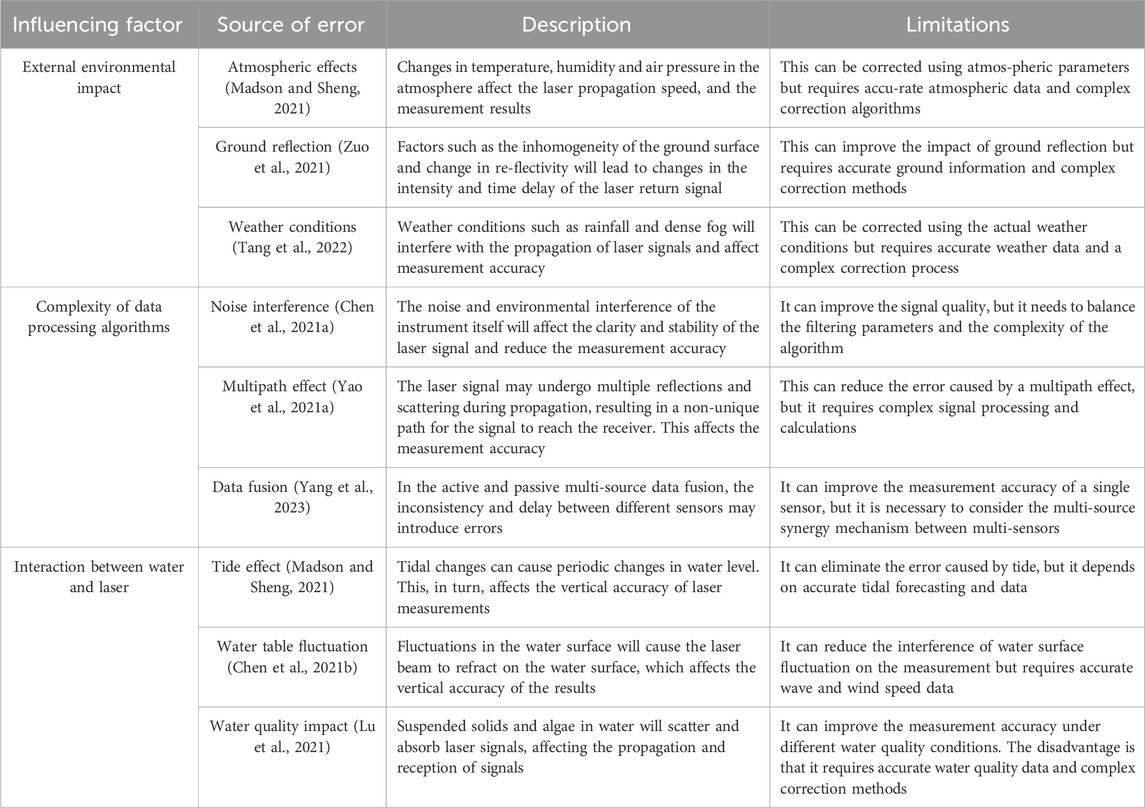
Table 1. Influencing factors of underwater measurement accuracy of satellite laser altimeter.

Laser pulse transmission from satellites to water bodies are affected by the external environment, such as cloud–aerosol layer obstruction, atmospheric multiple scattering, atmospheric refraction effects, and the surface slope. This directly reduces the laser penetration capability, signal quality, and flight conditions (Narin et al., 2024; Yao et al., 2021a; 2021b; Zuo et al., 2021). Studies have been conducted to correct the corresponding height measurement deviations using the corresponding models. If errors could not be eliminated, the data accuracy was controlled using quality control markers. Therefore, the influence of environmental factors can be appropriately resolved in engineering applications (Markus et al., 2017; Moudrý et al., 2022). From raw observation data to products that can be directly used by users, a series of data processing processes is required. This includes noise removal, active and passive sensor fusion, and other algorithms. Therefore, additional errors caused by the complexity of these algorithms must be considered. In severe cases, they may affect the data effectiveness (Cui et al., 2018; Xu et al., 2023). However, after nearly two decades of technological accumulation, satellite-ground multi-sensor fusion research has become relatively well developed and can achieve high-precision inversion of long-term and large-scale underwater characteristics (Leng et al., 2023; Yang et al., 2023). For underwater depth extraction using satellite altimetry technology, water quality parameters such as turbidity, suspended matter concentration, and water color may affect the detection of laser signals entering the water column and returning to the water surface. This interaction has a greater impact on the usability of the results (Hedley et al., 2021; Lu et al., 2023). In contrast with the problems faced in land areas, the distribution density of underwater signals varies with changes in water quality, seabed substrate, and seawater depth. The photon density varies significantly under different conditions. As the seabed topography changes, the degree of dispersion varies. Distinguishing signals from noise in complex situations is a key issue (Babbel et al., 2021).

The current ICESat-2 photon-denoising algorithm is mainly based on statistical distribution theory. This includes Adaptive Variable Ellipse Filtering Bathymetric Method (AVEBM), Density-Based Spatial Clustering of Applications with Noise (DBSCAN), Ordering Points To Identify the Clustering Structure (OPTICS), and an improvement algorithm to obtain signal photons using spatial clustering (Chen et al., 2021a). Currently, official products use histogram-based filtering algorithms. Although it is suitable for most situations, its accuracy is poor in areas with complex terrain (Neumann et al., 2021). AVEBM determines filtering parameters using the photon density distribution in different water environments and water depths to accurately detect signals on the water surface and underwater (Chen et al., 2021b; Ni et al., 2024; Xu et al., 2024b; Xu et al., 2021a; Yao et al., 2025). DBSCAN is the most widely used denoising model. This model proposes an adaptive density segmentation model that can detect vertical hierarchical structures such as the ground, vegetation canopy, and water surface in the data (Schubert et al., 2017; Xu et al., 2022b). The DBSCAN effect depends on the preset parameters. However, owing to the substantial amount of underwater background noise, selecting different input parameter values leads to significantly different clustering results and regional mobility crosses (Lao et al., 2021; Xu et al., 2022b). In contrast with the DBSCAN algorithm, although the OPTICS algorithm does not explicitly create clusters, it still relies on key parameters such as the minimum number of neighborhood points, Minpts, and the clustering radius Eps (Ankerst et al., 1999). No matter which algorithm is used, water quality directly affects the distribution of underwater photons. This directly affects the measurable limit underwater depth, and also affects the reliability and availability of data. Changes in water quality may originate from natural processes, such as sediment transport and algal blooms, or human activities, including pollution and changes in water bodies (Zheng et al., 2023). Therefore, understanding the impact of water quality changes on the underwater measurement accuracy of SLA is crucial for the application of SLA technology for inversion of underwater characteristics.

The ICESat-2 satellite photon point cloud has a strong water projection capability but is limited by factors such as spot size, underwater sediment, and water quality. As photons enter the water, water quality differences at different height levels along the transmission path cause multiple scattering and reflections. The energy gradient attenuation affects the ultimate detection distance. However, the complexity of multiple scattering introduces problems in the final result. This can result in inestimable measurement errors. Therefore, two problems must be solved urgently in the field of underwater detection: 1) Under what water quality threshold can errors be corrected? 2) Under what water quality threshold can the error no longer be corrected but can be corrected through quality control identification to quantify its impact? This study combined ICESat-2, MODIS, Landsat-8, and in situ data to analyze the impact of water quality changes in the Oahu Island area on the SLA underwater measurement accuracy. The study aimed to provide guidance for satellite laser altimetry data processing, quality control, and error.

2 Materials and methods

2.1 Regional overview

To further illustrate the impact of water quality changes on the underwater measurement accuracy of the satellite laser altimeter, the coastal zone of Oahu was selected as the experimental area, as shown in Figure 1a. Oahu Island is located in the middle of the Pacific Ocean and is the third largest Hawaiian island of the United States. It has a high level of coastline diversity. This area’s meteorological and seasonal changes can cause various changes in water quality, which align with the current study. The red area in Figure 1a represents the survey area. A buffer zone with a radius of 100 m was established using measured data. The parameters of the measured data are described in detail below. As shown in Figure 1b, for the ICESat-2 532 nm channel, the laser incurs incidence, refraction, and scattering on the atmosphere–ocean transmission path. Vertical incidence does not cause additional errors, and the refraction error is obtained. This has been corrected, but scattering errors remain a problem. Suspended particles such as silt, sediment, and phytoplankton, biological debris, and dissolved substances in water may undergo multiple Rayleigh scattering with photons. This can result in an inestimable delay distance, ultimately biasing the water depth measurement, which may be relatively large, or attenuated to the noise distribution level (Figure 1c). Affected by multiple atmospheric–water scattering, these signals are mixed with other photon point clouds and have a greater impact on the overall accuracy and user use. Quantifying this impact was one of the objectives of the present study.

Figure 1

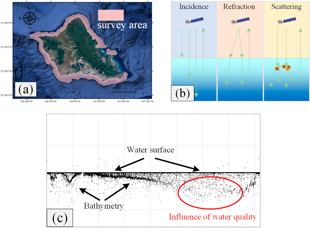
Figure 1. Overview of experimental area and principles. (a) Survey area. (b) Laser transmission path in water. (c) ATL03 typical underwater signal distribution.

2.2 Experimental data

This study mainly involved the water depth and quality data of the Oahu coastal area from 2018.09 to 2022.09 in Table 2. We used in situ data as reference water depth data and established a buffer zone as the research scope of this study. The in-situ data were point cloud data obtained through airborne LIDAR (SHOALS 3000) in 2013. Its expected water depth measurement accuracy could reach approximately 0.2 m (Xu et al., 2022a). Although the in-situ data were obtained in 2013, the underwater terrain did not change significantly. Therefore, we still used it as a reference for the true value of water depth. We used the ICESat-2 L2A global geolocation photonic product (ATL03) as the original measurement data. This contains the position information of all the data received by the satellite receiver, including orbital distance, elevation angle, longitude and latitude, and photon flight time, as shown in Section 3.1. Only by processing the algorithm can we obtain accurate water depth data, and its expected accuracy is approximately 0.5 m (Neumann et al., 2021). To obtain the changes in water quality, we quoted the diffuse reflection attenuation coefficient (Kd490) in the MODIS 3 L OceanColor product as a reference. Kd490 is the absorption coefficient of the water color index at 490 nm in water body. It is used to assess the concentration of suspended particulate matter in the water, reflecting the transparency and water quality of the water body. Since it falls between the green and infrared spectral bands and is close to the 532-nm wavelength of laser light, this study utilizes Kd490 to quantify the water quality and evaluate its impact on laser scattering(Lu et al., 2016). However, there was a substantial difference between its spatial resolution and the laser footprint size. Therefore, we used the algorithm in Section 3.2. Multiple water quality data such as sage depth inverted from Landsat-8 were used as references to achieve downscaling through random forest regression (Tilstone et al., 2021).

Table 2

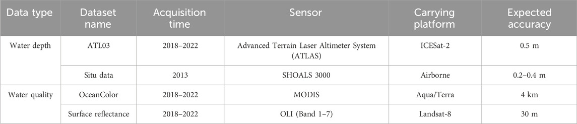
Table 2. Datasets covered in this article.

3 Experimental principles

The overall technical process is shown in Figure 2 and includes three main parts: data processing, and data analysis. The photon coordinates of different levels of the water body are obtained from the ICESat-2 ATL03 product through the AEDTA algorithm. Three types of reference water quality raster data were inverted through Landsat-8. The classified photon coordinates were corrected for refraction, and for use as the water quality reference. The data was obtained as a MTSI raster, and all the data were geo-referenced and resampled uniformly to ensure that the size of all the random forest data to be input was completely consistent. The downscaled Kd490, underwater altimetry error, and water permeability were combined as rate data. The impact of water quality changes on satellite laser altimetry data was analyzed from a spatial and trend perspective, and an empirical correction model was established.

Figure 2

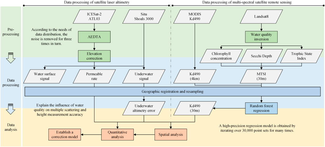
Figure 2. Overall process of the algorithm in this study.

3.1 Adaptive elevation difference threshold

ICESat-2 was launched in September 2018 and emits three pairs of laser micro pulses at a frequency of 10 kHz using an Advanced Terrain Laser Altimeter System (ATLAS). The 532 nm wavelength makes it water-permeable but is limited by the reflectivity of seawater to return photons (Wen et al., 2024a). Meanwhile, the 532 nm green light in sunlight is also captured by the satellite’s receiving field of view. Therefore, a substantial amount of background noise was mixed with the effective water depth signal in the acquired ATL03 data. The signal also includes the influence of terrain, clouds, and underwater obstructions. Therefore, a denoising algorithm was required to extract the water depth information (Wen et al., 2024b). In this study, the Adaptive Elevation Difference Threshold (AEDTA) was used as the denoising model. The specific process is as follows (Wang B. et al., 2023).

3.1.1 Surface, water, and underwater photon point cloud recognition model

Given that there are significant differences in the distribution of photons on the water surface, above water, and underwater, and because photons undergo refraction effects when they are transmitted in water, it is necessary to classify the original data hierarchically and denoize each layer of photons separately to obtain an effective signal. The accurate identification of these three photon layers is a key issue for water depth surveying and mapping. Given that only a few photons penetrate the water surface and most remain there, the water surface elevation can be determined based on the elevation value that appears most frequently in the elevation histogram. The Gaussian fitting model was used to determine the dense elevation distribution area along the track direction, that is, the photon elevation corresponding to the maximum amplitude. This is defined in Equations 1, 2:

$f\left(h\right)=A\times \mathit{exp}\left\{-\frac{{\left(h-\mu \left(h\right)\right)}^2}{2\times {\sigma \left(h\right)}^2}\right\}(1)$

$\left\{\begin{array}{l}h>\mu \left(h\right)+3\times \sigma \left(h\right),Photonsofabovewater\\ \mu \left(h\right)-3\times \sigma \left(h\right)<h<\mu \left(h\right)+3\times \sigma \left(h\right),Photonsofwatersurface\\ h<\mu \left(h\right)-3\times \sigma \left(h\right),Photonsofunderwater\end{array}\right.(2)$

where f represents the Gaussian fitting model, h represents the height of the photon along the track direction, μ(h) represents the horizontal position of the fitted Gaussian peak position, σ(h) represents the width of the fitted Gaussian peak, and A represents the fitting. The maximum amplitude of the Gaussian model is the photon elevation of the water surface. After determining the photons on the water surface, a hierarchical classification of the photons was obtained based on the probability distribution rules of the ideal Gaussian model.

3.1.2 Underwater photon three denoising model

Underwater terrain in shallow sea areas is generally gentle and continuous, and the maximum depth measurement capability of lasers is often between 20 and 50 m. Within this range, it is assumed that the difference in elevation between adjacent photons does not exceed a certain threshold. If the threshold is satisfied, then the constraints enable rapid underwater signal recognition. Taking the elevation difference as the vertical axis and the starting coordinate of the photon in the long-track direction as the horizontal axis, we found that its spatial distribution is similar to that of the exponential decay model. Therefore, we used Equations 3, 4 to rapidly calculate this threshold:

$h_{diff}=\left|h_{i+1}-h_i\right|(3)$

$f_{diff}\left(h_{diff}\right)=a\times \mathit{exp}\left\{-b\times hist\left(h_{diff}\right)\right\}+c(4)$

where h_i represents the height of the ith photon, h_diff represents the absolute value of the height difference between adjacent photons, f_diff(h_diff) represents the exponential decay model, and hist(h_diff) represents the abscissa of the statistical histogram. This is the starting point of adjacent photons along the track. In terms of coordinates, a represents the amplitude of the attenuation model, b represents the attenuation rate of the attenuation model, and c represents the constant term of the attenuation model, respectively. The spatial distribution of the elevational differences at each location can be obtained through this attenuation model. The threshold was determined using Equation 5, where hthr represents the threshold.

${f_{diff}\left(h_{diff}\right)-c<1\times {10}^{-3},h}_{thr}=h_i(5)$

This was used as the basis for performing the three denoising operations. The three denoising methods were required to make accurate estimates of the different photon distributions in complex environments. In the first denoising step, all underwater photons were targeted. When the elevation difference was greater than a threshold, the two adjacent photons were marked as noise. By contrast, the two photons were marked as signals. For the second denoising, the photons marked as noise in the first denoising result were used as targets, and the threshold was redetermined for denoising. For the third denoising, the photons marked as noise in the second denoising result were used as targets, and the threshold was determined again for denoising. The photons marked as signals after the three denoising cycles were the final outputs of the underwater signals. The advantage of this model is that it does not require manual determination of parameters and adapts to the characteristics of ICESat-2 ATL03 data to derive thresholds.

3.1.3 Water depth estimation model

As the water depth increases, the photon transmission path undergoes refraction effects, causing measurement deviations. A water depth of 30 m causes an elevation measurement offset of approximately 9 cm (Parrish et al., 2019). Therefore, for shallow water depth detection, the following empirical model, as shown in Equation 6, was used to correct the refraction error (Parrish et al., 2019):

$h_{cor}=h_{ph}+0.25416\times \left(ssh-h_{ph}\right)(6)$

where h_cor represents the corrected photon water depth, ssh represents the water surface height, and h_ph represents the underwater signal height after denoising.

3.2 Principle of the water quality inversion and downscaling algorithm

The spatial and temporal resolution of the MODIS Level 3 ocean water color product is 4 km on a daily scale. This makes it difficult to directly match the size of the satellite laser footprint. Therefore, in this study, we used the 30 m Mean Trophic State Index (MTSI) retrieved from Landsat-8 as water quality reference data. These data were fed into the random forest model to achieve spatial resolution downscaling. Water quality parameter inversion primarily uses the radiation energy received by the sensor to analyze the water quality parameters. In this study, to avoid interference from environmental factors on water quality inversion, we selected chlorophyll a concentration, sage depth, and the nutritional status index for the MTSI inversion. Three basic performance indicators were selected. The specific descriptions are as follows.

3.2.1 Water quality inversion algorithm

Chlorophyll concentration a (Chla) captures solar energy and converts it into biomass for plants and algae. Its concentration is an important parameter in evaluating the ecological health and nutritional status of water bodies. High chlorophyll a concentrations usually indicate that there are too many nutrients in the water body and that the water body is eutrophic. Low chlorophyll a concentrations indicate a lack of adequate nutrients in water to support a healthy ecosystem. The chlorophyll a concentration in water bodies differs. The corresponding spectral information from the remote sensing images also differs. Generally, the spectral characteristics of water bodies containing chlorophyll a have the highest values in the near-infrared band. Therefore, the following inversion model, as shown in Equation 7, was constructed:

$Chla=\left(0.06\times B_4+0.00638\right)/10000(7)$

where Chla represents the chlorophyll a concentration in μg/L, and B4 represents the characteristic band in the near-infrared band range of the Landsat-8 image.

Secchi depth (SD) reflects the transparency of water and is an important parameter that describes the optical properties and quality of water. Suspended substances, particles, or sediments in the water body scatter and absorb light, reducing the transparency of the water body. This results in a reduction in the SD. Multispectral remote sensing inversion technology analyses the relationship between different wavebands to achieve broader and more detailed water transparency monitoring and SD estimation, compensating for the lack of local data caused by the inability of ships to reach the traditional Secchi Pan method. In Equation 8:

$SD=0.1777\times {10}^{1.4856\times \mathit{ln}\left(\frac{B_2}{B_4}\right)+0.2734}+1.0813(8)$

SD represents the Secchi Depth (m) and B₂ and B₄ represent the green and near-infrared band of the Landsat8 image, respectively.

The Trophic State Index (TSI) was originally proposed by Carlson (1977). He determined the TSI of lake water based on the chlorophyll a (Chla) content. The calculation method, as shown in Equation 9, is as follows:

$TSI=10\times \left[6-\left(2.04-0.68\ln \left(Chla\right)\right)/\ln 2\right](9)$

where TSI is the Carlson nutritional status index and Chla is the chlorophyll a concentration in the water (µg·L⁻¹).

The MTSI is used to describe the trophic status of a specific lake’s waters. The calculation of MTSI value mainly uses the following formula, as shown in Equation 10, which is a multiparameter evaluation standard. This method eliminates the dependence on a single factor.

$MTSI=\frac{\left[CHL+SD+TSI\right]}{3}(10)$

3.2.2 Water quality super-resolution reconstruction algorithm

Random forest regression (RFR), a powerful machine learning method, has shown broad potential in the field of super-resolution reconstruction of water quality data owing to its nonlinear modeling capabilities and adaptability to various data. In terms of application prospects, super-resolution reconstruction, also known as downscaling sampling, refers to the process of converting low-resolution data into high-resolution data and is crucial for improving the accuracy and efficiency of water quality monitoring (Wang et al., 2021).

In this study, we constructed multiple decision trees using RFR, inferred the prediction results of the sample set on each independent individual tree, and used the verification set as the standard to quantify the training effect. The original data in the sample and validation sets refer to the MTSI data obtained from Landsat-8. The corresponding labels refer to MODIS KD490 water quality data. 4 km resolution MODIS was expanded into the same matrix shape as a 30 m Landsat-8. Using the results of georeferencing and matrix matching, the point set corresponding to both was constructed and divided 80% into the sample set and 20% into the validation set. The sample set was then sent to the RFR for iterative training. In this process, we used the following parameters as evaluation indices, as shown in Equation 11:

$RSR=\frac{RMSE}{STDEV}=\frac{\sqrt{{\sum }_{\mathrm{i}=1}^{\mathrm{n}}{\left({\mathrm{y}}_{\text{predi}}-{\mathrm{y}}_{\text{obsi}}\right)}^2}}{\sqrt{{\sum }_{\mathrm{i}=1}^{\mathrm{n}}{\left({\mathrm{y}}_{\text{obsi}}-\overline{{\mathrm{y}}_{\text{obsi}}}\right)}^2}}(11)$

where RSR is the root mean square error (RMSE)-observations standard deviation ratio (RSR). RMSE refers to the root mean square error between the prediction result and the observation results. STDEV refers to the standard deviation of the observation data, and n refers to the number of data. y_predi refers to the prediction result, which is the underwater elevation measurement value; y_obsi is the observation result, which is the true value of the underwater elevation; and $\overline{y_{obsi}}$ is the mean value of the observation result. In this study, we used the Scikit-learn package to initialize the RFR and save the model parameters (Pedregosa et al., 2012).

4 Results

4.1 Influence of water quality on satellite laser measurement accuracy

Figure 3a shows the distribution of laser points and water quality data in the shoal area of Oahu. There were 125 tracks of ICESat-2 laser data from this area, comprising a total of 376,050 laser photons. These photons include noise and signal photons, and the signal photons did not necessarily return to values underwater. The water quality data visualized in Figure 3a were averaged from the daily scale Kd490 data and obtained using random forest analysis. The Diffuse Attenuation Coefficient (Kd490) represents the absorption and scattering ability of the water body in the 490 nm channel. It is often used in water quality and oceanography to evaluate the optical properties of water bodies, particularly for studying the content and distribution of phytoplankton in water. Larger values indicate higher turbidity and poorer potential water quality.

Figure 3

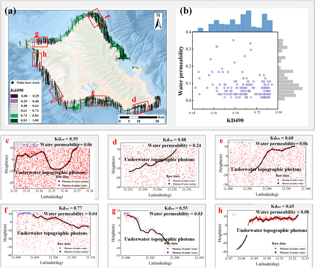
Figure 3. (a) Laser point and water quality data distribution of shoals in the Oahu area. (b) correlation between water quality and water permeability; (c–f) the sounding result during the day; (g, h) the sounding results at night.

Overall, the water quality fluctuations in the Oahu shoals vary from 0 to 1 and are relatively uniform. The north and southwest areas had the worst and best water quality, respectively. The further away from the shore, the smaller the value. To gain an in-depth understanding of the impact of water quality changes on satellite laser water permeability and height measurement accuracy, six areas with different water quality gradients were selected for further analysis, as shown in red framed areas c–h in Figure 3a. Different gradient ranges were formed by the natural discontinuities. Figure 3a shows the photon spatial distribution map corresponding to the laser point trajectory. Figures 3c–f is the sounding result during the day, and Figures 3g,h are the sounding results at night. In this figure, the horizontal axis represents the photon dimensions along the track. The vertical axis is the height along the track, blue represents the water surface photon recognized by AEDTA, and red represents the underwater photon recognized by AEDTA. Kd490 is the average value of the regional along-track data. Water permeability is calculated as the proportion of the number of underwater photons to the overall effective signal. Water permeability is an evaluation of the ability of a satellite laser altimeter to penetrate and obtain effective signals under different water quality conditions.

The results show that there was a correlation between water quality and water permeability, as shown in Figure 3b. Poor water quality often implies a low permeability. Among them, when Kd490 is in the range of 0.57–0.72, the water permeability was the lowest. This may be because of the presence of more dissolved organic matter and suspended particles in the water body. These prevent light from fully penetrating the water body, thus affecting the laser transmittance. Higher water permeability usually means that the water body has a stronger ability to transmit light. This is more likely to cause the photon signal to penetrate deeper water layers, thus affecting the sounding results. Compared to areas of high water quality, there may be more suspended particulate matter in water bodies in areas of low water quality. Particulate matter can cause scattering, absorption, or reflection of laser signals, resulting in the generation of noise points and loss of photons in the water. The signal was more dispersed, thus interfering with the bathymetry results. This trend is evident in Figures 3c–h. When the track passes through water during the day Figures 3c–f, the lower the Kd490 value, the higher the water permeability, and the photons can better display the underwater topography, thereby obtaining more accurate bathymetry results. Likewise, the night Figures 3g–h exhibited similar characteristics.

For a photon-counting system satellite laser altimeter, the background noise acquired during the day and night may differ significantly. To obtain a more universal conclusion based on Figure 3, water quality and water permeability were analyzed on a continuous spatial scale. The correlation between water quality and water permeability is shown in Figure 4. The diffuse reflection coefficient, Kd490, represents the ability of the water body to weaken the laser. Its value range is 0–1. When it was 1, the laser pulse attenuated almost completely.

Figure 4

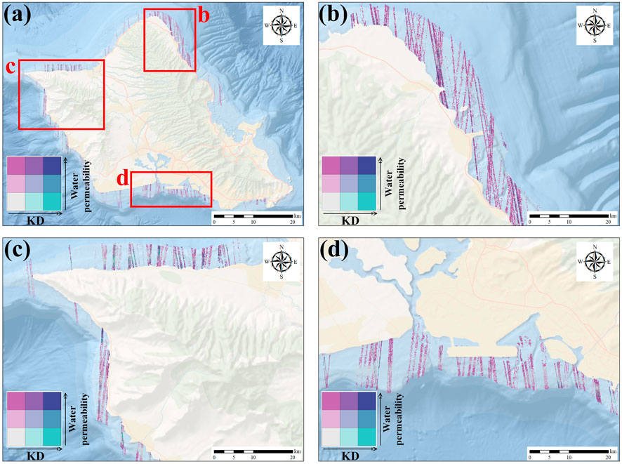
Figure 4. Spatial correlation between water quality and water permeability. (a) Overall spatial distribution; distinct areas in Oahu: (b) the upper area, (c) the central area, (d) the lower area.

Figure 4a shows the spatial distribution of the dual variable correlation between water quality and water permeability. According to the numerical change range of the two variables in the study area, each variable was reclassified into three categories (Kd490: [0.281, 0.335)/(0.335, 0.359)/(0.359, 1)]; water permeability: [0.018, 0.092)/(0.092, 0.259)/(0.259, 1)]).

Overall, Oahu’s regional water quality and permeability showed an interactive and mutually influential relationship. Water permeability refers to the ability of soil or other media to pass through its surface to the surface or groundwater below. We observed distinct areas in Oahu. Figure 4b in the upper area and Figure 4d in the lower area showed that areas with lower water quality but higher water permeability could be observed. This may be due to high water permeability, which makes it easier for pollutants in the water to penetrate groundwater or deep soil, causing groundwater contamination and worsening water quality. Excessive water permeability may increase surface runoff, exposing the water body to pollutants and thereby reducing water quality. In contrast, the central area in Figure 4c shows higher water quality and water permeability. This is because the water permeability level directly affects the residence time and flow rate of water in the soil or medium. When soil water permeability is high, water penetrates deeper into the soil more easily. This helps improve water quality because microorganisms and soil particles in the soil can filter and adsorb pollutants in the water.

4.2 Impact of long-term water quality on the underwater measurement accuracy of satellite laser altimetry

Figure 5 shows the measurement error of the intersecting tracks in different waters. The orbit error in the figure refers to the sounding difference of the two intersecting tracks in the same area. The result shows there are certain differences in the photon-sounding results in the intersecting parts of the tracks. As the depth increases, this difference gradually increases. In Figure 5, we selected three areas with similar water quality distributions to reflect the differences in the bathymetry results, Where the orange box area is the crossing position of the two laser orbits. As shown in Figures 5a,b, the two tracks intersected near the water surface. The differences in the depths of the two tracks were small at 0.144 and 0.314 m, respectively. In Figure 5, we selected three areas with similar water quality distributions to reflect the differences in the bathymetry results. However, as the water depth increased (Figure 5c), the water characteristics became more complex, causing the laser signal to become more affected during propagation. This increased the difference in the bathymetry results, reaching 0.507 m. The accuracy of water body bathymetry was correlated with the season and strength of the photon signal. Figures 5a,c show the strong and weak orbits, respectively. Compared with weak orbits, the photon signals received in strong orbits were stronger and richer, which makes them more accurate. Water depth measurements in Figure 5b show the photon track bathymetry results in different seasons (December and July). Compared to summer, the photon signal in water was stronger in winter, resulting in differences in the water depth measurements.

Figure 5

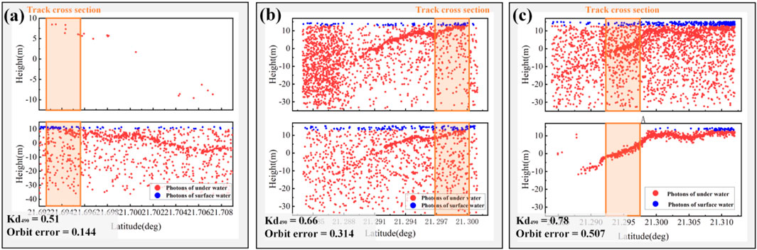
Figure 5. Spatial distribution of laser points between cross rails. (a, b) the two tracks intersecting near the water surface, (c) Intersecting in the deep water.

To further analyze the difference in underwater ranging accuracy between strong and weak laser beams, three cases were selected, and the bathymetric results of the simultaneously observed strong and weak laser beams were analyzed. The results are shown in Figure 5. There were differences in the water depth measurement results of different strong and weak beams. Compared with real bathymetry results, strong beams usually provide more accurate bathymetry. From the perspective of the photon signal reflection, strong beams exhibit stronger photon signals during underwater measurements. This may mean that the strong beams can penetrate deeper into the water body. The propagation path of the photon signal in the water body is stronger, thus providing a stronger reflection signal. From the perspective of bathymetry performance, the signal intensity of the strong beam was greater. Therefore, the bathymetry results were more accurate than those of weak beams. In Figure 6, we compared the preliminary depth-sounding values and real values of the strong and weak beams in different areas. In Figure 6, the mean Kd490 values in the region shown in Figures 6a,b,c are 0.25,0.39, and 0.59, respectively and the corresponding average track errors were 1.13 m, 1.36 m, and 2.93 m, showing a positive correlation. In different areas at three different times, the maximum errors between the strong beam and the true value were 6.375 m, 7.614 m, and 2.931 m respectively. Meanwhile, the maximum errors between the weak beam and the true value were 5.243 m, 8.976 m, and 10.231 m, respectively. This shows that strong beams perform better in terms of depth measurement accuracy than weak beams. However, because a strong beam is more sensitive to suspended particles in the water when the water quality is poor and the Kd490 is greater than 0.5. There may be more noise photons in the water, which will affect the accuracy of the water depth measurement.

Figure 6

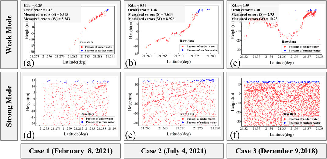
Figure 6. Analysis of the difference in underwater ranging accuracy between strong and weak laser beams. (a–c) weak laser beams, (d–f) strong laser beams.

4.3 Underwater scattering error correction based on the empirical model

The fitting relationship between the water quality and underwater elevation measurement error is shown in Figure 7. The linear fitting slope of the two is 6.18 and the intercept is 0.85. A positive correlation was observed between the two with a correlation coefficient of 0.72. The deviation (Bias) between water quality and underwater altimetry error was −2.56, indicating that on average, the underwater altimetry error is slightly lower than that of the water quality data. This may be due to systematic deviations during the data collection process, resulting in errors in the altimetry data. The Mean Absolute Percentage Error (MAPE) were 96.85%. This indicated that there were certain differences between the underwater altimetry data and water quality data. The variability in the altimetry data affected the water quality data to a certain extent. This variability was not highly interpretable and may be related to the presence of noisy photons. As the underwater height measurement error and Kd490 decrease, the scatter point distribution gradually becomes denser, indicating that when the water quality is high, the underwater height measurement error is lower and the measurement accuracy is higher. When the water quality is poor, the laser transmittance is higher. If the value is low, the photon noise points increase and the measurement accuracy will also decrease. When Kd490 was less than 0.14 and the height measurement error was less than 0.17, the concentration of scattered points in the two-dimensional space was the highest.

Figure 7

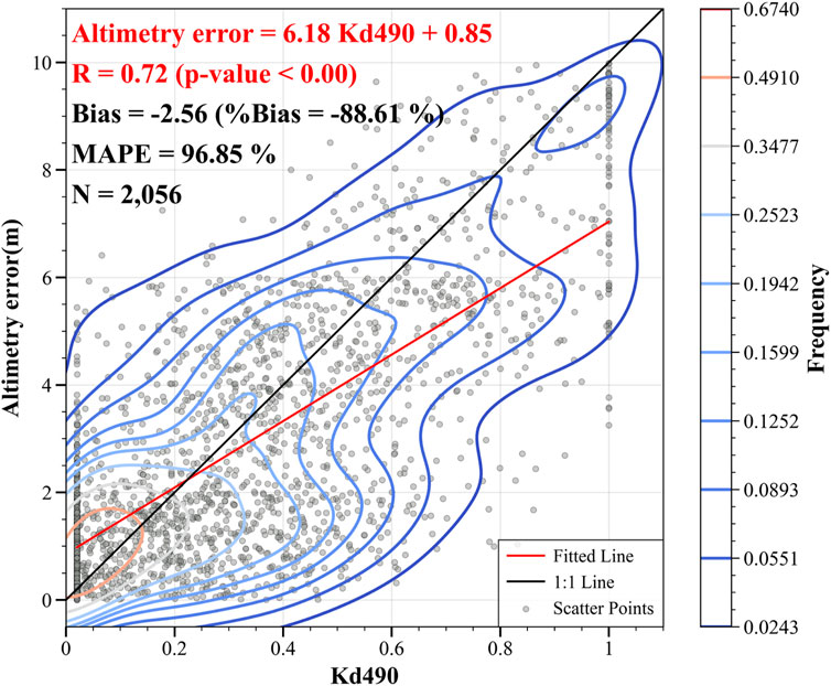
Figure 7. Empirical fitting model between water quality and underwater measurement errors.

To eliminate errors caused by the combined effects of sound speed, water temperature, and salinity, we performed denoising correction processing on the underwater ranging errors to improve the accuracy and credibility of the data. A histogram of the underwater ranging errors before and after the correction is shown in Figure 8. Before correction, we observed that 50% of the data error range was distributed between 0 and 2. Meanwhile, the remaining 50% of the data error range was distributed between 2 and 7, and some of the data exceeded seven. However, after correction, the distribution of the data changed significantly. Seventy-five percent of the data error range was between 0 and 4, while the remaining 25% of the data error range was between 4 and 7. However, there were still a few data errors. After correction, the proportion of data with an error range between 2 and 4 increased significantly from 20% before correction to 40%. The maximum error value before correction could reach 10, while the maximum error value after correction dropped to seven. This showed that the denoising correction processing of underwater ranging errors can effectively reduce the error level, improve the quality and accuracy of data, and improve the readability and interpretability of processed data.

Figure 8

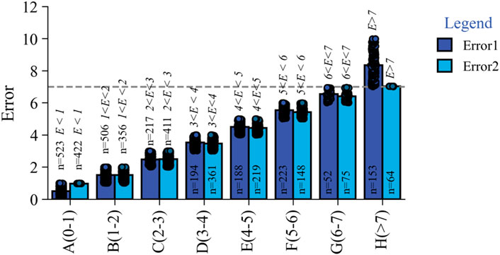
Figure 8. Comparison of statistical histograms of underwater ranging errors before and after correction.

To visually display the differences before and after underwater measurement height correction, three areas with large differences in water quality were selected for display. The results are shown in Figure 9. Figure 9b,c show two areas with relatively similar locations. The results show that the heights along the track in Figures 9a–c decreased to varying degrees after correction compared with before correction, by 2.40 m, 3.32 m, and 6.10 m, respectively. There is a certain correlation between the results before and after photon-sounding correction and the water quality. When Kd490 is larger, the difference in height along the track before and after correction is larger. This is because, when the water quality is poor, impurities, dissolved substances, or turbidity in the water are high, resulting in a murky water body. Increased scattering of laser light leads to increased uncertainty in elevation measurements. For different seasons (Figures 9b,c), there were large differences in height along the track before and after correction in winter. This may be because Oahu Island experiences more rainfall and lower temperatures in winter than in summer, causing changes in the concentrations of suspended sediment and particulate matter in the water. This affects the water quality, thereby affecting the laser height measurements.

Figure 9

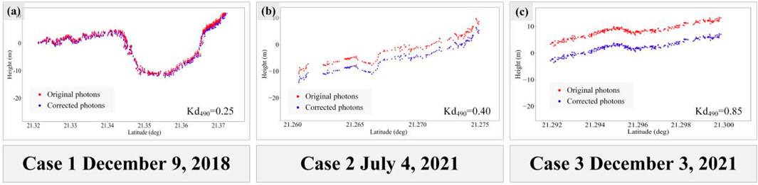
Figure 9. Display of the results of correcting the front and rear track heights. (a) Minor differences, (b, c) Significant differences.

5 Discussion

5.1 Limitations of the model proposed in this manuscript

The existing research on the impact of water quality changes on the accuracy of satellite laser height measurements is not completely clear. This study establishes an empirical model based on water quality and LIDAR verification data for the Oahu Island area to quantify this impact. However, three potential issues need to be addressed. Firstly, the weak data generalization ability of the empirical model was constructed using the Oahu Island area and may only represent a this specific geographic location or water condition. The accuracy and generalizability of the model may be affected if it is applied to different regions or environmental conditions. For example, a model built in an estuarine region may not be applicable to the open ocean because the water quality characteristics of the two environments differ significantly. Secondly, dynamic changes in time and space of aquatic environments are dynamically changing, including seasonal changes, weather effects, and human factors. This may lead to rapid changes in water quality. Empirical models are often built using historical data and may not effectively capture short- and long-term environmental changes. Therefore, models may need to be updated regularly to maintain their accuracy in changing environments. Furthermore, terrain changes may render past data inadequate for meeting real-time satellite measurement accuracy assessment needs. Therefore, in future research, emphasis should be placed on adopting satellite synchronous observation technology to enhance the real-time accuracy of satellite measurement accuracy assessment. Thirdly, the impact of complex water characteristics such as turbidity, distribution of suspended particles, and organic matter content have an important impact on the absorption and scattering of laser pulses. These properties vary widely among water bodies and may show significant spatial heterogeneity within the same water body. Therefore, empirical models may not adequately capture these complex water properties, particularly in areas with drastic changes in water quality.

5.2 Influence of other environmental factors

SLA technology relies on the time difference between the laser pulses being emitted and reflected to the satellite from the earth’s surface to calculate the distance. The presence of clouds, aerosols, and other atmospheric particles cause laser pulses to be scattered and absorbed during propagation. Thin clouds near the surface ultimately affect the accuracy and effectiveness of the returned photons (Yang et al., 2010).

Clouds can block or attenuate laser signals, rendering them unable to reach the ground or be effectively reflected from the ground. This can result in data loss or quality degradation, particularly in areas with thick or continuous cloud cover. Second, aerosol particles such as dust, smoke, and water droplets scatter and partially absorb the laser signal. Not only does the scattering reduce the amount of the signal reaching the ground, it can cause changes in the signal path, thereby affecting the accuracy of the measurement. As shown in Figure 10a, the laser transmission path is affected by the single-scattering effect of the atmosphere, and the influence of multiple scattering is more complex. Existing studies have shown that as the complexity of multiple scattering increases, centimeter-or even meter level height measurement deviations may occur, resulting in a significantly lower final photon elevation than the target (Yao et al., 2021a; Yao et al. 2021b). Figure 10b shows the photon point cloud data distribution visualization results of the ICESat-2 product ATL03. The lower-left corner shows the superposition of the laser point trajectory on MODIS at the corresponding time point. The spatial distribution of photons is affected by cloud scattering. This becomes more discrete, and the underlying surface elevation cannot be effectively extracted.

Figure 10

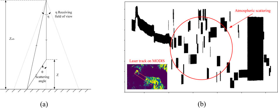
Figure 10. Influence of cloud occlusion on the distribution of photon point cloud data. (a) Influence of atmospheric scatter-ing on satellite laser altimetry. (b) Affected ICESat-2 cases.

5.3 Application prospect of SLA underwater detection

With the development of SLA technology, researchers can use the underwater information obtained by ICESat-2 to address bottleneck issues related to water research. This is reflected in the following three aspects. Firstly, for hydrology and water resource management, SLA technology can be used to accurately monitor the water levels and underwater topography of inland water bodies, such as rivers, lakes, and reservoirs, and to establish more refined hydrological models to simulate target changes (Yang et al., 2023). This is crucial for the rational planning and dispatch of water resources, assessment of reservoir storage capacity, early flood warning, and drought monitoring (Xu et al., 2020). Particularly in remote or hard-to-reach areas, this technology provides a non-contact water level monitoring method, greatly improving the coverage and frequency of hydrological observations. Secondly, for water ecology and water environment research, SLA data can not only be used to measure the depth of water bodies but also to help scientists understand optical properties such as water body transparency and suspended matter content, thereby monitoring and evaluating the water quality status (Zheng et al., 2022). In ecological protection zones and sensitive waters, this technology can track changes in the environment and provide data to support ecological protection and restoration. Thirdly, in the field of oceanography, SLA technology is particularly important for mapping seafloor topography in shallow sea areas. It provides information on the coastal erosion, seabed sediment distribution, and coral reef health (Yu et al., 2021). In addition, this technology is used to monitor sea level rise and fall, ocean surface fluctuations, and tidal changes, providing important data for the establishment and verification of ocean dynamic models.

In summary, SLA technology shows strong application potential in the fields of hydrology, water resource management, aquatic ecology, water environment protection, and oceanography. With the continuous development of technology and expansion of its application scope, this technology is expected to bring deeper research perspectives and more effective management tools to the above fields in the future.

6 Conclusion

At present, there is no clear conclusion regarding the impact of changes in the optical properties of water on the accuracy of SLA data. In view of this, we combined ICESat-2, MODIS, Landsat-8 and situ data to quantify the water quality in the Oahu Island region using AEDTA and RFR methods, and changes in the underwater measurement accuracy. The conclusions are as follows:

1. There was a positive correlation between water quality and water permeability in the spatial distribution, with a correlation coefficient of 0.72. The larger the value of KD490, the smaller the proportion of photons that can penetrate the water sur-face. Among them, Kd490 0.5 is a critical value. When this value is exceeded the number of water-transmitting photons decreases significantly.

2. By combining the strong and weak beams, cross-track, and LIDAR verification data, it was found that the depth measurement accuracy of ICESat-2 strong beams under different water quality conditions was significantly better than that of weak beams. The maximum measurement deviation caused by the multiple scattering of water bodies can reach the meter level. In the future, underwater bathymetry corrections should consider the influence of multiple scattering.

3. The empirical model for water body multiple scattering correction established in this study has a certain correction effect on the data obtained when the water quality, Kd490, is less than or equal to 0.4. However, the model cannot be fully applied when the water becomes more turbid, and it needs to be combined with the mechanism model for an in-depth analysis.

Data availability statement

The original contributions presented in the study are included in the article/supplementary material, further inquiries can be directed to the corresponding author.

Author contributions

QL: Writing – original draft, Conceptualization, Writing – review and editing, Methodology. JW: Investigation, Conceptualization, Writing – review and editing, Supervision. CM: Writing – original draft, Methodology, Conceptualization. HBX: Writing – original draft, Visualization. SZ: Writing – original draft, Visualization. HJX: Writing – original draft, Visualization. FG: Writing – original draft, Visualization. ZZ: Writing – original draft, Visualization.

Funding

The author(s) declare that financial support was received for the research and/or publication of this article. This research was funded by the Tianjin Normal University Research Innovation Project for Postgraduate Students (grant number 2024KYCX114Y) and 2022 Tianjin Municipal Graduate Students’ Scientific Research and Innovation Project (Grant Number 2022SKYZ270).

Acknowledgments

We are grateful to NASA for providing the ATL03 data, and thanks to ATL03 data for their contributions to the related study area. We are grateful to the open-source code AEDTA for supporting this study.

Conflict of interest

The authors declare that the research was conducted in the absence of any commercial or financial relationships that could be construed as a potential conflict of interest.

Generative AI statement

The author(s) declare that no Generative AI was used in the creation of this manuscript.

Publisher’s note

All claims expressed in this article are solely those of the authors and do not necessarily represent those of their affiliated organizations, or those of the publisher, the editors and the reviewers. Any product that may be evaluated in this article, or claim that may be made by its manufacturer, is not guaranteed or endorsed by the publisher.

References

Abdalati, W., Zwally, H. J., Bindschadler, R., Csatho, B., Farrell, S. L., Fricker, H. A., et al. (2010). The ICESat-2 laser altimetry mission. Proc. IEEE 98, 735–751. doi:10.1109/JPROC.2009.2034765

CrossRef Full Text | Google Scholar

Ankerst, M., Breunig, M. M., and Kriegel, H.-P. (1999). OPTICS: ordering points to identify the clustering structure. ACM SIGMOD Record 28, 49–60.

Google Scholar

Ardalan, A. A., Hashemifaraz, A., and Karimi, R. (2023). On the mean sea surface data in the gdr files of the topex/poseidon, jason-1, 2, and 3 missions. Int. Arch. Photogramm. Remote Sens. Spat. Inf. Sci. XLVIII-4/W2-2022, 1–7. doi:10.5194/isprs-archives-XLVIII-4-W2-2022-1-2023

CrossRef Full Text | Google Scholar

Babbel, B. J., Parrish, C. E., and Magruder, L. A. (2021). ICESat-2 elevation retrievals in support of satellite-derived bathymetry for global science applications. Geophys. Res. Lett. 48, e2020GL090629. doi:10.1029/2020GL090629

PubMed Abstract | CrossRef Full Text | Google Scholar

Bergsma, E. W. J., Almar, R., Rolland, A., Binet, R., Brodie, K. L., and Bak, A. S. (2021). Coastal morphology from space: a showcase of monitoring the topography-bathymetry continuum. Remote Sens. Environ. 261, 112469. doi:10.1016/j.rse.2021.112469

CrossRef Full Text | Google Scholar

Caballero, I., and Stumpf, R. P. (2023). Confronting turbidity, the major challenge for satellite-derived coastal bathymetry. Sci. Total Environ. 870, 161898. doi:10.1016/j.scitotenv.2023.161898

PubMed Abstract | CrossRef Full Text | Google Scholar

Carlson, R. E. (1977). A trophic state index for lakes1. Limnol. and Oceanogr. 22, 361–369. doi:10.4319/lo.1977.22.2.0361

CrossRef Full Text | Google Scholar

Chen, L., Letu, H., Fan, M., Shang, H., Tao, J., Wu, L., et al. (2022). An introduction to the Chinese high-resolution earth observation system: gaofen-1∼7 civilian satellites. J. Remote Sens. 2022, 2022–9769536. doi:10.34133/2022/9769536

CrossRef Full Text | Google Scholar

Chen, Y., Le, Y., Zhang, D., Wang, Y., Qiu, Z., and Wang, L. (2021a). A photon-counting LiDAR bathymetric method based on adaptive variable ellipse filtering. Remote Sens. Environ. 256, 112326. doi:10.1016/j.rse.2021.112326

CrossRef Full Text | Google Scholar

Chen, Y., Zhu, Z., Le, Y., Qiu, Z., Chen, G., and Wang, L. (2021b). Refraction correction and coordinate displacement compensation in nearshore bathymetry using ICESat-2 lidar data and remote-sensing images. Opt. Express 29, 2411. doi:10.1364/OE.409941

PubMed Abstract | CrossRef Full Text | Google Scholar

Costa, B. M., Battista, T. A., and Pittman, S. J. (2009). Comparative evaluation of airborne LiDAR and ship-based multibeam SoNAR bathymetry and intensity for mapping coral reef ecosystems. Remote Sens. Environ. 113, 1082–1100. doi:10.1016/j.rse.2009.01.015

CrossRef Full Text | Google Scholar

Cui, Y., Chen, X., Gao, J., Yan, B., Tang, G., and Hong, Y. (2018). Global water cycle and remote sensing big data: overview, challenge, and opportunities. Big Earth Data 2, 282–297. doi:10.1080/20964471.2018.1548052

CrossRef Full Text | Google Scholar

Dong, Y., Liu, Y., Hu, C., and Xu, B. (2019). Coral reef geomorphology of the Spratly Islands: a simple method based on time-series of Landsat-8 multi-band inundation maps. ISPRS J. Photogrammetry Remote Sens. 157, 137–154. doi:10.1016/j.isprsjprs.2019.09.011

CrossRef Full Text | Google Scholar

Hedley, J. D., Velázquez-Ochoa, R., and Enríquez, S. (2021). Seagrass depth distribution mirrors coastal development in the Mexican caribbean – an automated analysis of 800 satellite images. Front. Mar. Sci. 8, 733169. doi:10.3389/fmars.2021.733169

CrossRef Full Text | Google Scholar

Herzfeld, U. C., McDonald, B. W., Wallin, B. F., Neumann, T. A., Markus, T., Brenner, A., et al. (2014). Algorithm for detection of ground and canopy cover in micropulse photon-counting lidar altimeter data in preparation for the ICESat-2 mission. IEEE Trans. Geosci. Remote Sens. 52, 2109–2125. doi:10.1109/TGRS.2013.2258350

CrossRef Full Text | Google Scholar

Kutser, T., Hedley, J., Giardino, C., Roelfsema, C., and Brando, V. E. (2020). Remote sensing of shallow waters – a 50 year retrospective and future directions. Remote Sens. Environ. 240, 111619. doi:10.1016/j.rse.2019.111619

CrossRef Full Text | Google Scholar

Lao, J., Wang, C., Zhu, X., Xi, X., Nie, S., Wang, J., et al. (2021). Retrieving building height in urban areas using ICESat-2 photon-counting LiDAR data. Int. J. Appl. Earth Observation Geoinformation 104, 102596. doi:10.1016/j.jag.2021.102596

CrossRef Full Text | Google Scholar

Leng, Z., Zhang, J., Ma, Y., and Zhang, J. (2023). ICESat-2 bathymetric signal reconstruction method based on a deep learning model with active–passive data fusion. Remote Sens. 15, 460. doi:10.3390/rs15020460

CrossRef Full Text | Google Scholar

Li, G., Guo, J., Tang, X., Ye, F., Zuo, Z., Liu, Z., et al. (2020). Preliminary quality analysis of gf-7 satellite laser altimeter full waveform data. Int. Arch. Photogramm. Remote Sens. Spat. Inf. Sci. XLIII-B1-2020, 129–134. doi:10.5194/isprs-archives-XLIII-B1-2020-129-2020

CrossRef Full Text | Google Scholar

Lu, X., Hu, Y., Omar, A., Yang, Y., Vaughan, M., Lee, Z., et al. (2023). Lidar attenuation coefficient in the global oceans: insights from ICESat-2 mission. Opt. Express 31, 29107. doi:10.1364/OE.498053

PubMed Abstract | CrossRef Full Text | Google Scholar

Lu, X., Hu, Y., Pelon, J., Trepte, C., Liu, K., Rodier, S., et al. (2016). Retrieval of ocean subsurface particulate backscattering coefficient from space-borne CALIOP lidar measurements. Opt. Express 24, 29001. doi:10.1364/OE.24.029001

PubMed Abstract | CrossRef Full Text | Google Scholar

Lu, X., Hu, Y., Yang, Y., Neumann, T., Omar, A., Baize, R., et al. (2021). New Ocean subsurface optical properties from space lidars: CALIOP/CALIPSO and ATLAS/ICESat-2. Earth Space Sci. 8, e2021EA001839. doi:10.1029/2021EA001839

CrossRef Full Text | Google Scholar

Ma, Y., Xu, N., Sun, J., Wang, X. H., Yang, F., and Li, S. (2019). Estimating water levels and volumes of lakes dated back to the 1980s using Landsat imagery and photon-counting lidar datasets. Remote Sens. Environ. 232, 111287. doi:10.1016/j.rse.2019.111287

CrossRef Full Text | Google Scholar

Madson, A., and Sheng, Y. (2021). Automated water level monitoring at the continental scale from ICESat-2 photons. Remote Sens. 13, 3631. doi:10.3390/rs13183631

CrossRef Full Text | Google Scholar

Markus, T., Neumann, T., Martino, A., Abdalati, W., Brunt, K., Csatho, B., et al. (2017). The ice, cloud, and land elevation satellite-2 (ICESat-2): science requirements, concept, and implementation. Remote Sens. Environ. 190, 260–273. doi:10.1016/j.rse.2016.12.029

CrossRef Full Text | Google Scholar

Moudrý, V., Gdulová, K., Gábor, L., Šárovcová, E., Barták, V., Leroy, F., et al. (2022). Effects of environmental conditions on ICESat-2 terrain and canopy heights retrievals in Central European mountains. Remote Sens. Environ. 279, 113112. doi:10.1016/j.rse.2022.113112

CrossRef Full Text | Google Scholar

Narin, O. G., Abdikan, S., Gullu, M., Lindenbergh, R., Balik Sanli, F., and Yilmaz, I. (2024). Improving global digital elevation models using space-borne GEDI and ICESat-2 LiDAR altimetry data. Int. J. Digital Earth 17, 2316113. doi:10.1080/17538947.2024.2316113

CrossRef Full Text | Google Scholar

Neumann, T., Brenner, A., Hancock, D., Robbins, J., Saba, J., Harbeck, K., et al. (2021). ATLAS/ICESat-2 L2A global geolocated photon data. Version 5. doi:10.5067/ATLAS/ATL03.005

CrossRef Full Text | Google Scholar

Ni, M., Xu, N., Ou, Y., Yao, J., Li, Z., Mo, F., et al. (2024). The first 10-m China’s national-scale sandy beach map in 2022 derived from Sentinel-2 imagery. Int. J. Digital Earth 17, 2425163. doi:10.1080/17538947.2024.2425163

CrossRef Full Text | Google Scholar

Parrish, C., Magruder, L., Neuenschwander, A., Forfinski-Sarkozi, N., Alonzo, M., and Jasinski, M. (2019). Validation of ICESat-2 ATLAS bathymetry and analysis of ATLAS’s bathymetric mapping performance. Remote Sens. 11, 1634. doi:10.3390/rs11141634

CrossRef Full Text | Google Scholar

Pedregosa, F., Varoquaux, G., Gramfort, A., Michel, V., Thirion, B., Grisel, O., et al. (2012). Scikit-learn: machine learning in Python. Machine learning in PYTHON. arXiv.

Google Scholar

Peña-Arancibia, J. L., Ticehurst, C. J., Yu, Y., McVicar, T. R., and Marvanek, S. P. (2024). Feasibility of monitoring floodplain on-farm water storages by integrating airborne and satellite LiDAR altimetry with optical remote sensing. Remote Sens. Environ. 302, 113992. doi:10.1016/j.rse.2024.113992

CrossRef Full Text | Google Scholar

Pereira, P., Baptista, P., Cunha, T., Silva, P. A., Romão, S., and Lafon, V. (2019). Estimation of the nearshore bathymetry from high temporal resolution Sentinel-1A C-band SAR data - a case study. Remote Sens. Environ. 223, 166–178. doi:10.1016/j.rse.2019.01.003

CrossRef Full Text | Google Scholar

Schubert, E., Sander, J., Ester, M., Kriegel, H. P., and Xu, X. (2017). DBSCAN revisited, revisited: why and how you should (still) use DBSCAN. ACM Trans. Database Syst. 42, 1–21. doi:10.1145/3068335

CrossRef Full Text | Google Scholar

Schutz, B. E., Zwally, H. J., Shuman, C. A., Hancock, D., and DiMarzio, J. P. (2005). Overview of the ICESat mission. Geophys. Res. Lett. 32, 2005GL024009. doi:10.1029/2005GL024009

CrossRef Full Text | Google Scholar

Tang, X., Gao, X., Cao, H., Mo, F., Wang, Z., Xu, W., et al. (2020a). The China ZY3-03 mission: surveying and mapping technology for high-resolution remote sensing satellites. IEEE Geosci. Remote Sens. Mag. 8, 8–17. doi:10.1109/MGRS.2019.2929770

CrossRef Full Text | Google Scholar

Tang, X., Xie, J., Liu, R., Huang, G., Zhao, C., Zhen, Y., et al. (2020b). Overview of the GF-7 laser altimeter system mission. Earth Space Sci. 7, e2019EA000777. doi:10.1029/2019EA000777

CrossRef Full Text | Google Scholar

Tang, X., Yao, J., Chen, J., Li, G., and Zhang, W. (2022). Multimodel fusion method for cloud detection in satellite laser footprint images. IEEE Geosci. Remote Sens. Lett. 19, 1–5. doi:10.1109/LGRS.2022.3192067

CrossRef Full Text | Google Scholar

Tilstone, G. H., Pardo, S., Dall’Olmo, G., Brewin, R. J. W., Nencioli, F., Dessailly, D., et al. (2021). Performance of ocean colour chlorophyll a algorithms for sentinel-3 OLCI, MODIS-aqua and suomi-VIIRS in open-ocean waters of the atlantic. Remote Sens. Environ. 260, 112444. doi:10.1016/j.rse.2021.112444

CrossRef Full Text | Google Scholar

Wang, B., Ma, Y., Zhang, J., Zhang, H., Zhu, H., Leng, Z., et al. (2023a). A noise removal algorithm based on adaptive elevation difference thresholding for ICESat-2 photon-counting data. Int. J. Appl. Earth Observation Geoinformation 117, 103207. doi:10.1016/j.jag.2023.103207

CrossRef Full Text | Google Scholar

Wang, F., Wang, Y., Zhang, K., Hu, M., Weng, Q., and Zhang, H. (2021). Spatial heterogeneity modeling of water quality based on random forest regression and model interpretation. Environ. Res. 202, 111660. doi:10.1016/j.envres.2021.111660

PubMed Abstract | CrossRef Full Text | Google Scholar

Wang, J., Xie, X., Deng, R., Li, J., Tang, Y., Liang, Y., et al. (2023b). Improved the impact of SST for HY-2A scatterometer measurements by using neural network model. Sensors (Basel). 23, 4825. doi:10.3390/s23104825

PubMed Abstract | CrossRef Full Text | Google Scholar

Wen, Z., Tang, X., Ai, B., Yang, F., Li, G., Mo, F., et al. (2024a). A new extraction and grading method for underwater topographic photons of photon-counting LiDAR with different observation conditions. Int. J. Digital Earth 17, 1–30. doi:10.1080/17538947.2023.2295985

CrossRef Full Text | Google Scholar

Wen, Z., Tang, X., Li, G., Ai, B., Wang, G., Yao, J., et al. (2024b). Sea surface signal extraction for photon-counting LiDAR data: a general method by dual-signal unmixing parameters. IEEE J. Sel. Top. Appl. Earth Obs. Remote Sens. 17, 428–437. doi:10.1109/JSTARS.2023.3329962

CrossRef Full Text | Google Scholar

Xu, N., Lu, H., Li, W., and Gong, P. (2024a). Natural lakes dominate global water storage variability. Sci. Bull. 69, 1016–1019. doi:10.1016/j.scib.2024.02.023

PubMed Abstract | CrossRef Full Text | Google Scholar

Xu, N., Ma, X., Ma, Y., Zhao, P., Yang, J., and Wang, X. H. (2021a). Deriving highly accurate shallow water bathymetry from sentinel-2 and ICESat-2 datasets by a multitemporal stacking method. IEEE J. Sel. Top. Appl. Earth Obs. Remote Sens. 14, 6677–6685. doi:10.1109/JSTARS.2021.3090792

CrossRef Full Text | Google Scholar

Xu, N., Ma, Y., Wei, Z., Huang, C., Li, G., Zheng, H., et al. (2022a). Satellite observed recent rising water levels of global lakes and reservoirs. Environ. Res. Lett. 17, 074013. doi:10.1088/1748-9326/ac78f8

CrossRef Full Text | Google Scholar

Xu, N., Ma, Y., Zhang, W., and Wang, X. H. (2021b). Surface-water-level changes during 2003–2019 in Australia revealed by ICESat/ICESat-2 altimetry and Landsat imagery. IEEE Geosci. Remote Sens. Lett. 18, 1129–1133. doi:10.1109/LGRS.2020.2996769

CrossRef Full Text | Google Scholar

Xu, N., Ma, Y., Zhang, W., Wang, X. H., Yang, F., and Su, D. (2020). Monitoring annual changes of lake water levels and volumes over 1984–2018 using Landsat imagery and ICESat-2 data. Remote Sens. 12, 4004. doi:10.3390/rs12234004

CrossRef Full Text | Google Scholar

Xu, N., Ma, Y., Zhou, H., Zhang, W., Zhang, Z., and Wang, X. H. (2022b). A method to derive bathymetry for dynamic water bodies using ICESat-2 and GSWD data sets. IEEE Geosci. Remote Sens. Lett. 19, 1–5. doi:10.1109/LGRS.2020.3019396

CrossRef Full Text | Google Scholar

Xu, N., Wang, L., Zhang, H.-S., Tang, S., Mo, F., and Ma, X. (2024b). Machine learning based estimation of coastal bathymetry from ICESat-2 and sentinel-2 data. IEEE J. Sel. Top. Appl. Earth Obs. Remote Sens. 17, 1748–1755. doi:10.1109/JSTARS.2023.3326238

CrossRef Full Text | Google Scholar

Xu, Y., Cao, B., Deng, R., Cao, B., Liu, H., and Li, J. (2023). Bathymetry over broad geographic areas using optical high-spatial-resolution satellite remote sensing without in-situ data. Int. J. Appl. Earth Observation Geoinformation 119, 103308. doi:10.1016/j.jag.2023.103308

CrossRef Full Text | Google Scholar

Yang, H., Qiao, B., Huang, S., Fu, Y., and Guo, H. (2023). Fitting profile water depth to improve the accuracy of lake depth inversion without bathymetric data based on ICESat-2 and Sentinel-2 data. Int. J. Appl. Earth Observation Geoinformation 119, 103310. doi:10.1016/j.jag.2023.103310

CrossRef Full Text | Google Scholar

Yang, Y., Marshak, A., Varnai, T., Wiscombe, W., and Yang, P. (2010). Uncertainties in ice-sheet altimetry from a spaceborne 1064-nm single-channel lidar due to undetected thin clouds. IEEE Trans. Geosci. Remote Sens. 48, 250–259. doi:10.1109/TGRS.2009.2028335

CrossRef Full Text | Google Scholar

Yao, J., Mo, F., Xu, N., Ma, C., Wang, M., Xia, H., et al. (2025). The Chinese Laser Altimetry Satellite will significantly enhance the 3D mapping capability of global coastal zones. TIG 3, 100121. doi:10.59717/j.xinn-geo.2024.100121

CrossRef Full Text | Google Scholar

Yao, J., Tang, X., Li, G., Chen, J., Zuo, Z., Ai, B., et al. (2021a). Influence of atmospheric scattering on the accuracy of laser altimetry of the GF-7 satellite and corrections. Remote Sens. 14, 129. doi:10.3390/rs14010129

CrossRef Full Text | Google Scholar

Yao, J., Tang, X., Li, G., Guo, J., Chen, J., Yang, X., et al. (2021b). Cloud detection of GF-7 satellite laser footprint image. IET Image Process. 15, 2127–2134. doi:10.1049/ipr2.12141

CrossRef Full Text | Google Scholar

Yu, Y., Sandwell, D. T., Gille, S. T., and Villas Bôas, A. B. (2021). Assessment of ICESat-2 for the recovery of ocean topography. Geophys. J. Int. 226, 456–467. doi:10.1093/gji/ggab084

CrossRef Full Text | Google Scholar

Zheng, H., Ma, Y., Huang, J., Yang, J., Su, D., Yang, F., et al. (2022). Deriving vertical profiles of chlorophyll-a concentration in the upper layer of seawaters using ICESat-2 photon-counting lidar. Opt. Express 30, 33320. doi:10.1364/OE.463622

PubMed Abstract | CrossRef Full Text | Google Scholar

Zheng, Z., Huang, C., Li, Y., Lyu, H., Huang, C., Chen, N., et al. (2023). A semi-analytical model to estimate Chlorophyll-a spatial-temporal patterns from Orbita Hyperspectral image in inland eutrophic waters. Sci. Total Environ. 904, 166785. doi:10.1016/j.scitotenv.2023.166785

PubMed Abstract | CrossRef Full Text | Google Scholar

Zuo, Z., Tang, X., Li, G., Ma, Y., Zhang, W., and Li, S. (2021). Inversion of terrain slope and roughness with satellite laser altimeter full-waveform data assisted by shuttle radar topographic mission. Remote Sens. 13, 424. doi:10.3390/rs13030424

CrossRef Full Text | Google Scholar