Unveiling spatiotemporal evolution and driving factors of ecosystem service value: interpretable HGB-SHAP machine learning model

Introduction: The ecosystem service value (ESV) is a critical element in the preservation of ecological barriers. The objective of this study is to elucidate the nonlinear correlation between ESV and the key factors that contribute to enhancing the accuracy and reliability of ecosystem service value assessment.

Methods: In this study, ESV were evaluated based on grid and county scales. Furthermore, the driving factors of ESV were explored using the explainable machine learning method.

Results: The findings are as follows: (1) The net ESV of the Gangjiang Upstream Basin (GUB) has undergone a decline from 1990 to 2000, with climate regulation and hydrological regulation collectively accounting for approximately 50% of all functions. (2) A mere 0.69% of the areas exhibited an increase in the level of ESV, while 11.19% demonstrated a decline by 2020, based on the grid scale. The ESV exhibited a slight increase in two counties, while it demonstrated a decrease in the remaining 16 counties at the county scale. The ESV exhibited a substantial positive spatial correlation, manifesting as the presence of considerable high-high and low-low clustering regions. (3) The interpretable machine learning analysis revealed a consistently strong negative correlation between ESV and human activity intensity (HAI), fractional vegetation cover (FVC), and elevation across the entire observed range. In contrast, the soil organic matter (SOC) demonstrated a non-linear, highly significant positive correlation with ESV.

Discussion: This paper addresses the observed decline in the value of ecosystem services of GUB by proposing a series of strategies designed to enhance ESV in the region. Furthermore, drawing on research findings related to the driving factors and thresholds of ESV, this paper presents specific measures that can serve as references for managers.

1 Introduction

China has suggested the grand strategy of developing a “Beautiful China” in response to the growing ecological and environmental issues brought on by rapid urbanization. This plan specifically aims to “support high-quality development with a high-quality ecological environment.” As a result, ecosystem services have gradually become a hot spot (Zhang et al., 2021). The goods and services that are obtained either directly or indirectly from ecosystem functions are known as ecosystem services. They consist of energy flows, material flows and information flows from natural and non-natural capital that contribute to human wellbeing. Changes in ecosystem services are closely linked to human welfare (Wang et al., 2017; Ouyang et al., 1999). In 1997, Costanza et al. published a paper in Nature on the global assessment of ESV, which stimulated research in the field of ecosystem services (Costanza et al., 1997). Xie Gaodi et al. developed the “Equivalent Factor Table for Ecosystem Service Value in China,” which was tailored to the specific characteristics of ecosystems and has been widely utilized in studies of ESV at various regional scales (Xie et al., 2015; Liu et al., 2021; Gao et al., 2021). One of the main ways that human activity affects ecosystems is through land use change (LUC). This is because LUC modifies the availability of ecosystem services and products, which impacts ecosystem patterns and functions. Consequently, land use change plays a pivotal role in ecosystem service value (Xiao et al., 2020; Yang X. et al, 2025). Rapid growth over the last 3 decades has exacerbated changes in land use, including as reclamation, urbanization, and land abandonment, which has led to a fall in ESV and a degradation of ecosystem service functions. This has posed a significant challenge to regional sustainable development (Sun et al., 2024; Liu J. et al., 2014).

Numerous national and international studies have examined the impact of LUC on ecosystem service value. The unit area value equivalent factor method, the integrated model method, and the remote sensing quantification method are some evaluation techniques used in ESV assessment (Zhang and Fu, 2014; Zhang et al., 2024; Wang et al., 2024). The evolution features, response relationships, and driving forces of LUC-ESV have been the subject of a considerable number of investigations on a large scale. One of the scales selected for investigation was grid units, another was administrative regions, and a third was watersheds (Wei et al., 2023; Shen et al., 2024; Wang et al., 2021). Furthermore, to illustrate how LUC affects ESV, current research mostly uses quantitative techniques, such as hotspot analysis, land use transition matrices, land use change maps, and horizontal changes in land use types (Ye et al., 2004; Feng et al., 2021). Nevertheless, there is still little study on multi-scale studies. Therefore, this study reveals the multi-dimensional characteristics of ESV based on grid and county scales.

To improve regional ecological security and support the sustainable growth, it is essential to determine the variables that drive ESV. However, conventional quantitative techniques that concentrate on explanatory analysis, like spatial quantile regression modeling, geographically weighted regression, and geographic detector, are limited in their ability to handle nonlinear interactions and the physical significance of the driving factors (Shi et al., 2022; Zhang et al., 2023; Deng et al., 2025). Geodetector analysis identifies the factors driving spatial heterogeneity in ESV and can reveal both dominant drivers and their optimal combinations. However, given the adoption of disparate criteria and rules for factor selection and data discretization by researchers, the final detection results may exhibit variability to a certain extent (Wang et al., 2025). Machine learning (ML) algorithms provide innovative tools for clarifying intricate driving mechanisms and accurate prediction in order to handle this problem (Zhao et al., 2025). A more realistic depiction of the underlying dynamics is possible thanks to machine learning’s ability to capture the interactions between variables and their combined impacts on ESV (Li et al., 2025a). Both natural and man-made elements contribute to the intricate construction process of ecosystem structure and function services (Yang Y. et al., 2025). ML methods, with their powerful nonlinear modeling capabilities, offer novel analytical tools for ESV research (Li et al., 2025b). However, decision-makers face interpretability issues due to the “black box” nature of ML models, which makes it difficult for them to intuitively understand the relative relevance of driving elements (Lee et al., 2022). In comparison with conventional factor-analysis methodologies, Shapley Additive Explanations (SHAP) enhances model transparency while preserving predictive accuracy, thereby elucidating the key drivers and their underlying mechanisms. The integration of feature importance, partial dependence plots, and SHAP values within the framework of ML and SHAP offers a comprehensive analysis of the impact of drivers on ecosystem services (Zhao et al., 2022; Huang et al., 2025). This enables researchers to visualize the interactions between components and their overall impacts, as well as to comprehend the direction (positive or negative) and size of impact (Ling et al., 2022).

The GUB, which includes 18 counties in Ganzhou Municipality, is located in the southern part of Jiangxi Province, China. The GUB represents the source area for both the Ganjiang River and the Dongjiang River. The Ganjiang River represents the largest river system in the Poyang Lake Basin and constitutes a pivotal tributary of the lower Yangtze River. Additionally, the region of GUB was a crucial barrier for ecological security in southern China. The GUB is located within Ganzhou City, where confirmed ion-adsorption rare-earth reserves total approximately 470 thousand tonnes-approximately 40% of China’s total ionic-type rare earth resources. This has led to the region being dubbed the “Rare Earth Kingdom” (Xiong et al., 2019). However, due to human activity, the area is experiencing serious environmental problems that are significantly affecting the composition and functionality of the local ecosystem. In light of the aforementioned background, the present study puts forth the two hypotheses to direct the investigation. Firstly, the ESV of GUB has undergone a substantial spatiotemporal decline over the past 2 decades, primarily attributable to LUC and HAI. Secondly, the relationship between ESV and driving factors is nonlinear and scale-dependent, and traditional linear models are insufficient to capture these complex interactions. Accordingly, explainable machine learning approach is applied to explore the driving factors of ESV. The study aims to: (1) Investigate the spatiotemporal changes of ESV. (2) Optimal machine learning model selection via parameter comparison. (3) Detect the driving factor of ESV. The findings will furnish theoretical backing and consultancy expertise for the zonal administration of ecosystem services of the GUB, thereby contributing to the advancement of the “Ganzhou Model” of a Beautiful China.

2 Materials and methods

2.1 Study area

The GUB is situated in the upper reach of the Ganjiang River (Figure 1), in Jiangxi Province, southern China, encompassing 18 counties of Ganzhou city. It is situated between latitudes 24°29′N and 27°09′N, and longitudes 113°54′E and 116°38′E, encompassing a total area of 39,379.64 km², which constitutes 23.6% of the total area of Jiangxi Province. The region’s topography is predominantly characterised by mountainous and hilly terrain, which collectively constitute the geomorphological framework and account for 80.98% of the total area. The GUB has a subtropical monsoon climate because it is located on the southern border of the mid-subtropical zone. The predominant winter and summer monsoons, heavy spring and summer precipitation, clear seasonal variations, a moderate temperature, copious amounts of heat and precipitation, brief episodes of extreme cold or heat, and an extended frost-free season are its defining features. The average annual temperature in the area is 19.8°C, while the average annual precipitation is 1,318.9 mm (Xu, 2025).

Figure 1

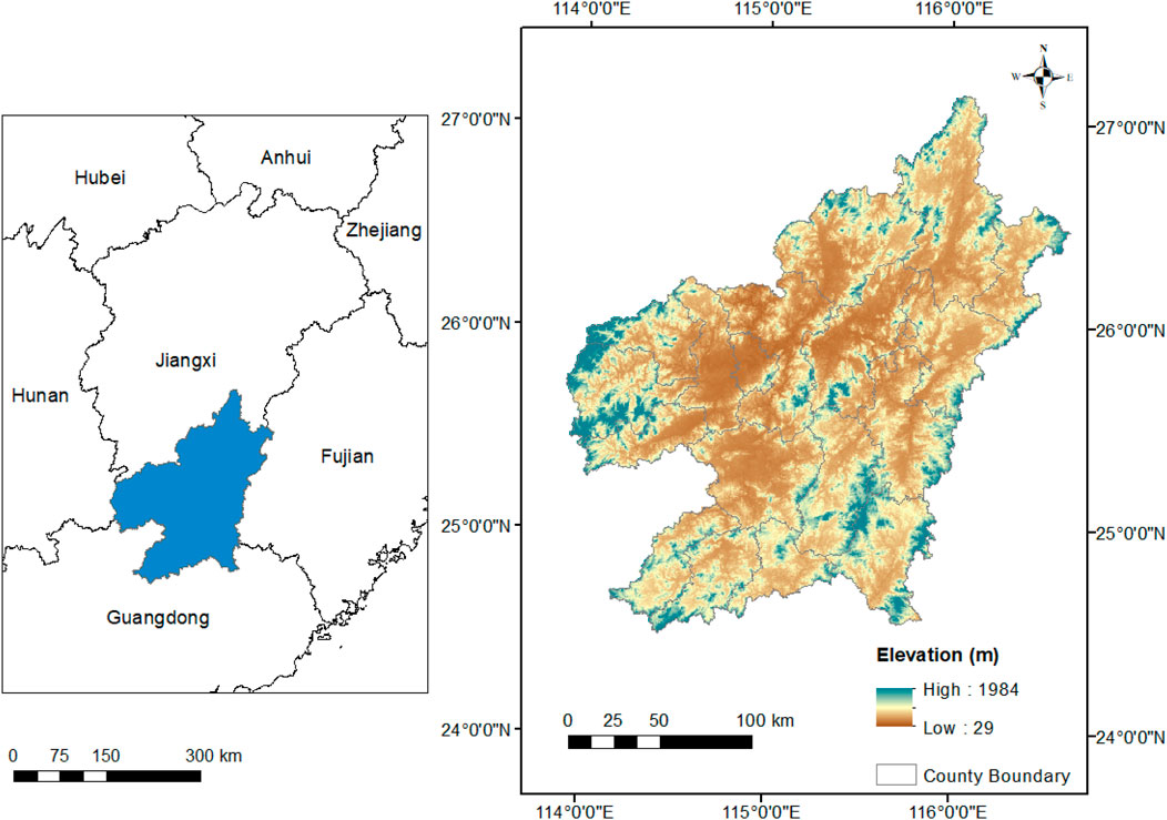
Figure 1. Geographic location of study area.

2.2 Data sources

The data comprised digital elevation model (DEM), land use data, Soil Organic Carbon (SOC) and grain output (Table 1). The grain output and GDP data were provided by the Ganzhou Municipal Bureau of Statistics (2021), while the product price data was sourced from the China Agricultural Products Price Survey Yearbook (2021). The research framework is shown in Figure 2. In order to standardize the spatial resolution of multi-source data, the present study employed resampling techniques to normalize the raw data. The study area was meticulously delineated into a regular grid of 5 km × 5 km cells. The mean value of all data points within each grid cell was calculated using spatial statistical methods, and these means were used as training samples for the machine learning model.

Table 1

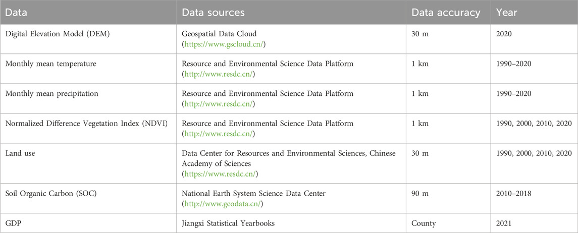
Table 1. Data source.

Figure 2

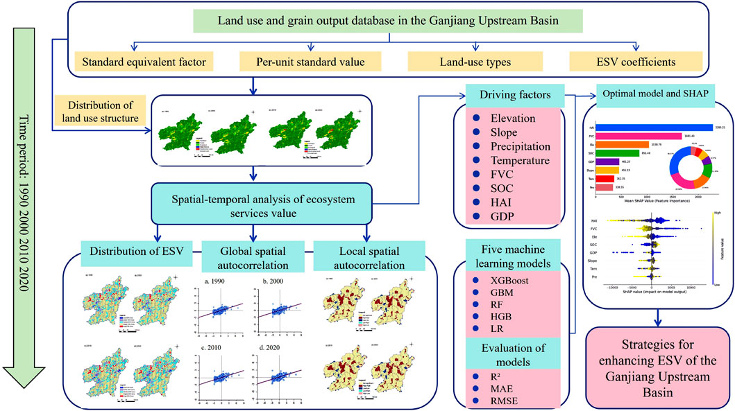
Figure 2. The research framework.

2.3 Method for assessing ESV

In this study, the equivalent factor method was employed to ascertain the value of individual ecosystem service equivalent factors and to estimate the coefficients for different land use types (Xie et al., 2003). According to data from the Ganzhou Statistical Yearbook, In 2020, the average grain production per unit area of the GUB was 9,792.71 kg/hm². Considering that the research duration extended over 3 decades, the fixed price of 2020 was utilized to correlate the ESV of each period. The principal crops cultivated in the GUB are rice, vegetables, and fungi, along with oil crops. The mean prices for rice, vegetables, fungi, and oil crops in 2020 were 3.53 yuan/kg, 2.29 yuan/kg, 4.7 yuan/kg, and 2.21 yuan/kg, respectively. Thus, in 2020, the economic value of the equivalent factor of the GUB was 4,109.01 yuan/hm², which allowed for the calculation of the ESV coefficients for the GUB (Table 2). The calculation of ESV is shown in Equations 1, 2 (Hu et al., 2023; Shi et al., 2012):

$ESV=\sum \left(A_k\times V{C}_k\right)(1)$

${ESV}_k=\sum \left(A_k\times V{C}_{fk}\right)(2)$

Table 2

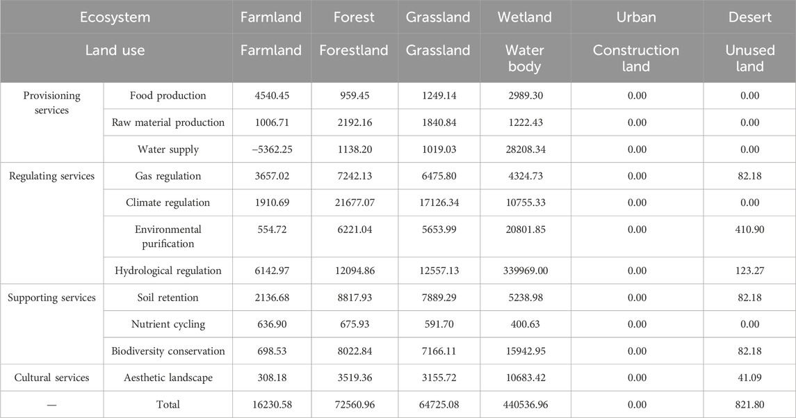
Table 2. Coefficients of ESV of different land use of the GUB, 2020. (yuan/hm²).

Where ESV represents the total value of ecosystem services, $V{C}_k$ is the ecosystem value coefficient, $A_k$ is the area of land use type k, $ES{V}_k$ is the value of the fth ecosystem service function, and $V{C_f}_k$ is the value coefficient of the fth service function for land use type k.

2.4 Grid-based spatial expression of ESV

Grids measuring 2 km by 2 km, 5 km by 5 km, 8 km by 8 km, and 10 km by 10 km were first built as potential assessment units for this study. The ArcGIS10.8 software tools, including Create Fishnet, Clip, and Dissolve, were employed to select a grid size of 5 km × 5 km, resulting in a total of 1,744 small grids. Based on the land use data available for each grid, the ESV (ESV) of each land use within each grid was calculated, and the values were then summed to obtain the total ESV for the grid. The following Equations 3, 4 provide the formula (Li et al., 2018; Yang et al., 2022):

$ES{V}_n=\sum \left(S_{mn}\times L{U}_m\right)(3)$

$ESV={\displaystyle \sum _{n=1}^k}ES{V}_n(4)$

ESV_n represents the ESV (ESV) of the nth land use type within each grid cell; S_mn denotes the area (in hectares) of the nth land use type in the mth grid cell; LU_m is the ESV coefficient for the mth land use type; and k is the total number of land use types.

2.5 Analysis of regional variability based on administrative unit

The regional variability of ESV can be reflected by utilising the relative change rate, as expressed by the following Equation 5 (Liu G. et al., 2014):

$R=\frac{R_L}{R_C}=\frac{\frac{L_b-L_a}{L_a}}{\frac{C_b-C_a}{C_a}}(5)$

R represents the relative change rate, where R_L and R_C are the regional and global change rates, respectively; L_a and L_b denote the initial and final values of regional ESV; and C_a and C_b represent the initial and final values of global ESV. The relative change rate exhibits the following characteristics:

(1) It has been demonstrated that when the relative change rate is greater than or equal to 0, regional ESV trends exhibit alignment with global trends. When the relative change rate is greater than or equal to 0 but less than 1, regional change is weaker. In contrast, a relative change rate that is greater than 1 indicates that regional change exceeds global change.

(2) Conversely, a negative relative change rate, defined as a value less than zero, signifies that regional ESV trends are in opposition to global ESV trends. Specifically, when the rate is between −1 and 0, regional change is weaker than global change; when the rate is less than −1, regional change exceeds global change in magnitude.

2.6 Analysis of spatial autocorrelation

“Spatial autocorrelation” refers to both local and global types of spatial autocorrelation. The global Moran’s index (Moran’sI) is employed to delineate the prevailing trend of spatial correlation in ESV. The local spatial autocorrelation index, represented by Moran’sI_i, reflects the degree of spatial autocorrelation within grid cells (Pearson, 2002). The formula is presented in Equations 6-8 as follow (Jin et al., 2020; Yao et al., 2015):

$Mora{n}^{\prime }sI=\frac{n{\displaystyle {\sum }_{i=1}^n}{\displaystyle {\sum }_{j=1}^n}{w}_{ij}\left(x_i-\overline{x}\right)\left(x_j-\overline{x}\right)}{\left({\displaystyle {\sum }_{i=1}^n}{\displaystyle {\sum }_{j=1}^n}{w}_{ij}\right){\displaystyle {\sum }_{i=1}^n}{\left(x_i-\overline{x}\right)}^2}(6)$

$Mora{n}^{\prime }s{I}_i=\frac{\left(x_i-\overline{x}\right)}{m_0}{\displaystyle \sum _{j=1}^n}{w}_{ij}\left(x_j-\overline{x}\right)(7)$

$m{\dot{}}_0=\frac{{\displaystyle {\sum }_{i=1}^n}{\left(X_i-\overline{x}\right)}^2}{n}(8)$

Where n represents the number of spatial units; $x_i$ and $x_j$ denote the ESV values of the ith and jth spatial units, respectively; x is the mean ESV; $w_{ij}$ is the spatial weight matrix; and ${\dot{m}}_0$ denotes the variance.

2.7 Driving factor analysis of ESV

In this study, a 5 km × 5 km grid was employed to subdivide the study area into 1,744 grid cells, and the mean values of environmental variables within each grid were extracted as feature data. Subsequent to the collection of these data, five machine learning models are constructed, including eXtreme Gradient Boosting (XGBoost), Gradient Boosting Machine (GBM), Random Forest (RF), HistGradientBoosting (HGB), and Linear Regression (LR), to predict ESV. Table 3 offers a synopsis of the fundamental assumptions and the applicable scopes of the five models utilized in this study for ESV prediction. The transition from linear benchmark (LR) to tree-based models facilitates a comprehensive comparison chain, thereby enabling the validation of nonlinear gains. The algorithms RF, GBM, XGBoost, and HGB do not prespecify functional forms, a property that enables them to capture nonlinearities, interactions, and threshold effects between ESV and multisource drivers. The XGBoost and HGB models have been demonstrated to be effective tools for the analysis of large, high-dimensional datasets, with the capacity to meet the demands of multi-scale ESV mapping (Chen and Guestrin, 2016; Ke et al., 2017; Zhang et al., 2020).

Table 3

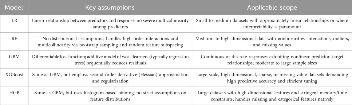
Table 3. The fundamental assumptions and the applicable scopes of ML models.

The dependent variable in this study was ESV, and the independent variables included six natural factors, elevation (Ele), slope, precipitation (Pre), temperature (Tem), soil organic carbon (SOC) and fractional vegetation cover (FVC), and two socioeconomic factors, human activity intensity (HAI) and gross domestic product (GDP). The distributions of the eight variation are shown in Figure 3 (The elevation is shown in Figure 1). To quantify the effect of each factor on ESV, the study incorporated the SHAP analysis method. The dataset was split into two parts randomly: a test set and a training set. The percentage of the former to the latter was 20% and 80%, respectively. The performance of the model was evaluated based on the coefficient of determination (R²), the mean absolute error (MAE), and the root mean square error (RMSE). The optimal model is applied to the trained model for driving factor detection.

Figure 3

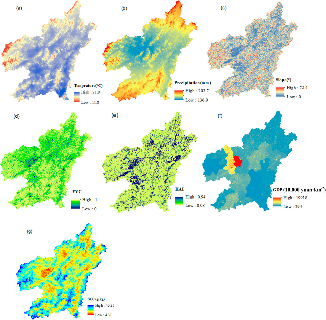
Figure 3. The spatial distribution of driving factors. (a) Temperature, (b) Precipitation, (c) Slope, (d) FVC, (e) HAI, (f) GDP, (g) SOC. Note: human activity intensity (HAI), fractional vegetation cover (FVC), gross domestic product (GDP) and soil organic carbon (SOC).

The extraction of elevation and slope data was conducted using DEM, while the calculation of the FVC and HAI indicators was informed by relevant literature.

The calculation of FVC are shown in Equation 9 (Li et al., 2021):

$FVC=\frac{NDVI-NDV{I}_{\min }}{NDV{I}_{\max }-NDV{I}_{\min }}(9)$

In the formula, FVC represents the vegetation cover (%), NDVI is the normalized difference vegetation index, with the multi-year monthly average used in this study. The NDVI value of pixels that are fully covered by vegetation is known as NDVI_max, whereas the NDVI value of bare soil or regions devoid of vegetation cover is known as NDVI_min.

The HAI was employed to quantify the intensity of human interference in a specific region’s landscape. The HAI value ranged from 0 to 1, with higher values indicating greater human activity impact on the landscape components. The formulas are shown in Equation 10 (Yan et al., 2014):

$HAI={\displaystyle \sum _{i=1}^N}\frac{A_i{P}_i}{TA}(10)$

Where, HAI is the comprehensive index of anthropogenic impacts, N is the number of landscape types, Ai is the area of the ith type of landscape, P_i is the intensity coefficient of anthropogenic impacts of the ith type of landscape, the P_i in this study were given values of 0.12, 0.61, 0.09, 0.12, 0.94, and 0.08 for forestland, farmland, grassland, water body, construction land, and unused land, respectively, based on results of other studies (Yan et al., 2014). TA is the total area of the landscape.

In this study, Pearson’s correlation coefficient was employed to evaluate the relationship between each factor and SHAP values. In order to more accurately depict the nonlinear relationship between the eigenfactors and SHAP values, the LOWESS (locally weighted scatter smoothing) method was introduced to smooth the data. SHAP (SHapley Additive exPlanations) is a game theory-based method for interpreting machine learning models. The methodology employed entails the quantification of the marginal contribution of each input feature variable to the prediction results of individual samples through the utilization of Shapley values (Dandolo et al., 2023). This approach not only elucidates the trend of model predictors but also underscores the significance of features. The following mathematical expressions in Equation 11 are pertinent to this discussion (Aas et al., 2021):

$y_i=y_{base}+f\left(x_{i,1}\right)+f\left(x_{i,2}\right)+\cdots +f\left(x_{i,j}\right)+\cdots f\left(x_{i,k}\right)(11)$

In this equation, y_i denotes the predicted ESV value of the ith sample, y_base signifies the mean ESV prediction of all samples, x_i represents the observed ESV value of the ith sample, f (x_i,j) is the SHAP value of the jth feature of the ith sample, and k denotes the number of input features.

In this study, the Bootstrap method is employed to analyze the uncertainty in the prediction results of SHAP values. Specifically, the generation of multiple Bootstrap samples is achieved through the implementation of 100 resampling with put-back from the original sample. For each Bootstrap sample, the corresponding statistic is computed, thereby estimating the probability distribution of the original statistic. Consequently, we are equipped to derive confidence intervals for the raw statistic. In this context, 95% confidence intervals are delineated by referencing the 2.5% and 97.5% quantiles of the Bootstrap sample statistic. The width of the confidence interval is a critical metric for evaluating the precision of the estimate. Narrower confidence intervals are indicative of precise estimates, while wider intervals suggest greater uncertainty (Sothe et al., 2022). The Bootstrap method has been demonstrated to effectively quantify the uncertainty of the prediction results of SHAP values, thereby providing a more reliable basis for model interpretive analysis.

As demonstrated in the following section, partial dependence plots facilitate a more thorough elucidation of the specific association patterns between each feature and the target variable. The intersection of the dashed line (SHAP = 0) with the LOWESS trend line delineates the SHAP values into two regimes: values above the dashed line (SHAP >0) indicate a positive influence of the driver on ESV, whereas values below the dashed line (SHAP <0) denote an inhibitory effect (Lu et al., 2025).

3 Results

3.1 Analysis of LUC of the GUB

Figure 4 illustrates the distribution of landscape types in GUB in 1990 (a), 2000 (b), 2010 (c), and 2020 (d). Table 4 presents a summary of the observed changes in these landscape types. The findings indicated that forestland has remained the predominant landscape type in GUB, encompassing over 74% of the total area. From 1990 to 2020, the area of forestland exhibited a reduction of 388.19 km². The second-largest landscape type, farmland, exhibited relatively stable conditions. Even while construction land made up a very small percentage of the total area (less than 2%), this category had grown significantly, with a net gain of 363.97 km², or 105.21%. The area of water bodies increased by 12.86 km², while the area of grassland increased by 15.01 km². Unused land exhibited a general decreasing trend, with a small proportion throughout the study period, remaining consistently below 0.1%.

Figure 4

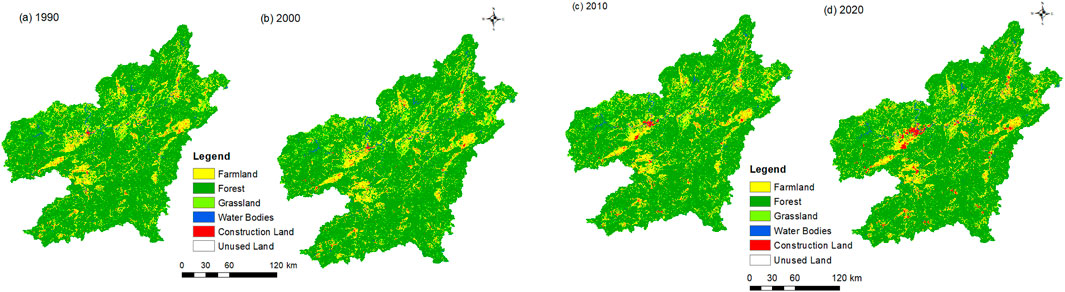
Figure 4. Distribution of LUC of the GUB, 1990–2020. (a) 1990, (b) 2000, (c) 2010, (d) 2020.

Table 4

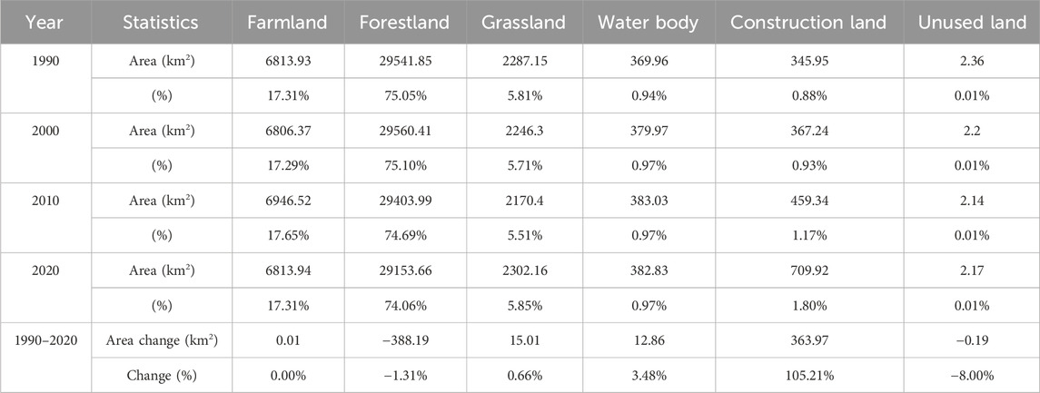
Table 4. LUC characteristics of the GUB, 1990–2020.

3.2 Temporal changes of ESV of the GUB

3.2.1 Analysis of ESV evolution by land use type

The ESV of the GUB exhibited a trend of initial increase followed by a decrease, resulting in a net reduction of 21.5 × 10⁸ yuan (Table 5). Among the various land use types, forestland contributed the most to the overall ESV, accounting for over 83% of the total. This proportion is significantly higher than that of other landscape types. However, the proportion of forestland has shown a declining trend. Water bodies were the second most significant contributor to the ESV, representing over 6% of the total. The ESV of water bodies demonstrated a net increase of 5.67 × 10⁸ yuan. The grassland category exhibited an initial decline, followed by an increase. The ESV of farmland remained unchanged. The contribution of unused land was insignificant, accounting for less than 0.01% of the total value. Furthermore, the ESV of constructed land was not identified.

Table 5

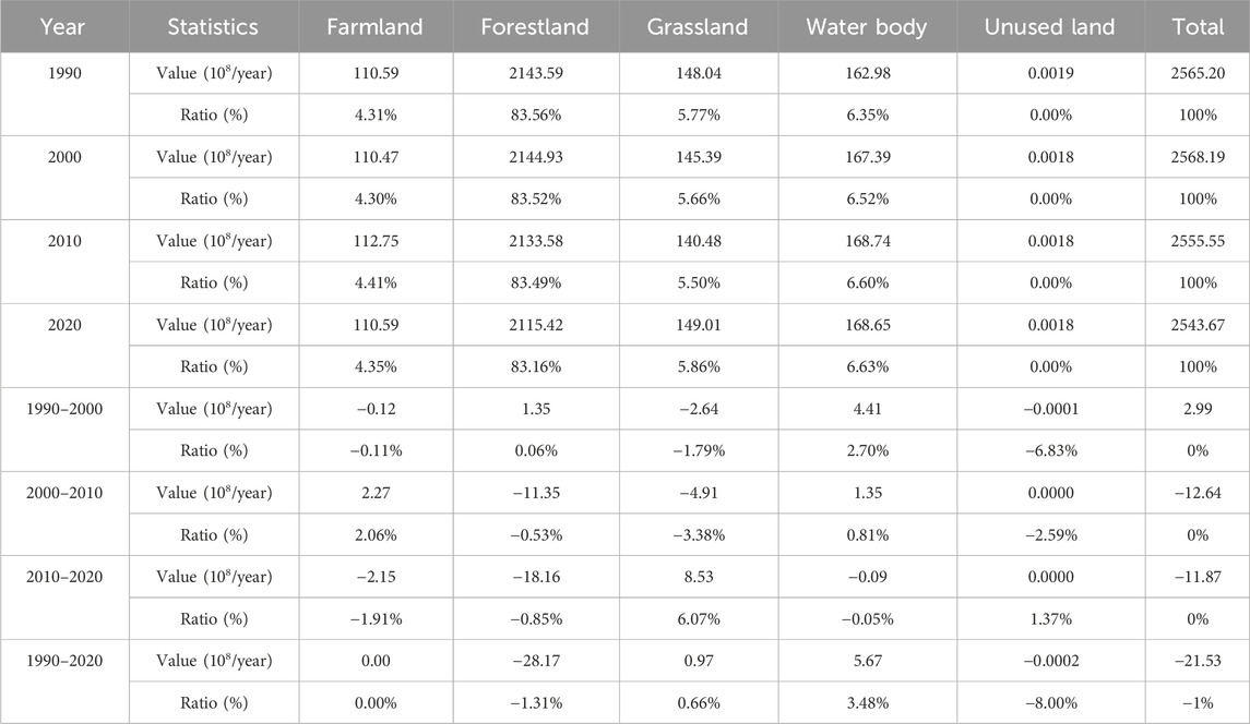
Table 5. Temporal change of ESV of different land use of the GUB, 1990–2020.

3.2.2 Analysis of the value by ecosystem services function

Figure 5 illustrates the value of ecosystem services by function. It is evident that regulating services represent the dominant ecosystem functions of the GUB, significantly surpassing other functions. The two most important factors, climate regulation and hydrological regulation, together make up almost half of the total value. Soil conservation and biodiversity consistently occupy the third and fourth positions, respectively, while supporting services are also significant ecosystem functions in the region, following regulating services.

Figure 5

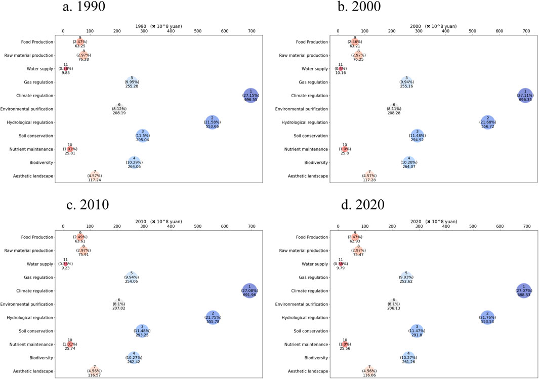
Figure 5. Temporal change of ESV by function of the GUB, 1990–2020. Note: The horizontal axis showed the ESV of individual function, the vertical axis showed the types of individual function. The comparison included the ranking, percentage (%), and value (×10⁸ yuan). (a) 1990, (b) 2000, (c) 2010, (d) 2020.

With regard to the trend in the proportion of service values, there is an overall decline in the values attributed to raw material production, climate regulation, soil conservation, gas regulation, and nutrient cycling. Conversely, the trends observed in environmental purification, hydrological regulation, biodiversity, and aesthetic landscape values indicate an initial increase, followed by a subsequent decrease. The patterns observed in food production and water supply demonstrate fluctuations.

3.3 Spatial variation of ESV based on grid scale

The natural breaks method was utilised for the classification of the ESV index (ESVI) across the various grids into five distinct categories. The categories are ordered from low to high as follows: The categories are defined as follows: low (ESVI ≤24000 yuan/hm²), lower (24000 yuan/hm² < ESVI ≤48000 yuan/hm²), central (48000 yuan/hm² < ESVI ≤64000 yuan/hm²), higher (64000 yuan/hm² < ESVI ≤88000 yuan/hm²), and high (88000 yuan/hm² < ESVI). The resulting classification produced spatial variation maps of ESV of the GUB (see Figure 6). The distribution exhibited a distinctive pattern, with elevated values observed at the county boundaries and diminished values at the county centres. The boundaries of Shangyou County and Chongyi County were the main locations with the greatest ESV levels. In contrast, areas with low and relatively low ESV were predominantly situated in Ruijin City, Shicheng County, Nankang District and Xinfeng County, Dayu County.

Figure 6

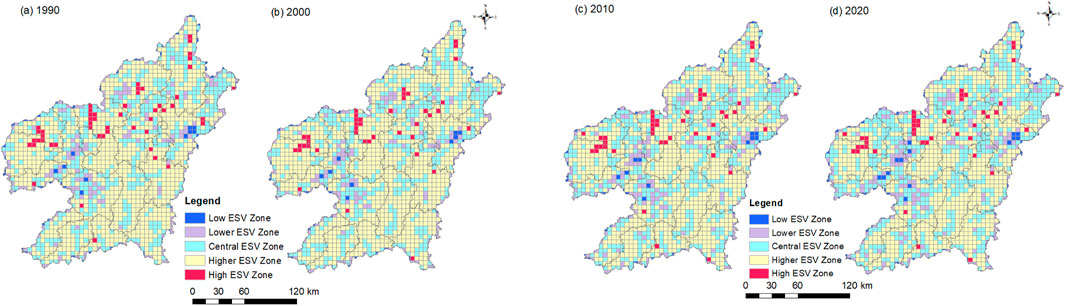
Figure 6. Spatial distribution of ESV based on grid of the GUB, 1990–2020. (a) 1990, (b) 2000, (c) 2010, (d) 2020.

Comparing the ESV levels at two different times shows that a “grade stability zone” is created if the two ESV levels are the same. The latter is referred to as a “grade up zone” if its ESV level shows improvement. Lastly, a “grade drop zone” is created if the level of the subsequent ESV declines. The results indicate that from 1990 to 2000, 95.82% of the area exhibited stable ecosystem service value (ESV) levels, while 3.42% of the area demonstrated an increase in ESV levels. Conversely, only 0.76% of the area exhibited a decrease in ESV levels, representing a very small proportion and distributed sporadically (Figure 7). From 2000 to 2010, 89.88% of the area exhibited stable ecosystem service levels, while 0.44% experienced an increase, which was minimal and distributed sporadically. Nevertheless, a decrease in levels was observed in 9.68% of the area. From 2010 to 2020, 95.66% of the area exhibited stable ESV levels, with only 0.17% demonstrating an increase, representing a minimal proportion and sporadic distribution. Conversely, a decrease in levels was observed in 4.16% of the area. From 1990 to 2020, 88.13% of the area exhibited stable ESV levels, with 0.69% demonstrating an increase. Conversely, 11.19% of the area exhibited a decline in ecosystem service levels, with the greatest concentration of affected areas observed in Dayu County, Shangyou County, Zhanggong District, and Nankang District. From a broader perspective, the proportion of areas with decreasing ESV levels of the GUB is significantly higher than those with increasing levels, indicating a risk of decline for regional ESV.

Figure 7

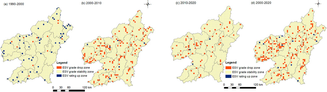
Figure 7. Temporal evolution of ESV grade of the GUB, 1990–2000, 2000–2010, 2010–2020 and 1990–2020. (a) 1990-2000, (b) 2000-2010, (c) 2010-2020, (d) 2000-2020.

3.4 Spatial variation of ESV based on administrative scale

This study selects 18 counties or districts of the GUB as the subjects of analysis, and the differences in ESV among districts/counties are presented in Table 6. During study period, the ESV of Shangyou and Ganxian exhibited an increase of 0.21% and 0.67%, respectively, while the ESV in the remaining 16 counties or districts demonstrated a decline. Zhanggong exhibited the most significant decline, at 8.44%, with Nankang, Dayu, Longnan, and Dingnan also demonstrating declines exceeding 1%.

Table 6

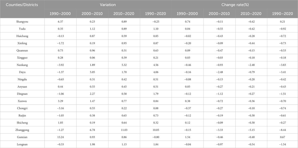
Table 6. Variation and change rate of ESV based on county scale of the GUB, 1990–2020.

To analyse regional variability using relative change rates (R), it was observed that from 1990 to 2000, the ESV of the GUB increased by 0.12%. The R values for three counties (Ganxian, Shangyou, Xunwu) exceeded 1, indicating that their ESV increased at a rate greater than that observed for the GUB as a whole. From 2000 to 2010, the ESV of the GUB exhibited a decrease of 0.49%. R values larger than 0 were shown in all 18 counties, suggesting that the ESV changes there were consistent with the general trend of the GUB. From 2010 to 2020, the ESV decreased by 0.47%. Once more, all counties exhibited R values greater than 0, thereby confirming the alignment of ESV changes with the overall trend.

From 1990 to 2020, the ESV of the GUB exhibited a net decline of 0.84%. The R values for Shangyou and Ganxian were less than 0, indicating an increase in these two counties, while the remaining 16 counties experienced a reduction in ESV, consistent with the findings of previous change rate analyses. It is noteworthy that six counties/districts (Zhanggong, Nankang, Dayu, Longnan, Dingnan, Yudu) exhibited R values greater than 1, indicating that these areas experienced greater ESV changes than the overall region, with similar trends.

3.5 Analysis of spatial autocorrelation of ESV

3.5.1 Analysis of global scale spatial autocorrelation

The global Moran’s I values for the years 1990, 2000, 2010, and 2020 were 0.318, 0.316, 0.315, and 0.316, respectively. This indicates a lack of variation across the four periods, as illustrated in Figure 8.

Figure 8

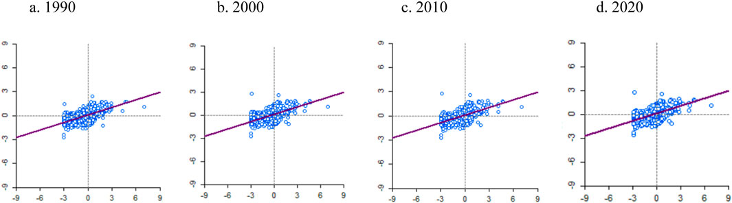
Figure 8. Spatial-temporal distribution of scatter plots of the GUB, 1990–2020. (a) 1990, (b) 2000, (c) 2010, (d) 2020.

Across the four time periods, the global Moran’s I values remained consistently positive, with significance levels below 0.01. This implies a strong positive correlation in the spatial distribution of ESV, showing that nearby grid units are highly comparable and clustered.

3.5.2 Local spatial autocorrelation analysis

The local spatial relationships between events and their neighboring events are reflected in the Local Indicators of Spatial Association (LISA) distribution map. Four categories can be used to classify these relationships: The clustering patterns are low-high, low-low, high-high, and high-low.

The results of the local spatial autocorrelation of ESV of the GUB for 1990, 2000, 2010, and 2020 show that the distribution of high-value and low-value clusters stayed rather stable, as shown in Figure 9. This shows a spatial clustering pattern and a significant positive association. The region is primarily characterised by high-high clustering and low-low clustering, with high-high clustering mainly concentrated at the boundaries of Shangyou County and Chongyi County, as well as at the intersections of Yudu County and Ruijin City, and Ganxian District and Huichang County. In contrast, low-low clustering is predominantly observed in Nankang and Zhanggong District, Xinfeng County.

Figure 9

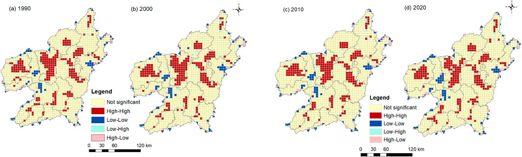
Figure 9. Spatial-temporal distribution of local spatial autocorrelation of the GUB, 1990–2020. (a) 1990, (b) 2000, (c) 2010, (d) 2020.

3.6 Exploration of drivers integrating HGB and SHAP model

To quantify the effect of each factor on ESV, the study integrated machine learning model with the SHAP analysis method. The performance of the model was evaluated based on the R², MAE and RMSE. Due to the substantial computational demands of this approach, only the data of 2020 were used to identify the driving factors of ESV.

The model evaluation metrics are delineated in Table 7, and the optimal model is identified through comprehensive analysis in terms of performance, error, and risk of overfitting. R² (Test) is a measure of the explanatory power of the model on the test set, and the closer it is to 1, the better the model performance is. The findings indicate that HGB (0.62) surpasses XGBoost (0.59), RF (0.55), GBM (0.53) and LR (0.41). Consequently, HGB emerges as the most effective model. MAE (Test) denotes the Mean Absolute Error, with smaller values being preferable. The resultant data indicates that HGB (1905.28) is outperformed by XGBoost (1965.46), RF (1978.37), GBM (2079.60) and LR (2540.72), with HGB demonstrating the lowest error rate. RMSE (Test) is the Root Mean Squared Error, and a smaller value is preferable. The findings indicate that HGB (3229.46) is outperformed by XGBoost (3351.19), followed by RF (3499.00), GBM (3555.46), and LR (3996.22), with the lowest HGB error. It is evident that HGB demonstrates superior overall performance on the test set, as evidenced by its elevated R², minimal MAE, and RMSE. The negligible discrepancy between Train (0.84) and Test (0.62) further substantiates its reduced risk of overfitting and enhanced generalisation capability. Consequently, the optimal model is identified as HGB, while the alternative model is XGBoost.

Table 7

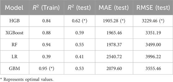
Table 7. Performance metrics of machine learning models.

The HGB plus SHAP analysis revealed the extent and direction of the effects of each environmental factor on ESV. The eight impact factors were then classified into three distinct grades, based on the results of the feature importance calculation (Figure 10). These three grades were designated as key factors, relatively important factors, and low-impact factors, respectively. Key factors are defined as those with feature importance ≥2000, Human Activity Intensity (HAI) emerged as the key factor, with a contribution value of 2285.21 (30.57%), exhibiting a substantial negative effect. That is, elevated HAI values were associated with diminished ESV predictions. The relatively important factors are those with feature importance of 500 ≤ importance value <2000, and include FVC (1681.43, 22.50%, negative effect), elevation (1038.79, 13.90%, negative effect) and SOC (851.48, 11.39%, positive effect). The low-impact factor, which is equivalent to the importance value of <500, encompasses the GDP (461.25, 6.17%, nonlinear relationship), slope (455.53, 6.09%, nonlinear relationship), temperature (362.35, 4.85%, nonlinear relationship) and precipitation (338.55, 4.53%, nonlinear relationship). Essentially, it was determined that the main parameters influencing changes in ESV were HAI, FVC, Ele, and SOC. In contrast, the contributions of economic, topographic and climatic factors were found to be comparatively negligible, though their influence should not be overlooked.

Figure 10

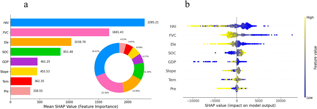
Figure 10. Detection of driving factors. (a) Bar plots of average absolute SHAP values and pie charts of contribution percentages. (b) SHAP summary plot. Note: human activity intensity (HAI), fractional vegetation cover (FVC), gross domestic product (GDP), soil organic carbon (SOC), elevation (Ele), precipitation (Pre), temperature (Tem).

The present study investigated the effects of HAI, FVC, Ele, and SOC on ESV in the study area. The findings indicated that these factors exerted substantial influence on ESV, with divergent mechanisms of action being observed. The contribution of the key characterization factors to the model predictions was quantified by SHAP feature dependency plot analysis, and the nonlinear relationships and thresholds between the features and the predictions were revealed. Figure 11 illustrates these relationships.

Figure 11

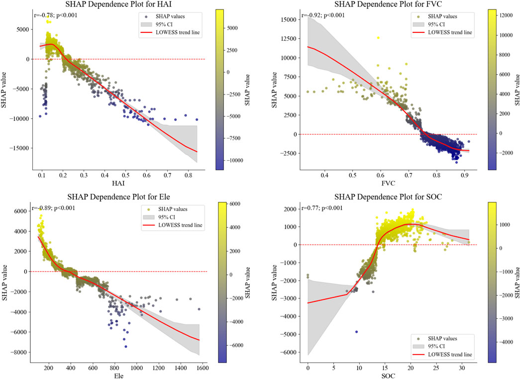
Figure 11. Partial dependency graph of key characteristic factors based on SHAP value. Note: human activity intensity (HAI), fractional vegetation cover (FVC), soil organic carbon (SOC), elevation (Ele).

A highly significant negative correlation was identified between HAI and SHAP values (r = −0.78, p < 0.001). As the HAI level increased, its effect on ESV shifted from promotion to inhibition. When HAI was less than 0.23, it exhibited a positive effect on ESV; conversely, when HAI was greater than 0.23, it demonstrated a negative effect.

A highly significant negative correlation was also identified between FVC and SHAP values (r = −0.92, p < 0.001). When FVC was less than 0.76, it exhibited a promoting effect on ESV; conversely, when FVC was greater than 0.76, the effect changed to inhibitory.

A highly significant negative correlation was also identified between altitude and SHAP values (r = −0.89, p < 0.001). At altitudes less than 400 meters, ESV exhibited a promoting effect, while at altitudes greater than 400 meters, the effect transitioned to inhibition.

A highly significant positive correlation was identified between the SHAP values and the SOC (r = 0.77, p < 0.001). When the SOC was less than 14 g/kg, it exhibited an inhibitory effect on ESV. Conversely, when the SOC was greater than 14 g/kg, the effect changed to a promoting one. The SHAP values exhibited a marked increase with rising SOC levels. However, this increase began to plateau after reaching a maximum value when the SOC level exceeded 20 g/kg.

In summary, the findings of the study demonstrated a non-linear, highly significant negative correlation between HAI, FVC, and elevation with ESV in the study area. Conversely, SOC exhibited a non-linear, highly significant positive correlation with ESV.

A thorough analysis of the uncertainty inherent in the predicted results of ESV was conducted in this study. To this end, we employed a 95% confidence interval (CI) to quantify the uncertainty. To illustrate this uncertainty, gray shading was employed to represent the 95% CI. The width of the shading is proportional to the size of the 95% CI; that is, the wider the shading, the greater the uncertainty in the prediction results.

The 95% CI of the ESV prediction result was found to be significantly larger when the HAI was greater than 0.6. This finding suggests that the ESV prediction results exhibit enhanced accuracy within the range of HAI less than 0.6. The 95% CI of the ESV prediction results was found to be significantly greater when the FVC was less than 0.6. This finding suggests that ESV predictions are more precise in cases where FVC is greater than 0.6. The 95% CI of the ESV prediction results exhibited a substantial increase when Ele was greater than 1000 meters. This finding suggests that ESV predictions exhibited higher accuracy within the range of elevation less than 1000 meters. The 95% CI of the ESV prediction results was found to be significantly greater when the SOC was less than 10 g/kg or greater than 25 g/kg. This finding indicates that ESV was more precisely predicted in the range of 10 g/kg ≤ SOC ≤25 g/kg.

In summary, the analysis of the 95% CI enabled the identification of key thresholds affecting the accuracy of the ESV prediction and the optimization of the predictive performance of the model accordingly. This finding is significant for improving the accuracy and reliability of ecosystem service value assessment.

4 Discussion

4.1 Driving mechanisms and threshold identification of ESV

In order to quantify the effect of each factor on ESV accurately, an integrated explainable machine learning approach was conducted in this study. The results indicate that HGB demonstrates superior overall performance on the test set, as evidenced by its elevated R², minimal MAE, and RMSE. The HGB model demonstrates distinct advantages over linear regression approaches by effectively capturing nonlinearity without requiring linearity assumptions. Compared to RF model, it is more computationally efficient and more adapted for analyzing huge data sets. Compared to XGBoost or GBM model, the HGB model has the benefits of seamless integration with Scikit-learn, and compatibility with sparse data (Du et al., 2025). HGB is an advanced machine learning method designed to optimize the equilibrium of efficiency, accuracy, and user-friendliness in identifying feature importance. It is an effective approach for driving factor selection (Bridge et al., 2025).

The study indicated that HAI is the key driving factor of ESV of the GUB, with a feature important of 30.57%, exhibiting a substantial negative effect of pearson analysis. SHAP-based non-linear analysis revealed that when HAI was less than 0.23, it exhibited a positive effect on ESV; conversely, when HAI was greater than 0.23, it demonstrated a negative effect. In the formula of HAI, construction land had the greatest human impact intensity coefficients among the six land use classifications. A net loss of 388.19 km²of forestland over the research period and a dramatic 105% increase in building land as a result of fast urbanization account for this decline in ESV. The rapid urbanization of GUB over the past 3 decades has resulted in a notable decline in agricultural and forestland and a notable rise in building area. The conversion of industrial structures, particularly the annual expansion of aquaculture regions, has resulted in the loss of some cropland (Chen et al., 2015; Wu et al., 2022). It is therefore evident that changes in land use of the GUB directly impact the ESV. The impact of anthropogenic activities on landscape patterns has resulted in a reduction in the ecosystem service capacity of the GUB (Qiao et al., 2025; Liu et al., 2022). This finding aligns with the results of previous studies in this field (Yao et al., 2025). The HAI is the predominant factor in ESV spatial differentiation, underscoring the repercussions of recurrent human activities on the ecological environment. The formulation of strict environmental protection policies and measures is imperative to enhance the effective management of human activities and to restrict unreasonable land use and development, thereby reducing the negative impact of human activities on the ecological environment (Hu et al., 2023).

A highly significant negative correlation was also identified between FVC and SHAP values in this study. When FVC was less than 0.76, it exhibited a promoting effect on ESV; conversely, when FVC was greater than 0.76, the effect changed to inhibitory. This finding is at odds with the conclusions of numerous preceding studies (Princelyn et al., 2025). This “abnormal” phenomenon is primarily attributable to the unique natural and socio-economic context of the GUB. A potential explanation for this phenomenon is that Ganzhou City had implemented large-scale artificial afforestation projects (primarily pure stands of cypress and pine) in rare earth tailings areas, slope farmland, and urban peripheries over the past 2 decades. These projects had led to a rapid increase in regional FVC. These artificial forests consist of a single tree species, exhibit simple community structures, and possess low understory biodiversity (Zhang et al., 2025). Consequently, the core ecological functions of carbon sequestration, water conservation, and soil retention are significantly lower than those observed in natural evergreen broadleaf forests. This phenomenon has resulted in a decline in ESV per unit area. Another potential explanation pertains to remote sensing NDVI saturation. High FVC areas (>0.7) are predominantly artificial pure forests, where NDVI has reached or approached saturation. This renders it impossible to distinguish differences in forest stand quality, thereby creating the illusion of “high FVC-low ESV” (Li Y. et al., 2025).

4.2 Assessment of ESV based on different scales

This study employs both grid-based and administrative scales to evaluate the total ESV, the unit area ESV, and their spatial distribution characteristics of the GUB. The grid method employed a 5 km × 5 km grid, representing a micro-scale approach, which facilitated the mapping of the spatial distribution of unit area ESV across the various levels within the study area. Furthermore, it permitted a comparison of the fluctuations in different levels at two distinct points in time. While micro-scale assessments can elucidate the distinctions between diverse ecological subsystems at larger scales, the outcomes obtained at smaller scales are frequently challenging to extrapolate for ecological regulation applications at broader scales (Zhang et al., 2022).

Conversely, the spatial distribution of ESV based on administrative divisions represents a macro-scale assessment, offering insights into the spatial distribution of ESV across the 18 counties or districts within the study area. By analysing relative changes, similarities and differences in the trends of each county can be identified in comparison to the overall region. Administrative scale assessments may be constrained by the influence of dominant land and ecological system components within the units, which may result in the omission of variations among subsystems. Nevertheless, the benefit of administrative scales lies in their practical applicability, enabling the collection of statistical data related to administrative units and the establishment of ecological management models, which are more straightforward to implement than grid-scale assessments (Huang et al., 2019; Yu et al., 2025). Therefore, it is advantageous to combine several scales to fully comprehend the ecological functional status of the assessment units. The study of scale characteristics in ecosystem service evaluations can be enhanced to improve the objectivity, credibility, and practicality of assessment results (Xu et al., 2019; Peng et al., 2017).

4.3 Proposes

The ESV of the GUB was evaluated, revealing an overall decline in ESV from 1990 to 2020. To improve regional ecological service value, bolster ecological security, and advance the formulation of ecological compensation policies for water supplies, the following proposals and strategies are suggested:

(1) The major purpose is to improve approach aimed at conserving and rehabilitating forest ecosystems. Prioritizing the conservation of high ESV areas is essential. Development must be rigorously limited, and the safeguarding of natural forests along with the restoration of agricultural land to forest should be strengthened to improve climate and hydrological regulatory functions, which constitute 50 percent of the ESV (Sun et al., 2025). GUB boasts a substantial forest area, and through the implementation of afforestation and grassland restoration initiatives, it has attained a notable degree of greening in the southern Jiangxi region, approaching the upper limit of the achievable greening scale. Given the sensitivity of forest land to the ESV of the region, future research should prioritize the optimization of forest stand structure and the enhancement of forest quality within mountainous forest land. This approach is expected to contribute to the continuous enhancement of the climate regulation, biodiversity maintenance, soil conservation, and landscape aesthetic ecological service values of forest land. For forest reserves, conservation should be the primary focus, with the objective of maintaining the soil and water conservation and water source protection functions of forest land (Yang et al., 2024).

(2) Careful oversight of the growth of construction land and the achievement of suitable land use patterns are crucial. Stringent regulation is essential about the unregulated expansion of construction land, especially in the 16 counties that have experienced a significant decrease in ESV. Furthermore, the execution of intense land utilization patterns is essential. Implementing ecological restoration activities in grid areas showing a reduction in ESV is essential (Zhen et al., 2021; Zhou et al., 2024).

(3) It is essential to alleviate the detrimental environmental effects resulting from HAI. It is essential to control the degree of development. The analysis reveals that HAI adversely affects ESV by 30.57%, highlighting the need to restrict high-intensity activities, such as resource development and urban expansion, in ecologically sensitive areas (Deng et al., 2025). The “high FVC-low ESV” phenomenon observed in the GUB is not attributable to the inherent harmfulness of the vegetation. Rather, it is a consequence of systemic disadvantages in terms of tree species structure, substrate quality, and site conditions that are present in high FVC areas. Subsequent measures should encompass the following: Fistly, the primary objective is to optimize the structure of artificial forests, which is to be accomplished by replanting native broad-leaved trees and enhancing community heterogeneity. Secondly, the implementation of soil improvement and functional vegetation restoration in rare earth tailings areas is imperative. Thirdly, it is imperative to differentiate between natural forests and artificial forests in statistical analyses. This is essential to circumvent potential biases that may arise from NDVI saturation.

(4) In light of the ESV clustering results, a region-specific, precision-governance strategy is hereby proposed. In the “high-high” clusters, the existing natural-forest closure policy should be maintained. Additionally, the implementation of an ecological compensation fund is imperative, along with the establishment of a maximum limit on tourism capacity. In “low-low” clusters, the following strategies should be implemented: urban renewal and brownfield remediation, rooftop greening, and sponge-city techniques to reduce impervious surface.

5 Conclusion

The principal findings are as follows:

(1) Forestland has consistently constituted the predominant terrain in the GUB, encompassing over 74% of the total area from 1990 to 2020. The ESV of the GUB showed a trend of initial expansion succeeded by a contraction, culminating in a net decrease of 21.53 × 10⁸ yuan. Regulating services constituted the predominant ecological function of the GUB, markedly exceeding other functions. Climate and hydrological regulation were first and second, respectively, accounting for roughly 50% of the overall value. (2) The grid-based examination of unit area ESV of the GUB demonstrates a notable geographical pattern, with higher values concentrated at the outside of counties or districts, and lower values found at their centers. An analysis of the ESV across administrative districts indicates that the ESV in Shangyou and Ganxian counties experienced minor rises, while the ESV in the other 16 counties showed a decrease. (3) The study identified the HGB model combined with the SHAP model as the optimal explainable machine learning model. Furthermore, the investigation into the driving factors of ESV revealed that HAI is the primary determinant of ESV of the GUB, with a feature importance of 30.57%, demonstrating a significant negative impact.

Data availability statement

The original contributions presented in the study are included in the article/Supplementary Material, further inquiries can be directed to the corresponding author.

Author contributions

XX: Methodology, Writing – original draft, Conceptualization, Writing – review and editing, Project administration. XZ: Formal Analysis, Writing – original draft. LQ: Validation, Writing – original draft. RL: Investigation, Writing – original draft.

Funding

The author(s) declare that financial support was received for the research and/or publication of this article. This study was supported by the National Natural Science Foundation of China (42261015), the Science and Technology Foundation of the Education Department of Jiangxi Province (GJJ211426).

Conflict of interest

The authors declare that the research was conducted in the absence of any commercial or financial relationships that could be construed as a potential conflict of interest.

Generative AI statement

The author(s) declare that no Generative AI was used in the creation of this manuscript.

Publisher’s note

All claims expressed in this article are solely those of the authors and do not necessarily represent those of their affiliated organizations, or those of the publisher, the editors and the reviewers. Any product that may be evaluated in this article, or claim that may be made by its manufacturer, is not guaranteed or endorsed by the publisher.

Supplementary material

The Supplementary Material for this article can be found online at: https://www.frontiersin.org/articles/10.3389/fbioe.2025.1610806/full#supplementary-material

References

Aas, K., Jullum, M., and Loland, A. (2021). Explaining individual predictions when features are dependent: more accurate approximations to shapley values. Artif. Intell. 298, 103502. doi:10.1016/j.artint.2021.103502

CrossRef Full Text | Google Scholar

Bridge, N., Charlène, B., El Ouaazizi, A., and Benyakhlef, M. A. (2025). A new data imputation technique for efficient used car price forecasting. Int. J. Electr. and Comput. Eng. 15, 2364–2371. doi:10.11591/ijece.v15i2.pp2364-2371

CrossRef Full Text | Google Scholar

Chen, M., Lu, Y., Ling, L., Wan, Y., Luo, Z., and Huang, H. (2015). Drivers of changes in ecosystem service values in ganjiang upstream watershed. Land Use Policy 47, 247–252. doi:10.1016/j.landusepol.2015.04.005

CrossRef Full Text | Google Scholar

Chen, T., and Guestrin, C. (2016). “XGBoost: a scalable tree boosting system,”Proc. 22nd ACM SIGKDD Int. Conf. Knowl. Discov. Data Min. 785–794. doi:10.1145/2939672.2939785

CrossRef Full Text | Google Scholar

Costanza, R., d'Arge, R., Groot, R. D., Farber, S., Grasso, M., Hannon, B., et al. (1997). The value of the world's ecosystem services and natural capital. Nature 387, 253–260. doi:10.1038/387253a0

CrossRef Full Text | Google Scholar

Dandolo, D., Masiero, C., Carletti, M., Pezze, D. D., and Susto, G. A. (2023). AcME-Accelerated model-agnostic explanations: fast whitening of the machine-learning Black box. Expert Syst. Appl. 214, 119115. doi:10.1016/j.eswa.2022.119115

CrossRef Full Text | Google Scholar

Deng, F., Zhu, S., Guo, J., and Sun, X. (2025). Exploring the quality of ecosystem services and the segmental impact of influencing factors in resource-based cities. J. Environ. Manag. 375, 124411. doi:10.1016/j.jenvman.2025.124411

PubMed Abstract | CrossRef Full Text | Google Scholar

Du, P., Huai, H., Wu, X., Wang, H., Liu, W., and Tang, X. (2025). Using XGBoost-SHAP for understanding the ecosystem services trade-off effects and driving mechanisms in ecologically fragile areas. Front. Plant Sci. 16, 1552818. doi:10.3389/fpls.2025.1552818

PubMed Abstract | CrossRef Full Text | Google Scholar

Feng, Y., Zhu, J., Zeng, L., and Xiao, W. (2021). Prediction of profit and loss of county-scale ecosystem service values under land use change: a case study of banan district, chongqing. Acta Ecol. Sin. 41, 3381–3393. doi:10.5846/stxb202005161250

CrossRef Full Text | Google Scholar

Gao, X., Shen, J., He, W., Zhao, X., Li, Z., Hu, W., et al. (2021). Spatial-temporal analysis of ecosystem services value and research on ecological compensation in taihu Lake basin of Jiangsu Province in China from 2005 to 2018. J. Clean. Prod. 317, 128241. doi:10.1016/j.jclepro.2021.128241

CrossRef Full Text | Google Scholar

Hu, J., Qiu, S., Luo, N., Qing, G., and Huang, C. (2023). Multi-dimensional spatial and temporal variations of ecosystem service values in the li river basin, 1990-2020. Remote Sens. 15, 2996. doi:10.3390/rs15122996

CrossRef Full Text | Google Scholar

Huang, M., Yue, W., Fang, B., and Feng, S. (2019). Scale response characteristics and geographic exploration mechanism of spatial differentiation of ecosystem service values in dabie Mountain area, central China from 1970 to 2015. Acta Geogr. Sin. 74, 1904–1920. doi:10.11821/dlxb201909015

CrossRef Full Text | Google Scholar

Huang, X., Liu, X., Jin, Y., Gao, X., and Chen, Y. (2025). Identification and attribution analysis of integrated ecological zones based on the XGBoost-SHAP model: a case study of chengdu, China. Ecol. Indic. 177, 113787. doi:10.1016/j.ecolind.2025.113787

CrossRef Full Text | Google Scholar

Jin, S., Xiao, W., Yang, S., and Zhao, D. (2020). Land use change and its ecosystem response in the yangtze river economic belt. Econ. Geogr. 40, 166–173. doi:10.15957/j.cnki.jjdl.2020.07.019

CrossRef Full Text | Google Scholar

Ke, G., Meng, Q., Finley, T., Wang, T., Chen, W., Ma, W., et al. (2017). “Light GBM: a highly efficient gradient boosting decision tree,” in Proceedings of the 31st International Conference on Neural Information Processing Systems, 3149–3157.

Google Scholar

Lee, C. Y., Hasegawa, H., and Gao, S. C. (2022). Complex-valued neural networks: a comprehensive survey. IEEE/CAA J. Autom. Sin. 9, 1406–1426. doi:10.1109/JAS.2022.105743

CrossRef Full Text | Google Scholar

Li, B., Chen, N., Wang, Y., and Wang, W. (2018). Spatio-temporal quantification of the trade-offs and synergies among ecosystem services based on grid-cells: a case study of guanzhong basin, NW China. Ecol. Indic. 94, 246–253. doi:10.1016/j.ecolind.2018.06.069

CrossRef Full Text | Google Scholar

Li, M., Yin, L., Zhang, Y., Su, X., Liu, G., Wang, X., et al. (2021). Spatio-temporal dynamics of fractional vegetation coverage based on MODIS-EVI and its driving factors in southwest China. Acta Ecol. Sin. 41, 1138–1147. doi:10.5846/stxb201907101451

CrossRef Full Text | Google Scholar

Li, W., Chen, X., Zheng, J., Zhang, F., Yan, Y., Hai, W., et al. (2025a). Effectiveness and driving mechanisms of ecological conservation and restoration in Sichuan Province, China. Ecol. Indic. 172, 113238. doi:10.1016/j.ecolind.2025.113238

CrossRef Full Text | Google Scholar

Li, W., Jing, W., Tian, Y., and Deng, N. (2025b). Prediction and trade-off analysis of forest ecological service in Hunan Province on explainable deep learning. Forests 16, 604. doi:10.3390/f16040604

CrossRef Full Text | Google Scholar

Li, Y., Liu, J., Bai, X., Feng, X., and Qiu, L. (2025c). Multi-scale spatial differentiation of ecosystem service values of the important water conservation area in the upper reaches of the yangtze river: patterns, processes and driving forces. Acta Ecol. Sin. 45, 3062–3078. doi:10.20103/j.stxb.202407311810

CrossRef Full Text | Google Scholar

Ling, F., Luo, J., Li, Y., Tang, T., Bai, L., Ouyang, W., et al. (2022). Multi-task machine learning improves multi-seasonal prediction of the Indian Ocean dipole. Nat. Commun. 13, 7681. doi:10.1038/s41467-022-35412-0

PubMed Abstract | CrossRef Full Text | Google Scholar

Liu, G., Zhang, L., and Zhang, Q. (2014b). Spatial and temporal dynamics of land use and its influence on ecosystem service value in yangtze river Delta. Acta Ecol. Sin. 34, 3311–3319. doi:10.5846/stxb201306121679

CrossRef Full Text | Google Scholar

Liu, J., Kuang, W., Zhang, Z., Xu, X., Qin, Y., Ning, J., et al. (2014a). Spatiotemporal characteristics, patterns and causes of land use changes in China since the late 1980s. J. Geogr. Sci. 24, 195–210. doi:10.1007/s11442-014-1082-6

CrossRef Full Text | Google Scholar

Liu, S., Liao, Q., Xiao, M., Zhao, D., and Huang, C. (2022). Spatial and temporal variations of habitat quality and its response of landscape dynamic in the three gorges reservoir area, China. Int. J. Environ. Res. Public Health 19, 3594. doi:10.3390/ijerph19063594

PubMed Abstract | CrossRef Full Text | Google Scholar

Liu, Z., Wu, R., Chen, Y., Fang, C., and Wang, S. (2021). Factors of ecosystem service values in a fast-developing region in China: insights from the joint impacts of human activities and natural conditions. J. Clean. Prod. 297, 126588. doi:10.1016/j.jclepro.2021.126588

CrossRef Full Text | Google Scholar

Lu, Y., Xu, C., and Wang, X. (2025). A novel modification framework for evaluating ecosystem service value in China’s five major freshwater Lakes and their surrounding cities from 2002 to 2022. Ecol. Indic. 177, 113711. doi:10.1016/j.ecolind.2025.113711

CrossRef Full Text | Google Scholar

Ouyang, Z., Wang, R., and Zhao, J. (1999). Ecosystem services and their economic valuation. Chines journal of applied ecology. 10, 635–640. doi:10.3321/j.issn:1001-9332.1999.05.034

CrossRef Full Text | Google Scholar

Pearson, D. M. (2002). The application of local measures of spatial autocorrelation for describing pattern in north Australian landscapes. J. Environ. Manag. 64, 85–95. doi:10.1006/jema.2001.0523

PubMed Abstract | CrossRef Full Text | Google Scholar

Peng, J., Hu, X., Zhao, M., Liu, Y., and Tian, L. (2017). Research progress on ecosystem service trade-offs: from cognition to decision-making. Acta Geogr. Sin. 72, 960–973. doi:10.11821/dlxb201706002

CrossRef Full Text | Google Scholar

Princelyn, I., Kadaverugu, R., and Nidheesh, P. V. (2025). Impact of open cast coal mining on ecosystem services: a case study of bhadravati mine area in central India based on three-decadal land use land cover assessment. Environ. Manag. doi:10.1007/s00267-025-02220-3

PubMed Abstract | CrossRef Full Text | Google Scholar

Qiao, B., Yang, H., Cao, X., Zhou, B., and Wang, N. (2025). Driving mechanisms and threshold identification of landscape ecological risk: a nonlinear perspective from the qilian Mountains, China. Ecol. Indic. 173, 113342. doi:10.1016/j.ecolind.2025.113342

CrossRef Full Text | Google Scholar

Shen, S., Zhu, L., Xie, Z., Fang, T., Zhao, H., and Fang, Z. (2024). Impacts of land use changes on landscape patterns and ecosystem service values in counties (villages) in ethnic regions of China: a case study of jianghua Yao autonomous county, Hunan Province. Sustainability 16, 8050. doi:10.3390/SU16188050

CrossRef Full Text | Google Scholar

Shi, J., Li, S., Song, Y., Zhou, N., Guo, K., and Bai, J. (2022). How socioeconomic factors affect ecosystem service value: evidence from China. Ecol. Indic. 145, 109589. doi:10.1016/j.ecolind.2022.109589

CrossRef Full Text | Google Scholar

Shi, Y., Wang, R., Huang, J., and Yang, W. (2012). An analysis of the spatial and temporal changes in Chinese terrestrial ecosystem service functions. Chin. Sci. Bull. 57, 2120–2131. doi:10.1007/s11434-012-4978-5

CrossRef Full Text | Google Scholar

Sothe, C., Gonsamo, A., Arabian, J., and Snider, J. (2022). Large scale mapping of soil organic carbon concentration with 3D machine learning and satellite observations. Geoderma 405, 115402. doi:10.1016/j.geoderma.2021.115402

CrossRef Full Text | Google Scholar

Sun, D., Liang, Y., and Liu, L. (2024). Impact of land use change on ecosystem service values in Guizhou province from 2000 to 2020. Resour. Environ. Yangtze Basin 33, 547–560. doi:10.11870/cjlyzyyhj202403008

CrossRef Full Text | Google Scholar

Sun, Y., Qi, M., Wang, W., Cai, J., and Tian, F. (2025). Exploration of the multi-scenario spatiotemporal evolution, trade-off and synergy relationships, and driving factors of ecosystem services in Henan Province, China, under the background of land use change. Front. Ecol. Evol. 13, 1565632. doi:10.3389/fevo.2025.1565632

CrossRef Full Text | Google Scholar

Wang, H., Qin, F., Zhu, J., and Zhang, C. (2017). The effects of land use structure and landscape pattern change on ecosystem service values. Acta Ecol. Sin. 37, 1286–1296. doi:10.5846/stxb201606291295

CrossRef Full Text | Google Scholar

Wang, S., Liu, Z., Chen, Y., and Fang, C. (2021). Factors influencing ecosystem services in the pearl river Delta, China: spatiotemporal differentiation and varying importance. Resour. Conserv. Recycl. 168, 105477. doi:10.1016/j.resconrec.2021.105477

CrossRef Full Text | Google Scholar

Wang, Y., Xue, Z., Yang, Y., Ren, W., and Ju, A. (2025). The impact of ecological vulnerability on ecosystem service value and threshold identification: a case study of the zhangjiakou-chengde area, China. Front. Environ. Sci. 13, 1583841. doi:10.3389/fenvs.2025.1583841

CrossRef Full Text | Google Scholar

Wang, Y., Zhang, Z., and Chen, X. (2024). Impact of land use change on water-related ecosystem services under multiple ecological restoration scenarios in the ganjiang river basin, China. Forests 15, 1225. doi:10.3390/f15071225

CrossRef Full Text | Google Scholar

Wei, X., Xin, S., Zhang, Y., Long, Y., and Zhang, X. (2023). Spatial difference of ecological services and its influencing factors under different scales: taking the nanchang urban agglomeration as an example. Acta Ecol. Sin. 43, 7585–7597. doi:10.20103/j.stxb.202203310811

CrossRef Full Text | Google Scholar

Wu, Z., Du, S., Huang, Y., Zheng, B., Xie, Z., Luo, C., et al. (2022). Assessment of ecological conservation effect in southern Jiangxi province based on gross ecosystem product. Acta Ecol. Sin. 42, 6670–6683. doi:10.5846/stxb202104181007

CrossRef Full Text | Google Scholar

Xiao, J., Qiao, B., Chen, G., Shi, F., Cao, X., and Zhu, C. (2020). Land use change and evolution of ecosystem service value in maduo county of source region of the yellow river. Acta Ecol. Sin. 40, 510–521. doi:10.5846/stxb201902250346

CrossRef Full Text | Google Scholar

Xie, G., Lu, C., Leng, Y., Zheng, D., and Li, S. (2003). Ecological assets valuation of the Tibetan Plateau. J. Nat. Resour. 18, 189–196. doi:10.3321/j.issn:1000-3037.2003.02.010

CrossRef Full Text | Google Scholar

Xie, G., Zhang, C., Zhang, L., Chen, W., and Li, S. (2015). Improvement of the evaluation method for ecosystem service value based on per unit area. J. Nat. Resour. 30, 1243–1254. doi:10.11849/zrzyxb.2015.08.001

CrossRef Full Text | Google Scholar

Xiong, K., Zhang, N., Kung, C., and Kong, F. (2019). Determinants of residents’ willingness to accept and their levels for ecological conservation in ganjiang river basin, China: an empirical analysis of survey data for 677 households. Sustainablility 11, 6138. doi:10.3390/su11216138

CrossRef Full Text | Google Scholar

Xu, N., Sun, S., Xue, D., and Guo, L. (2019). Ecosystem service value and its spatial response to human interference on the basis of terrain gradient in gannan region, China. Acta Ecol. Sin. 39, 97–107. doi:10.5846/stxb201809121965

CrossRef Full Text | Google Scholar

Xu, X. (2025). Construction of ecological security patterns in hilly cities based on morphological spatial pattern analysis and minimum cumulative resistance models: a case study of ganzhou, China. Appl. Ecol. Environ. Res. 23, 1475–1496. doi:10.15666/aeer/2301_14751496

CrossRef Full Text | Google Scholar

Yan, E., Lin, H., Wang, G., and Xia, C. (2014). Analysis of evolution and driving force of ecosystem service values in the three gorges reservoir region during 1990-2011. Acta Ecol. Sin. 34, 5962–5973. doi:10.5846/stxb201312263032

CrossRef Full Text | Google Scholar

Yang, G., Lü, K., and Li, F. (2022). Spatial and temporal correlation analysis of land use change and ecosystem service value in nanchang city based on grid scale. China Land Sci. 36, 121–130. doi:10.11994/zgtdkx.20220808.090340

CrossRef Full Text | Google Scholar

Yang, J., Deng, W., Zhang, G., and Cui, X. (2024). Linking endangered species protection to construct and optimize ecological security patterns in the national ecological civilization construction demonstration zone: a case study of yichang, China. Ecol. Indic. 158, 111579. doi:10.1016/j.ecolind.2024.111579

CrossRef Full Text | Google Scholar

Yang, X., Luo, Z., and Luo, S. (2025a). Multi-scenario ecosystem risk identification and early warning coupling 'pattern-service-stability': a case study of the Poyang Lake plain, China. Environ. Res. Lett. 20, 084030. doi:10.1088/1748-9326/ade72f

CrossRef Full Text | Google Scholar

Yang, Y., Qin, Y., and Yuan, Z. (2025b). Improving sustainable land use level with the aim of enhancing urban ecosystem service value: a case study of Xi'an in China. Environ. Monit. Assess. 197, 267. doi:10.1007/s10661-025-13709-z

PubMed Abstract | CrossRef Full Text | Google Scholar

Yao, X., Zeng, J., and Li, W. (2015). Spatial correlation characteristics of urbanization and land ecosystem service value in wuhan urban agglomeration. Trans. Chin. Soc. Agric. Eng. 31, 249–256. doi:10.11975/j.issn.1002-6819.2015.09.038

CrossRef Full Text | Google Scholar

Yao, Z., Chen, S., and Huang, Y. (2025). Exploring the threshold of human activity impact on urban ecosystem service value: a case study of hefei, China. Sci. Rep. 15, 24118. doi:10.1038/s41598-025-09877-0

PubMed Abstract | CrossRef Full Text | Google Scholar

Ye, Q., Liu, G., Tian, G., Ye, J., Chen, S., Huang, C., et al. (2004). Analysis of spatiotemporal composite changes in land use in the yellow river Delta. Sci. China, Ser. D, Earth Sci. 34, 461–474. doi:10.3969/j.issn.1674-7240.2004.05.009

CrossRef Full Text | Google Scholar

Yu, T., Huang, X., Chen, X., Liang, J., Li, X., and Cui, X. (2025). Deciphering the spatial code of the yellow river basin: a novel framework for optimizing land use functions and zoning identification strategies. J. Environ. Manag. 389, 126168. doi:10.1016/j.jenvman.2025.126168

PubMed Abstract | CrossRef Full Text | Google Scholar

Zhang, B., Li, Z., Feng, Q., Lu, Z., Zhang, B., and Cheng, W. (2024). Evolution of ecosystem service values in qilian Mountains based on land-use change from 1990 to 2020. Acta Ecol. Sin. 44, 4187–4202. doi:10.20103/j.stxb.202211023130

CrossRef Full Text | Google Scholar

Zhang, J., Yang, W., Li, J., Shen, S., Ma, L., and Chen, L. (2025). Spatio-temporal variation and driving factors of ecosystem services value in beijing. Acta Ecol. Sin. 45, 306–318. doi:10.20103/j.stxb.202312312885

CrossRef Full Text | Google Scholar

Zhang, L., and Fu, B. T. (2014). he progress in ecosystem services mapping: a review. Acta Ecol. Sin. 34, 316–325. doi:10.5846/stxb201303110391

CrossRef Full Text | Google Scholar

Zhang, M., Shi, W., and Xu, Z. (2020). Systematic comparison of five machine-learning models in classification and interpolation of soil particle size fractions using different transformed data. Hydrol. Earth Syst. Sci. 24, 2505–2526. doi:10.5194/hess-24-2505-2020

CrossRef Full Text | Google Scholar

Zhang, X., Zheng, Z., Sun, S., Wen, Y., and Chen, H. (2023). Study on the driving factors of ecosystem service value under the dual influence of natural environment and human activities. J. Clean. Prod. 420, 138408. doi:10.1016/j.jclepro.2023.138408

CrossRef Full Text | Google Scholar

Zhang, Y., Wang, Y., Jin, Z., Zhuo, S., and Li, J. (2021). Review of high-quality economic development under the constraint of ecological security. Ecol. Econ. 37, 182–190.

Google Scholar

Zhang, Z., Nie, T., Gao, Y., Sun, S., and Gao, J. (2022). Study on temporal and spatial characteristics of coupling coordination correlation between ecosystem services and economic-social development in the yangtze river economic belt. Resour. Environ. Yangtze Basin 31, 1086–1099. doi:10.11870/cjlyzyyhj202205013

CrossRef Full Text | Google Scholar

Zhao, Y., Gao, G., Ding, G., Wang, L., Chen, Y., Zhao, Y., et al. (2022). Assessing the influencing factors of soil susceptibility to wind erosion: a wind tunnel experiment with a machine learning and model-agnostic interpretation approach. Catena 215, 106324. doi:10.1016/j.catena.2022.106324

CrossRef Full Text | Google Scholar

Zhao, Y., Luo, L., Zhang, L., Sun, J., and Lu, Z. (2025). Spatiotemporal evolution and driving forces of ecosystem service values in the yellow river Delta. Ecol. Indic. 173, 113432. doi:10.1016/j.ecolind.2025.113432

CrossRef Full Text | Google Scholar

Zhen, B., Huang, Q., Tao, L., Xie, Z., Ai, B., Zhu, Y., et al. (2021). Landscape pattern change and its impacts on the ecosystem services value in southern Jiangxi province. Acta Ecol. Sin. 41, 5940–5949. doi:10.5846/stxb202006171584

CrossRef Full Text | Google Scholar

Zhou, J., Nie, G., and Liu, Y. (2024). Multi-criteria comparison analysis of spatial equity for emergency shelters in old and new urban districts: a case study in wuhua district and chenggong district of kunming city, China. Int. J. Disaster Risk Reduct. 108, 104547. doi:10.1016/j.ijdrr.2024.104547

CrossRef Full Text | Google Scholar