A CEEMDAN-GNN-transformer hybrid model for air quality index forecasting: a case study of Chang’an town, Dongguan, China

Air pollution has emerged as a pressing global environmental issue, and accurate forecasting plays a critical role in environmental governance and public health protection. This study proposes an enhanced air quality forecasting model based on a hybrid CEEMDAN-GNN-Transformer architecture, and conducts an empirical analysis using data from Chang’an Town, Dongguan, China. The proposed model first employs Complete Ensemble Empirical Mode Decomposition with Adaptive Noise (CEEMDAN) to extract multi-scale temporal features and mitigate non-stationary noise in the data. Then, a Graph Neural Network (GNN) is applied to capture the spatial dependencies among various air pollutants. Finally, a Transformer model is utilized to model complex temporal dependencies and improve the capture of long-term trends. The research uses historical air quality monitoring data from 2015 to 2024, including concentrations of PM_2.5, PM₁₀, SO₂, CO, NO₂, and O₃ as input features, with the Air Quality Index (AQI) as the prediction target. Model performance is enhanced through ablation studies and hyperparameter tuning, and is compared against several mainstream baseline models. Experimental results demonstrate that the proposed CEEMDAN-GNN-Transformer model outperforms traditional approaches in terms of MAE, MSE, and R² metrics, achieving superior prediction accuracy and robustness. This study not only contributes to the theoretical advancement of air quality forecasting methodologies but also provides a more precise predictive tool for environmental management and public health risk prevention, offering significant practical value.

1 Introduction

Air pollution has emerged as one of the most pressing environmental issues worldwide, significantly impacting human health, ecosystems, and economic development. According to the World Health Organization (WHO), over seven million premature deaths annually are attributed to diseases related to air pollution. The United Nations Environment Programme (UNEP) further emphasizes its multifaceted consequences, ranging from respiratory and cardiovascular disorders to ecological degradation and climate change. Key air pollutants—such as fine particulate matter (PM_2.5, PM₁₀), sulfur dioxide (SO₂), carbon monoxide (CO), nitrogen dioxide (NO₂), and ozone (O₃)—jointly determine the Air Quality Index (AQI), a composite metric widely used to assess atmospheric pollution levels and associated health risks (Horn and Dasgupta, 2024).

Although the Chinese government has implemented a series of policies to strengthen air pollution control, such as the Air Pollution Prevention and Control Action Plan, the Three-Year Action Plan to Win the Blue Sky Defense Battle, and the Air Quality Improvement Action Plan, the overall air quality in China has improved in recent years. However, some rapidly industrializing and urbanizing regions still face severe air pollution problems. According to the 2023 Bulletin on China’s Ecological and Environmental Status issued by the Ministry of Ecology and Environment, 121 out of 337 cities at the prefecture-level or above still fail to meet the air quality standards. While the PM_2.5 concentration in the Pearl River Delta region has decreased by 34% compared to 2015, the number of days with ozone (O₃) exceeding the standard has increased to 12.7%, making it the primary pollutant.

Chang’an Town in Dongguan, a typical industrial town in the Pearl River Delta, continues to experience significant air quality issues due to the dual pressures of industrial clustering and high population density. In 2022, the annual average PM_2.5 concentration in Chang’an Town was 32 μg/m³, which is below the national secondary standard (35 μg/m³) but still significantly higher than the World Health Organization’s recommended standard (5 μg/m³). Additionally, the proportion of days with good air quality was lower than the average for Dongguan (Guangdong Provincial Department of Ecology and Environment, 2023). Against the backdrop of high population density and intense industrial emissions, developing air quality forecasting models with high accuracy and strong generalization ability is of great practical significance for pollution control and environmental governance decision-making.

High-accuracy forecasting models can provide at least a 72-h warning window for pollution events, which is crucial for environmental governance, public health protection, and policy formulation. The variation in air quality is influenced by multiple factors, exhibiting high non-linearity, non-stationarity, and spatial correlation. Traditional statistical models and some machine learning methods often struggle to simultaneously capture multi-scale features, spatial dependencies, and long-term temporal relationships in complex air quality time series data (Mishra and Gupta, 2024). With the rapid development of deep learning and time series modeling, forecasting methods based on advanced models such as Transformer and Graph Neural Networks (GNN) have demonstrated superior performance. However, single deep learning models often fail to adequately capture the spatiotemporal relationships and multi-scale characteristics between pollutants, which can hinder prediction accuracy. Therefore, combining and optimizing different models has become a key research direction for improving air quality prediction accuracy. Furthermore, due to the presence of significant noise and complex periodic features in air pollution data, employing signal decomposition methods can effectively separate the time series of pollutants, improving the stability and generalization ability of the forecasting model (Agbehadji and Obagbuwa, 2024).

To address these challenges, this paper proposes a hybrid air quality forecasting framework based on Complete Ensemble Empirical Mode Decomposition with Adaptive Noise (CEEMDAN), GNN, and Transformer. The framework first applies CEEMDAN to decompose the raw pollutant time series data, reducing noise interference and extracting the primary trend information. Next, GNN is used to model the complex spatiotemporal dependencies among pollutants. Finally, the Transformer model is employed to achieve precise forecasting of AQI by leveraging its strong representation power. This study focuses on Chang’an Town, Dongguan, using air pollution data from 2015 to 2024, with pollutants such as PM_2.5, PM₁₀, SO₂, CO, NO₂, and O₃ as input features, and AQI as the target variable. Empirical analysis is conducted to validate the effectiveness and superiority of the proposed model.

The main contributions of this study are as follows: A hybrid deep learning architecture integrating CEEMDAN, GNN, and Transformer. This model effectively captures the multi-scale, nonlinear, and spatiotemporal characteristics inherent in air quality time series data. The model is empirically validated using a decade-long dataset of air pollutant concentrations collected from an industrial town with complex environmental conditions, demonstrating its robustness in real-world scenarios. The experimental results show that the proposed framework significantly outperforms baseline models in terms of Mean Absolute Error (MAE), Mean Squared Error (MSE), and the coefficient of determination (R²), thereby confirming its superior predictive accuracy.

The remainder of this paper is structured as follows: Section 2 presents a literature review. Section 3 introduces the model architecture and methodology in detail. Section 4 discusses data collection and feature processing. Section 5 presents the experimental design and result analysis. Section 6 concludes the study and outlines future research directions.

2 Literature review

In recent years, with the rapid advancement of data science and artificial intelligence, numerous novel forecasting methodologies have emerged, including deep learning models, GNN, and Transformer-based architectures. These approaches have shown considerable potential in air quality forecasting. This section provides a comprehensive review of prior studies on air quality prediction, with a particular focus on hybrid models that integrate CEEMDAN, GNN, and Transformer techniques.

Air quality forecasting, as a crucial task in environmental science, aims to predict future air quality conditions by considering various influencing factors such as meteorology, traffic, industrial emissions, and socioeconomic activities (Abirami and Chitra, 2021). Traditional forecasting approaches predominantly rely on statistical models such as Autoregressive Integrated Moving Average (ARIMA) and Seasonal ARIMA (SARIMA). These methods perform reasonably well under stationary conditions. For example, Sharma et al. (2025) applied ARIMA to predict PM_2.5 concentrations in satellite cities around Delhi, India, demonstrating that while ARIMA can capture temporal trends in stationary series, it struggles with external influencing factors and nonlinearities in the data.

To address these limitations, machine learning and deep learning models have been increasingly adopted. Techniques such as Support Vector Machines (SVM), Random Forests (RF), Adaptive Boosting (AdaBoost), and Extreme Gradient Boosting (XGBoost) have improved predictive performance, yet often fail to fully capture spatiotemporal dependencies in the data (Zaini et al., 2022). Wang et al. (2023), for instance, used XGBoost to improve PM_2.5 predictions, though the model was limited in its ability to model spatial correlations. Similarly, K-Nearest Neighbors (KNN) and Gradient Boosted Decision Trees (GBDT) have shown flexibility and adaptability for short-term prediction tasks, but encounter challenges when handling long-term or spatially coupled data (Liu et al., 2021).

In the deep learning domain, Long Short-Term Memory (LSTM), Convolutional Neural Networks (CNN), and Gated Recurrent Unit (GRU) models have been widely applied to tasks like air quality prediction, where they excel in modeling long-term sequential data. LSTM and GRU are particularly adept at capturing temporal dependencies, though they often require large amounts of training data and computational resources due to their high complexity (Li et al., 2022). Kumbalaparambi et al. (2023) proposed a BiLSTM prediction model that effectively captures time dependencies, though the model’s interpretability is weak. CNN, known for its powerful feature extraction ability, has also been widely applied to air quality prediction, especially when dealing with spatial information or extracting local temporal features. Some studies have attempted to combine CNN with Transformer models, using CNN to extract local pattern features and Transformer to model long-range dependencies, thus balancing short-term feature capture with long-term trend modeling (Chen et al., 2022).

Empirical Mode Decomposition (EMD) and its improved version, Complete Ensemble Empirical Mode Decomposition with Adaptive Noise (CEEMDAN), have been widely used in time series data denoising and signal decomposition. CEEMDAN decomposes complex time series signals into multiple intrinsic mode functions (IMFs), each representing a component of the data in a specific frequency band, effectively removing noise while preserving the key features of the signal (Ameri et al., 2023). CEEMDAN has been applied primarily in the data preprocessing stage of air quality prediction by decomposing different frequency components to optimize the model inputs and enhance prediction accuracy. Wu et al. (2024) utilized CEEMDAN to decompose PM_2.5 sequences in air quality prediction, successfully removing high-frequency noise and improving model stability. Studies have shown that combining CEEMDAN with deep learning models such as LSTM and GRU can effectively remove noise and short-term fluctuations, thereby enhancing the model’s ability to capture long-term trends and improving prediction accuracy (Wu et al., 2022). Zhang et al. (2023) proposed a CEEMDAN-LSTM hybrid model for air quality prediction, demonstrating the effectiveness of this approach in noise reduction and improving model accuracy.

The spatiotemporal distribution characteristics of air quality pose challenges for traditional time series models in handling spatial dependencies. Graph Neural Networks (GNN) have been widely applied in air quality prediction due to their ability to capture spatial dependencies by constructing graph structures and learning relationships between nodes. GNN models in air quality prediction typically model the propagation and diffusion of pollutants based on the spatial correlations between monitoring stations (Chen et al., 2023). Ge et al. (2021) employed Graph Convolutional Networks (GCN) for urban air quality prediction, successfully incorporating the spatial correlations between monitoring stations to improve prediction accuracy. GNN can learn the diffusion paths of pollutants across different regions, providing more accurate spatial predictions.

The Transformer model, proposed in 2017, has made significant breakthroughs in various fields due to its self-attention mechanism, which effectively handles dependencies in long-time series data. Unlike traditional Recurrent Neural Networks (RNN) and LSTM models, Transformer does not rely on sequential processing and can compute in parallel, significantly improving computational efficiency (Zhang and Zhang, 2023). In air quality prediction, Transformer and its variants (e.g., Informer, Longformer) have shown their ability to capture complex dependencies in long-time series through self-attention mechanisms. Liang et al. (2023) proposed a Transformer-based time series prediction model specifically for handling long-term dependencies in multivariate time series data, achieving good predictive performance. Transformer models, by processing large amounts of historical data, are able to better capture the long-term trends in air quality variations, supporting long-term air quality forecasting. He et al. (2025) proposed a Transformer-based air pollution prediction model that leverages the self-attention mechanism to enhance long-term time dependency modeling.

Hybrid models that combine multiple methods have demonstrated improved performance by leveraging the strengths of different algorithms. CEEMDAN can be integrated with deep learning models like LSTM and GRU to first perform noise reduction and signal decomposition, followed by temporal modeling, thereby enhancing both robustness and accuracy. Tang et al. (2024) proposed a CEEMDAN-SE-GRU model for air quality forecasting, which effectively captured AQI variations by addressing noise and nonlinear components. Models combining GNN and Transformers can simultaneously process temporal sequences and spatial dependencies, enabling more accurate and context-aware forecasts. For instance, Ban and Shen (2022) proposed a CEEMDAN–LSTM–BP–ARIMA hybrid model that demonstrated strong adaptability for short-term PM_2.5 prediction.

In summary, current research in air quality prediction exhibits the following trends: (1)Traditional statistical models such as ARIMA and SARIMA remain valuable for stationary, univariate prediction tasks but underperform in nonlinear, multivariate contexts; (2) Machine learning models outperform statistical methods in feature interaction modeling but struggle to jointly capture spatial dependencies and multi-scale temporal features; (3) Deep learning models each possess distinct strengths but often cannot simultaneously address multi-scale temporal structures and spatial correlations within a single architecture; (4) CEEMDAN–deep learning hybrids enhance noise reduction and trend extraction but are typically confined to single prediction frameworks, lacking integration of spatial and long-range temporal modeling; (5) GNN–Transformer integrations have been applied in other fields but remain underexplored for highly volatile industrial air pollution scenarios.

Accordingly, three major research gaps can be identified: (1) The absence of a unified framework integrating multi-scale signal decomposition, spatial dependency modeling, and long-range temporal dependency capture; (2) Limited empirical validation in typical high-pollution, highly non-stationary industrial zones, restricting the assessment of model stability and generalization; (3) Insufficient fusion between long-range temporal and spatial diffusion modeling, hindering comprehensive characterization of pollutant evolution mechanisms.

Air quality forecasting is a highly complex, multi-factor task involving the nonlinear nature of time series data, spatial dependencies, and the integration of heterogeneous data sources. Although substantial progress has been made in recent years, existing predictive models often struggle to simultaneously capture the nonlinearities, multi-scale temporal structures, and spatial correlations inherent in pollution data. This limitation becomes particularly pronounced in densely populated, heavily industrialized regions such as Chang’an Town in Dongguan, China, where pollutant emissions exhibit strong source heterogeneity, abrupt fluctuations, and pronounced spatiotemporal coupling—posing considerable challenges to conventional forecasting approaches.

To address these challenges, this study proposes a novel hybrid deep learning framework that integrates CEEMDAN, GNN, and Transformer architectures to jointly model multi-scale structures, spatial diffusion patterns, and long-term temporal dependencies in air quality data. CEEMDAN effectively handles the non-stationarity of pollution time series by decomposing them into intrinsic mode functions across multiple frequency bands, thereby enhancing noise reduction and feature representation. GNN is employed to capture the spatial propagation of pollutants among monitoring stations, uncovering complex regional diffusion relationships. Meanwhile, the Transformer model leverages self-attention mechanisms to strengthen the representation of long-range dependencies and complex temporal dynamics.

This integrated framework overcomes the limitations of single-model approaches in jointly modeling spatial and temporal features, and is particularly well-suited to real-world conditions in industrial zones like Chang’an Town, where pollutant concentrations are highly volatile and data are frequently contaminated by noise. By introducing this innovative architecture, the study offers a more adaptive and robust solution for air quality forecasting in environments characterized by strong nonlinearity and spatiotemporal heterogeneity. It provides a scientifically grounded, data-driven tool to support environmental monitoring, early warning systems, and policy-making in complex industrial settings.

3 Methods

3.1 CEEMDAN for signal decomposition

The Complete Ensemble Empirical Mode Decomposition with Adaptive Noise (CEEMDAN) is an advanced signal processing method designed for analyzing nonlinear and non-stationary time series. It extends the original Empirical Mode Decomposition (EMD) by improving the decomposition stability and mitigating mode mixing—an issue in traditional EMD where intrinsic mode functions (IMFs) with overlapping frequency content compromise the interpretability of results (Guo et al., 2023).

CEEMDAN enhances EMD by introducing Gaussian white noise into the decomposition process. Initially, Gaussian noise is added to the original signal to generate multiple noisy versions. Each noisy signal is decomposed using EMD to extract its IMFs. Subsequently, the corresponding IMFs from each realization are averaged to obtain a more robust and stable decomposition. The incorporation of adaptive noise further ensures that each IMF retains high independence and spectral purity, thereby improving decomposition accuracy. This process enables effective noise reduction while preserving the underlying characteristics of the original signal (Hu et al., 2021). In this study, the IMFs and residual components extracted via CEEMDAN serve as refined input features for subsequent spatial-temporal modeling.

3.2 GNN for spatial feature extraction

Figure 1 illustrates the basic workflow of Graph Neural Networks (GNN), whose main objective is to extract spatial features from multivariate data at each time step and model the dependencies between variables. Specifically, a graph structure is used to represent the relationships between variables:

Figure 1

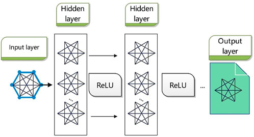
Figure 1. Graph neural network workflow.

Nodes represent the 18 variables, including AQI and major pollutant concentrations (e.g., PM_2.5, PM₁₀, SO₂, CO, NO₂, O₃_8 h), as well as the IMFs (IMF_1 to IMF_10) and Residue from CEEMDAN decomposition.

Edges define the connections between the variables through an adjacency matrix.

Graph Convolutional Networks (GCN), a common variant of GNN, are used to update the spatial features, and the update process can be represented by the following equations, as shown in Equations 1–3 (Zhou et al., 2020):

$H_t=\sigma \left(\stackrel{\sim }{A}{X}_{t}W+b\right)(1)$

Where $X_t\in {\mathbb{R}}^{N\times F}$ represents the input feature at time $\mathrm{t}$, $\stackrel{\sim }{A}\in {\mathbb{R}}^{N\times N}$ is the normalized adjacency matrix. $W\in {\mathbb{R}}^{F\times D}$ is the learnable weight matrix, where $\mathrm{D}$ is the hidden layer dimension. $b\in {\mathbb{R}}^D$ represents the bias term. $\sigma$ is the activation function, representing spatial features at time $\mathrm{t}$.

To enhance expressiveness, multiple layers can be stacked, allowing the network to capture more complex relationships.

$H_t^{\left(l\right)}=\sigma \left(\stackrel{\sim }{A}{H}_t^{\left(l-1\right)}{W}^{\left(l\right)}+b^{\left(l\right)}\right)(2)$

$H_t^{\left(l\right)}=X_t$ is the initial input, and $H_t^{\left(l\right)}$ is the output of the $L$ th layer, serving as the final spatial feature. The GNN is applied across all time steps, producing the output as:

$H=\left[H_1,H_2,\dots ,H_T\right]\in {\mathbb{R}}^{T\times N\times F}(3)$

This process is applied at every time step, yielding spatial features across time.

3.3 Feature fusion mechanism

The spatial features extracted by GNN need to be fused with the original input features to generate a unified input for the Transformer model.

To fully leverage the spatial feature extraction capabilities of GNN, the spatial features are fused with the original input features to form a combined feature suitable for Transformer modeling. The fusion process is carried out as shown in Equations 4–6:

Concatenation: The features are concatenated.

$Z_t=\left[X_t,H_t\right]\in {\mathbb{R}}^{N\times \left(F+D\right)}(4)$

Linear Transformation: A linear transformation is applied.

$Zt=W_f\left[X_t,H_t\right]+b_f(5)$

Attention Fusion: Multi-head attention mechanisms dynamically fuse the features.

$Z_t=MultiHeadAttention\left(Q=X_t,K=H_t,V=H_t\right)(6)$

Where $Q$ (queries) are derived from original features, and $K$ ((keys) and $V$ (values) are obtained from GNN features. The output $Z_t\in {\mathbb{R}}^{N\times D^{`}}$ is reshaped into $\mathrm{Z}\in {\mathbb{R}}^{\mathrm{T}\times \mathrm{N}\times {\mathrm{D}}^{`}}$, facilitating dynamic weighted fusion and improving sensitivity to key variables.

3.4 Transformer for temporal modeling

Figure 2 illustrates the main structure of the Transformer model. The Transformer model receives the fused feature $\mathrm{Z}$, which is used to model the temporal dependencies in the time series for future prediction. The input processing first reshapes $\mathrm{Z}$ to match the input format required by the Transformer. Then, position encoding is applied to add temporal information to the input sequence, as Transformer models do not inherently account for sequence order (Vaswani et al., 2017). Position encoding typically uses sinusoidal functions, as shown in Equations 7, 8:

${\text{PE}}_{\left(\mathrm{t},2\mathrm{i}\right)}=\mathrm{s}\text{in}\left(\frac{\mathrm{t}}{{1000}^{\frac{2\mathrm{i}}{{\mathrm{d}}_{\text{model}}}}}\right)(7)$

${\text{PE}}_{\left(\mathrm{t},2\mathrm{i}+1\right)}=\cos \left(\frac{\mathrm{t}}{{1000}^{\frac{2\mathrm{i}}{{\mathrm{d}}_{\text{model}}}}}\right)(8)$

Figure 2

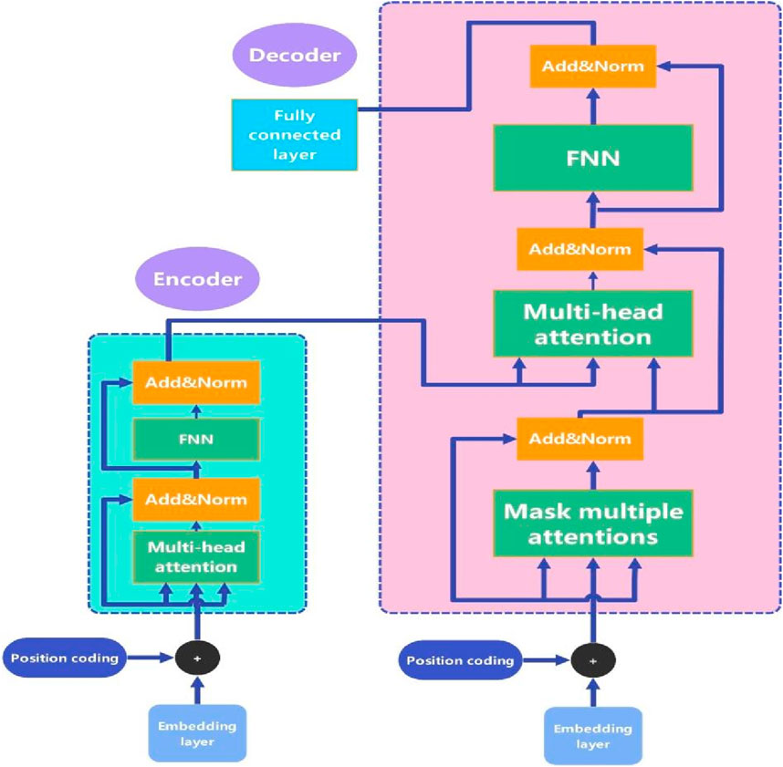
Figure 2. Architecture of the transformer model.

In the attention mechanism, the input sequence is projected into queries ($\mathrm{Q}$), keys ($\mathrm{K}$), and values ($\mathrm{V}$), where ${\mathrm{W}}_{\mathrm{Q}}$, ${\mathrm{W}}_{\mathrm{K}}$ , and ${\mathrm{W}}_{\mathrm{V}}$ are trainable projection matrices. The attention score is computed by taking the dot product of the query and key, followed by scaling and applying the Softmax function, as shown in Equation 9:

$\text{Attention}\left(\mathrm{Q},\mathrm{K},\mathrm{V}\right)=\text{Softmax}\left(\frac{\mathrm{Q}·{\mathrm{K}}^{\mathrm{t}}}{\sqrt{{\mathrm{d}}_{\mathrm{k}}}}\right)·\mathrm{V}(9)$

Multi-head attention involves parallelizing multiple self-attention heads to capture different feature subspaces. For each head $\mathrm{h}$, the computation can be represented as shown in Equation 10:

${\mathrm{h}\text{ead}}_{\mathrm{h}}=\text{Attention}\left({\mathrm{Q}}_{\mathrm{h}},{\mathrm{K}}_{\mathrm{h}},{\mathrm{V}}_{\mathrm{h}}\right)(10)$

The outputs of all heads are concatenated and passed through a linear transformation, as shown in Equation 11:

$\text{MultiHead}\left(\mathrm{Q},\mathrm{K},\mathrm{V}\right)=\text{Concat}\left({\mathrm{h}\text{ead}}_1,\dots ,{\mathrm{h}\text{ead}}_{\mathrm{h}}\right)·{\mathrm{W}}_{\mathrm{O}}(11)$

The attention output is then passed through a Feed-Forward Network (FFN) consisting of two linear layers with a ReLU activation, as shown in Equation 12:

$\text{FFN}\left(\mathrm{x}\right)=\max \left(0,\mathrm{x}·{\mathrm{W}}_1+{\mathrm{b}}_1\right)·{\mathrm{W}}_2+{\mathrm{b}}_2(12)$

Residual connections and Layer Normalization are used after each sub-layer to ensure training stability, as shown in Equation 13:

$\text{LayerNorm}\left(\mathrm{x}+\text{SubLayer}\left(\mathrm{x}\right)\right)(13)$

For time series forecasting, the output of the final Transformer layer is typically the predicted sequence, representing future values at each time step. If ${\mathrm{Z}}_{\text{out}}$ is the output of the final Transformer layer, it can be mapped to the desired prediction dimensions through a linear layer, as shown in Equation 14:

$\widehat{\mathrm{y}}={\mathrm{Z}}_{\text{out}}·{\mathrm{W}}_{\mathrm{y}}+{\mathrm{b}}_{\mathrm{y}}(14)$

3.5 Overall model workflow and design logic

Figure 3 presents the overall architecture of the proposed CEEMDAN-GNN-Transformer hybrid framework. The process begins with data collection and preprocessing. The target air quality variable (AQI) is decomposed using CEEMDAN into IMFs and a residual component to reduce non-stationarity and noise.

Figure 3

Figure 3. Overall technical framework of the proposed model.

An ablation study is conducted to verify the effectiveness of each model component, and hyperparameters are tuned to achieve optimal performance.

Step 1. The GNN component extracts spatial dependencies among multiple pollutants and decomposed features at each time step, revealing inter-variable relationships.

Step 2. These spatial features are fused with the original features through a designed fusion mechanism, yielding representations suitable for sequence modeling.

Step 3. The Transformer module captures long-term temporal dependencies and nonlinear patterns within the air quality time series, ultimately producing forecasts of future AQI values.

This hybrid framework effectively combines multi-scale signal decomposition, spatial graph modeling, and temporal sequence learning, offering a robust and interpretable approach to air quality forecasting, particularly under the complex conditions present in industrialized urban environments like Chang’an Town.

4 Materials

4.1 Study area and temporal scope

This study selects Chang’an Town in Dongguan City as the research area, as shown in Figure 4, for the empirical analysis of air quality time series forecasting. Chang’an Town is one of the most economically developed areas in Dongguan, covering a wide range of industries, including manufacturing, technology, and others. The area has a high concentration of manufacturing enterprises, which results in significant air pollution, thus necessitating precise air quality prediction methods to support environmental management and pollution control.

Figure 4

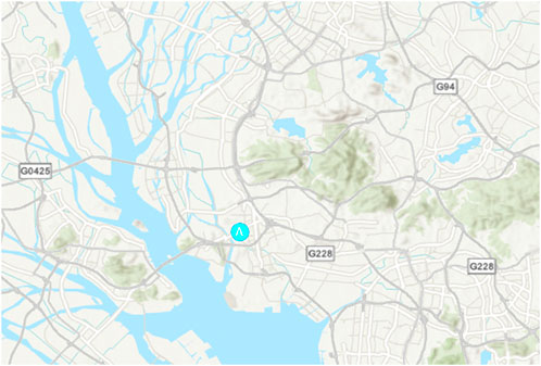
Figure 4. Geographical location of Chang’an town in dongguan city.

The dataset spans from 2015 to 2024 and includes 3,647 daily records of major air pollutants: PM_2.5, PM₁₀, NO₂, SO₂, CO, and O₃, alongside the AQI. PM_2.5, PM₁₀, NO₂, SO₂, CO, and O₃ are used as predictor variables, while AQI serves as the target variable. The data are sourced from official environmental monitoring platforms with high reliability and accuracy, ensuring the robustness of subsequent modeling tasks.

Situated in the core of the Greater Bay Area, Chang’an is surrounded by several industrial cities, and its air quality is influenced by both local emissions and regional pollutant transport, making it highly representative for studying industrial pollution dynamics. The results obtained here are expected to be generalizable to similar urban-industrial zones.

4.2 Descriptive statistics and feature analysis

4.2.1 Summary statistics

Descriptive statistics of AQI and major pollutant concentrations are presented in Table 1. The data show significant variability, especially in PM_2.5, PM₁₀, and O₃. The mean AQI is 66, indicating a moderate air quality level. However, its maximum value reaches 207, suggesting occasional severe pollution events. PM_2.5 and PM₁₀ exhibit high standard deviations, reflecting strong fluctuations in particulate matter concentrations. Although SO₂ and CO concentrations are generally low, CO values are relatively high during certain periods. NO₂ and O₃ also show considerable variability, revealing the complexity of air pollution in the region.

Table 1

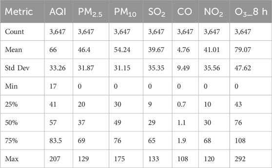
Table 1. Descriptive statistics of AQI and major pollutants (2015–2024).

Figure 5 illustrates the temporal evolution of AQI and pollutants. Several pollutants, especially SO₂, show noticeable fluctuations across years, providing a basis for understanding the temporal dynamics and episodic pollution patterns in Chang’an.

Figure 5

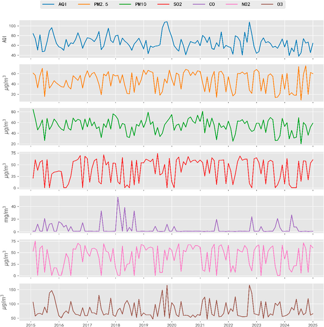
Figure 5. Time series trends of AQI and major pollutants (2015–2024).

4.2.2 Seasonal variation analysis

To capture seasonal patterns, Figure 6 presents the variations of AQI and pollutants across the four seasons: spring, summer, autumn, and winter. The red, blue, and purple curves represent the mean, maximum, and minimum values, respectively.

Figure 6

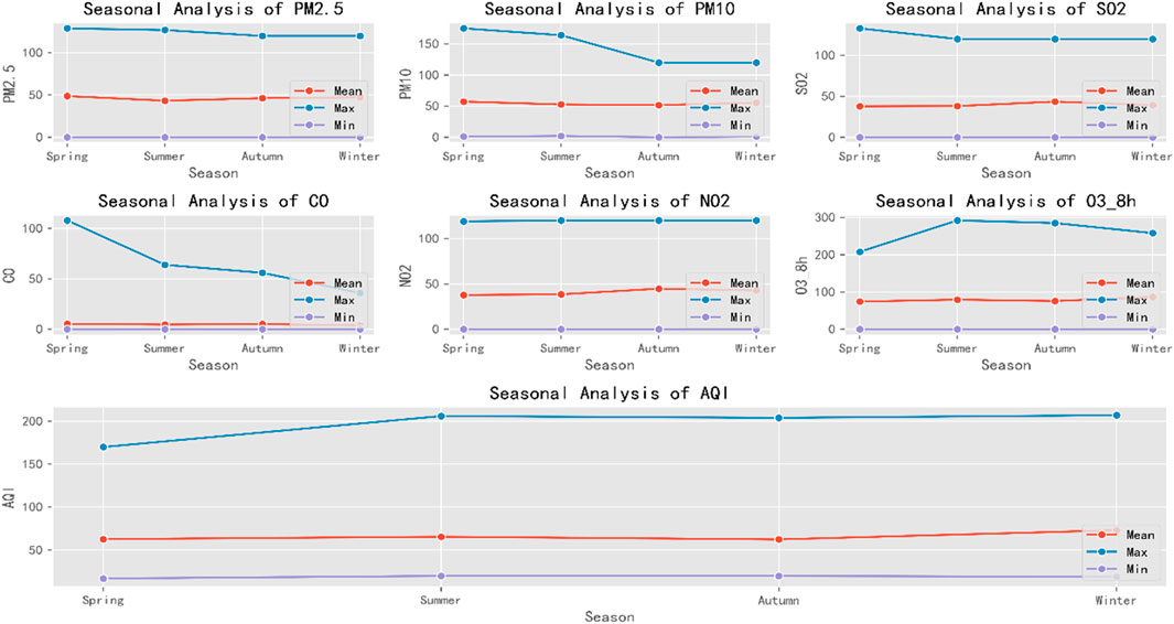
Figure 6. Seasonal patterns of AQI and major pollutants.

Overall, pollutants demonstrate distinct seasonal behaviors. PM₁₀ and O₃_8 h concentrations peak during summer, possibly due to intense solar radiation enhancing photochemical reactions. In contrast, CO levels rise sharply in winter, likely due to increased emissions from heating and poor atmospheric dispersion. AQI values also tend to be highest in winter, suggesting worse air quality conditions during this season. These patterns highlight the coupled influence of meteorological conditions on pollutant concentrations.

Table 2 shows the AQI classification used in China, as officially published by the Ministry of Ecology and Environment. This provides a regulatory context for interpreting the predicted AQI values. This classification serves as a basis for regulatory action and public health advisories, and also provides a meaningful benchmark for evaluating the performance of air quality forecasting models.

Table 2

Table 2. National AQI classification standard (China).

4.2.3 Data distribution

The histograms in Figure 7 show that AQI, PM_2.5, and PM₁₀ are right-skewed, with a significant peak at low values and a gradual decline afterward, indicating data concentration at the lower end. CO presents a sharp and narrow distribution, reflecting a highly consistent dataset. SO₂, NO₂ and O₃ exhibit more balanced or slightly left-skewed distributions, implying differences in their formation mechanisms.

Figure 7

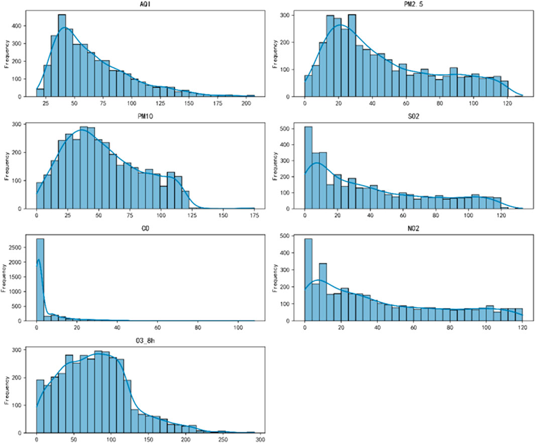
Figure 7. Frequency histograms of AQI and major pollutants.

4.2.4 Correlation analysis

Figure 8 illustrates the linear relationships among variables, quantified by Pearson correlation coefficients ranging from −1 (strong negative correlation) to +1 (strong positive correlation). The color gradient (red for positive, blue for negative) visually emphasizes the strength of each correlation. Notably, PM_2.5 and PM₁₀ demonstrate a moderately strong positive correlation (approximately 0.30), aligning with expectations for pollutants with shared emission sources and atmospheric dynamics. In contrast, O₃ shows weaker or even negative correlations with other pollutants, indicating a distinct generation mechanism and behavior. Most variable pairs exhibit low or negligible correlations, suggesting that their dynamics are influenced by different factors. These results can guide feature selection and variable engineering in subsequent regression and machine learning analyses.

Figure 8

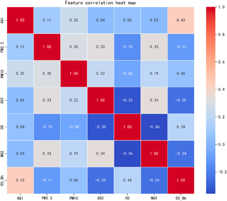
Figure 8. Pearson correlation coefficient heatmap.

Table 3 summarizes the statistical characteristics and normality test results for the AQI data. The AQI ranges from 17 to 207, with a mean of 66.01 and a standard deviation of 33.26, indicating substantial variability. The skewness value of 1.22 suggests a right-skewed distribution, while the kurtosis of 1.40, lower than the theoretical normal value of 3, indicates relatively light tail behavior. The Jarque–Bera test yields a statistic of 1,204.26 (p-value = 0.00), allowing for the rejection of the normality assumption at a significance level of 0.05. These results confirm that the AQI data deviates significantly from a normal distribution.

Table 3

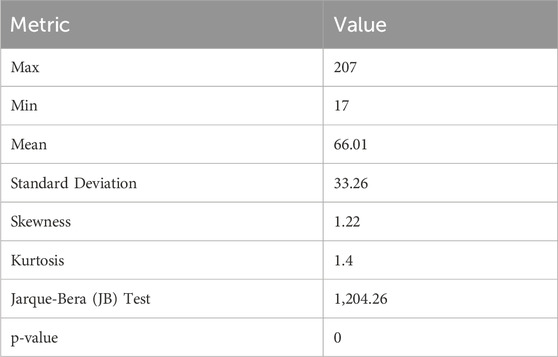
Table 3. Statistical characteristics of AQI and jarque–bera (JB) test results.

4.2.5 Stationarity testing

An Augmented Dickey–Fuller (ADF) test was conducted to assess the stationarity of the AQI time series. As shown in Figure 9, the ADF statistic is −8.9342, yielding a p-value of 0.0000, well below the significance threshold of 0.05. Thus, the null hypothesis of a unit root (non-stationarity) is rejected, confirming that the AQI series is stationary. This result supports the use of ARIMA models in subsequent baseline forecasting since they require stationary data.

Figure 9

Figure 9. Adf stationarity test results for the AQI time serie.

4.3 CEEMDAN decomposition of the AQI time series

Figure 10 presents the CEEMDAN decomposition results for the AQI series. CEEMDAN is an improved version of the EMD method. By introducing adaptive noise and performing ensemble averaging, CEEMDAN enhances the stability of the decomposition and improves the separation of modes. The first row (red) shows the original signal, which contains multiscale information, including high-frequency noise and low-frequency trends. The middle green subplots represent different IMFs, arranged from high to low frequencies. The higher-order IMFs capture high-frequency noise and fast oscillations, while the lower-order IMFs gradually reveal low-frequency trends. The final row represents the residual trend component, reflecting the long-term variations of the signal. CEEMDAN provides better decomposition performance than traditional EMD and EEMD (Ensemble Empirical Mode Decomposition), effectively suppressing mode mixing and yielding IMFs with clearer physical significance, making it possible to decompose the target prediction data into interpretable features. With feature engineering completed, the next step involves building the forecasting model and conducting experimental analysis.

Figure 10

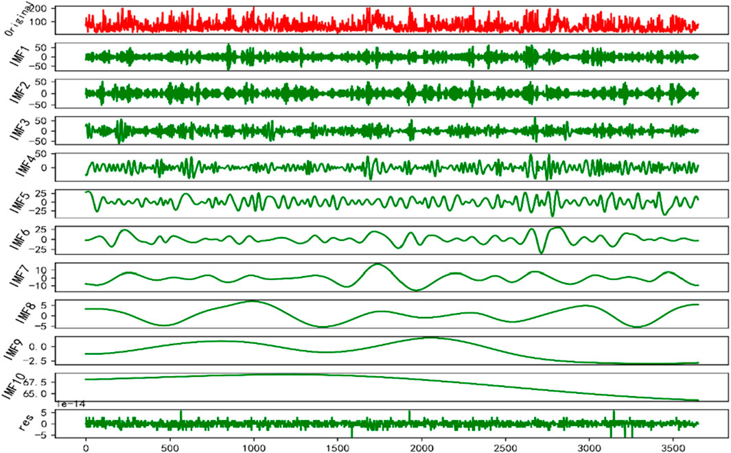
Figure 10. CEEMDAN decomposition of the AQI time series.

5 Results and discussion

5.1 Experimental environment and data processing

This study implemented the proposed CEEMDAN-GNN-Transformer and baseline models within a Python environment using the PyTorch deep learning framework. All experiments were conducted on a workstation configured with an NVIDIA GeForce RTX 3060 GPU, ensuring consistent training efficiency and reproducibility across experiments. Unless stated otherwise, all experiments were conducted under the same hardware and software conditions.

During the data preprocessing phase, the dataset was divided into training (80%) and test (20%) sets. The feature variables and prediction target were standardized using the StandardScaler method, yielding a mean of 0 and a standard deviation of 1 across both sets. This normalization mitigates the effects of differing variable scales, improves model training efficiency, and promotes stable convergence. The standardized data were then transformed into PyTorch tensors to enable high-performance batch processing within the deep learning pipelines.

5.2 Model evaluation metrics

To comprehensively assess the performance of the proposed model, this study adopts four widely used regression evaluation metrics: Mean Absolute Error (MAE), Mean Squared Error (MSE), Coefficient of Determination (R²), and Explained Variance Score (EVS). These metrics assess model performance from multiple perspectives, including error size, model fit, and the extent of data variance explanation (Chai and Draxler, 2014; Chicco et al., 2021).

MAE is the average of the absolute differences between actual observations and predicted values.

MSE is the mean of the squared differences between actual and predicted values.

R² quantifies the model’s ability to explain variance in the data, with values closer to 1 indicating better explanatory power.

EVS is similar to R² but focuses more on the model’s ability to explain data variability, with higher EVS values indicating better fit.

To comprehensively assess the performance of the models in air quality forecasting, four common regression metrics were selected: Mean Absolute Error (MAE), Mean Squared Error (MSE), Coefficient of Determination (R²), and Explained Variance Score (EVS). These metrics evaluate the model’s prediction performance from multiple dimensions, including error magnitude, goodness of fit, and its ability to capture the data’s variability. MAE measures the average absolute difference between the actual observations and the model’s predictions, while MSE captures the average squared error between actual and predicted values. The R² coefficient quantifies the proportion of data variance explained by the model, ranging from 0 to 1, with values closer to 1 indicating stronger explanatory capacity. EVS operates similarly to R² but focuses more explicitly on the proportion of data variance explained by the prediction, making it especially valuable for assessing the model’s ability to capture variability across the dataset.

5.3 Baseline models

To validate the effectiveness of the proposed CEEMDAN-GNN-Transformer model, this study selects nine representative predictive models for comparison. These models include deep learning approaches (e.g., CNN-Transformer), ensemble learning methods (e.g., XGBoost, GBDT, Random Forest), traditional machine learning methods (e.g., KNN, SVM), and classical time series models (e.g., ARIMA). These models exhibit significant differences in terms of time pattern modeling ability, variable relationship modeling strength, IMF component utilization, implementation complexity, and computational resource requirements, as summarized in Table 4 (Cui et al., 2023; Ye et al., 2025; Lei et al., 2023).

Table 4

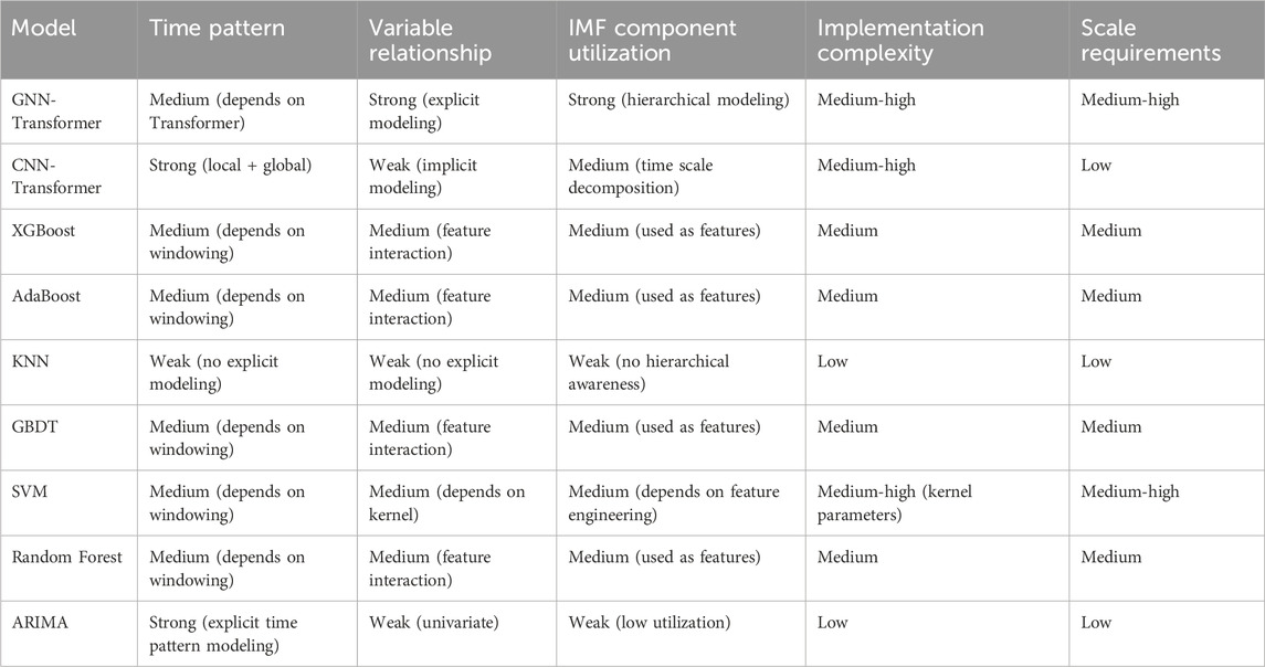
Table 4. GNN-transformer and baseline model feature comparison.

Through comparative analysis, it is evident that CNN-Transformer combines CNN’s local feature extraction ability and Transformer’s global dependency modeling capability, making it highly suitable for time series modeling. Compared to traditional time series models, CNN-Transformer efficiently extracts short-term patterns while modeling long-range dependencies, with relatively low computational complexity. By comparing it with GNN-Transformer, this study highlights the necessity of the GNN structure for temporal tasks and examines whether it enhances the Transformer’s performance in complex time series modeling. The comparison validates the advantage and applicability of GNN-Transformer in handling complex time series data and relational modeling tasks.

5.4 Ablation study

To explore the contribution of each key module in the proposed model and verify the combination effect, this study designs a systematic ablation experiment. Keeping hyperparameters consistent, the experiment sequentially removes or combines the signal decomposition module (CEEMDAN), the GNN, and the Transformer module, with a Multi-Layer Perceptron (MLP) used as the baseline model for comparison. Each experiment is repeated 20 times, with the average result taken to ensure robust and fair evaluation. The results are shown in Table 5.

Table 5

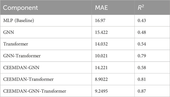
Table 5. Ablation experiment results comparison.

The experimental results indicate that both GNN and Transformer significantly improve the model’s performance. Transformer, in particular, demonstrates a more substantial effect (MAE reduced from 16.97 to 14.032, R² improved to 0.54). The combination of GNN and Transformer further enhances prediction capability (MAE reduced to 10.021, R² improved to 0.79), indicating a synergistic effect. Moreover, the introduction of CEEMDAN signal decomposition significantly optimizes the Transformer’s prediction performance (MAE reduced to 8.9022, R² improved to 0.81). When CEEMDAN is added on top of the GNN-Transformer combination, the performance improvement is limited (MAE decreases from 10.021 to 9.2495, R² improves to 0.87). In summary, the CEEMDAN-GNN-Transformer architecture demonstrates superior modeling capability in time series prediction tasks, with the complementary strengths of the three components achieving the best performance in complex temporal modeling tasks.

5.5 Hyperparameter optimization and model training

This study employs the Optuna framework for hyperparameter optimization, aiming to minimize the MSE of the GNN and Transformer models on the validation set. Optuna is a Bayesian optimization-based automated hyperparameter search tool that intelligently explores the search space to find the optimal combination of hyperparameters with the fewest trials. It supports various machine learning and deep learning frameworks, including Scikit-learn, PyTorch, and TensorFlow. By defining the search space, the optimizer selects appropriate hyperparameters such as the number of attention heads, hidden layer dimensions, model depth, learning rate, dropout rate, and number of neighbors. Through 50 trials, Optuna automatically tunes the hyperparameters to find the best combination, improving model prediction accuracy, reducing computational cost, and enhancing generalization ability.

Table 6 lists various hyperparameters affecting model performance, along with their respective search ranges. These include structural parameters (scaling factor for hidden layers, attention heads, and encoder layers), graph structure parameters (number of neighboring nodes in the graph), regularization parameters (dropout rate), and optimizer parameters (learning rate). The tuning of these hyperparameters directly impacts model training performance and generalization ability. After 20 iterations, the optimal combination of hyperparameters was obtained. A partial example of the optimization results is shown in Table 7.

Table 6

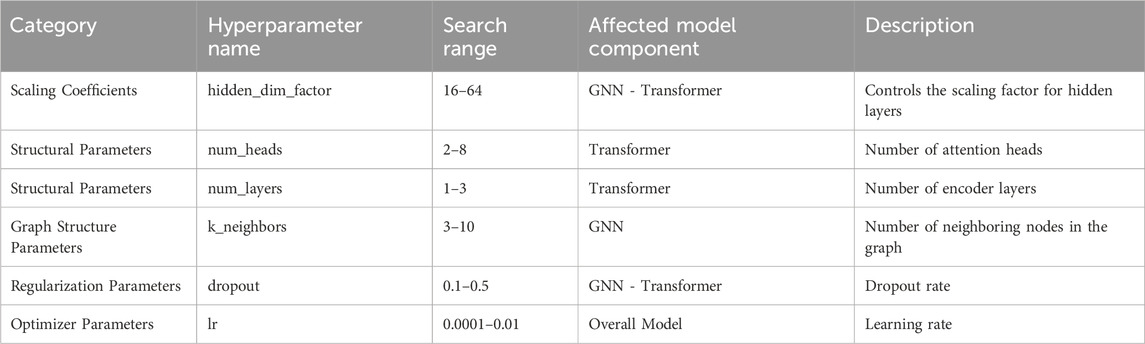
Table 6. Hyperparameter search space.

Table 7

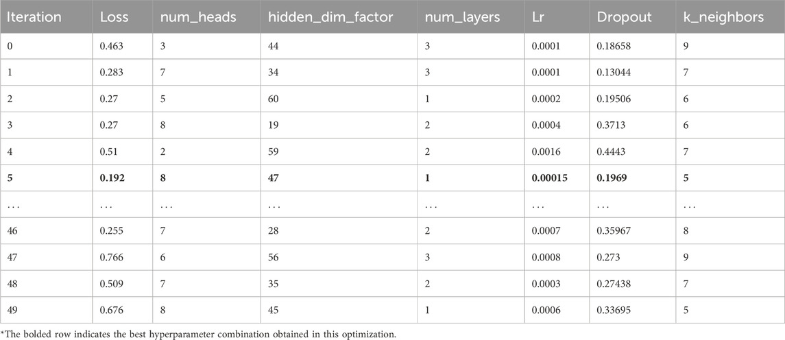
Table 7. Hyperparameter optimization results.

As shown in Table 7, the optimal hyperparameter combination found through the optimization process includes 8 attention heads, a hidden dimension scaling factor of 47, 1 attention layer, a learning rate of 0.000153, a dropout rate of 0.197, and 5 neighbors. This combination resulted in the best performance, with a loss of 0.1929, demonstrating the model’s best performance under these settings. The actual hidden layer dimension is calculated by multiplying the hidden_dim_factor by num_heads.

The final model was built using the best parameters obtained from Optuna’s optimization. The following steps were undertaken: the graph structure was constructed, with adjacency matrices calculated based on feature similarities for both the training and testing sets, where the k nearest neighbors were identified for each data point. The edge index for GNN computation was then built. The same k_neighbors value was used for both training and testing sets, but separate graph structures were created for each. The model was trained for 200 epochs. Each epoch included a forward pass through the GNN layers, Transformer layers, and a fully connected layer, followed by calculating the mean squared error loss between predicted and true values. Backpropagation was performed to compute gradients, and the Adam optimizer was used to update the model parameters.

From the training logs, as shown in Table 8, the loss decreases progressively over the training process, indicating that the model is converging and improving its prediction accuracy. The loss decreases rapidly during the initial stages (Epochs 20–40), from 0.3592 to 0.2892, reflecting the larger optimization steps in the early training phase. In subsequent stages, the loss stabilizes, indicating that the training process is becoming more stable. By Epoch 200, the loss converges to 0.1635. Overall, the decreasing trend in loss indicates the model’s effective training and suggests that it achieves an optimal performance level.

Table 8

Table 8. Model training loss progression.

Table 9 provides a summary of the final model’s parameter counts, highlighting its complexity and capacity.

Table 9

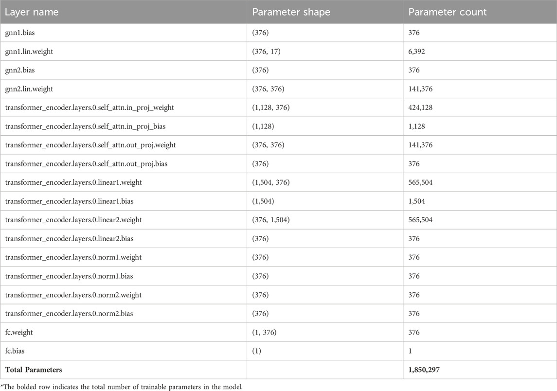
Table 9. Final model architecture and parameter counts.

The model developed in this study integrates a GNN and a Transformer architecture to process graph-structured data and capture global dependencies. The input feature dimension is 17, and after two layers of GNN processing, it is mapped to a 376-dimensional hidden representation. Subsequently, a single-layer Transformer encoder with 8 attention heads is used to further model global feature interactions. Finally, a fully connected layer maps the features to a 1-dimensional output for pollutant prediction. The total number of parameters is approximately 1.85 million, making it a relatively complex model for pollutant time series forecasting.

5.6 Forecasting results and comparative analysis

To comprehensively evaluate the forecasting performance of the proposed CEEMDAN–GNN–Transformer model for air quality prediction, a comparative analysis was conducted against a range of classical machine learning and deep learning approaches. All models were tested on the same dataset preprocessed via CEEMDAN signal decomposition, and their performance was assessed using four commonly used metrics: MAE, MSE, R², and EVS. The results are presented in Table 10.

Table 10

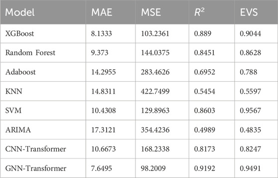
Table 10. Model performance comparison (based on CEEMDAN decomposition).

As shown in Table 10, the forecasting performances of the compared models vary significantly. The GNN–Transformer approach achieves the best results across all metrics, with the lowest MAE (7.6495) and MSE (98.2009), along with the highest R² (0.9192) and EVS (0.9491). This highlights its superior ability to capture complex temporal dynamics and to accurately explain the variance within the data. Meanwhile, XGBoost also delivers strong performance, yielding an R² of 0.8890 and an EVS of 0.9044, underscoring its effectiveness in capturing feature interactions and nonlinear relationships. In comparison, Random Forest, SVM, and CNN-Transformer perform slightly worse than XGBoost and GNN-Transformer in terms of MSE and MAE, while Adaboost and KNN show relatively weaker performance in all metrics. Notably, KNN has the highest MSE (422.7499) and the lowest R² (0.5454), which indicates its limitations in modeling complex dynamic relationships, especially in high-dimensional regression tasks. Overall, the GNN-Transformer and XGBoost models demonstrate superior prediction performance in this study, while traditional machine learning methods (e.g., KNN, Adaboost) show certain limitations in modeling complex dynamic changes.

Figure 11 illustrates the forecasting results of the GNN-Transformer model compared with observed AQI values. The predicted time series closely tracks the actual observations, demonstrating the model’s strong temporal modeling capability and its ability to capture long-term trends in air quality fluctuations. However, slight discrepancies are observed during certain extreme events, such as pollution peaks or sharp declines, where the predicted values tend to be smoother than the actual data. This limitation may arise from the signal decomposition and denoising process of CEEMDAN, which can attenuate high-frequency variations. Despite this, the proposed GNN-Transformer approach shows considerable promise in capturing the overall dynamics of air quality. In future work, incorporating meteorological covariates or further refining the model architecture could help better capture these abrupt variations and further improve prediction precision.

Figure 11

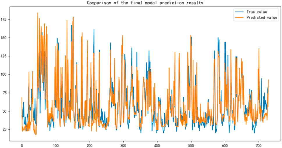
Figure 11. GNN-transformer model prediction fitting.

Although CEEMDAN is effective in reducing noise and extracting multi-scale features, its decomposition inherently introduces a smoothing bias, diminishing the retention of high-frequency signals. In this study, extreme pollution episodes (such as sharp AQI surges or declines) appear attenuated in the fitted curve. While beneficial for overall stability and trend extraction, this effect may be suboptimal for real-time air quality management, where timely detection of extreme events is critical for public health and emergency response. Future work could consider augmenting CEEMDAN with high-frequency component weighting or integrating auxiliary submodels optimized for peak detection to enhance responsiveness to short-term pollution shocks.

5.7 Model uncertainty quantification and prediction interval evaluation

In environmental air quality forecasting, beyond accuracy, it is equally important to quantify the uncertainty of predictions, as this information supports scientific decision-making and risk management. To this end, the Monte Carlo (MC) Dropout method—a Bayesian approximation technique—was applied to the CEEMDAN–GNN–Transformer model for uncertainty analysis.

Originally proposed by Gal and Ghahramani. (2016), MC Dropout involves keeping the dropout mechanism active during inference, performing multiple stochastic forward passes to simulate sampling from the posterior weight distribution. This enables approximate estimation of the predictive distribution. For each of T stochastic passes, predictions $\widehat{{\mathrm{y}}_{\mathrm{t}}}$ are collected, from which the predictive mean and variance are computed, as shown in Equations 15, 16:

$\mathrm{E}\left[\widehat{{\mathrm{y}}^{*}}\right]\approx \frac{1}{\mathrm{T}}{\displaystyle \sum _{\mathrm{t}=1}^{\mathrm{T}}}\widehat{{\mathrm{y}}_{\mathrm{t}}}(15)$

$\text{Var}\left[\widehat{{\mathrm{y}}^{*}}\right]\approx \frac{1}{\mathrm{T}}{\displaystyle \sum _{\mathrm{t}=1}^{\mathrm{T}}}{\left(\widehat{{\mathrm{y}}_{\mathrm{t}}}-\mathrm{E}\left[\widehat{{\mathrm{y}}^{*}}\right]\right)}^2(16)$

Using these results, two uncertainty evaluation metrics were calculated: Prediction Interval Coverage Probability (PICP) and Mean Prediction Interval Width (MPIW). The results are shown in Table 11.

Table 11

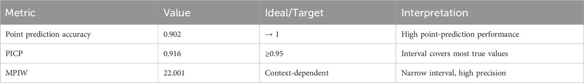
Table 11. Bayesian approximation–based uncertainty evaluation.

The results show that the PICP (0.916) is close to the ideal 95% coverage, indicating that the prediction intervals successfully cover the majority of observed values. The MPIW (22.001) is substantially narrower than the typical AQI category width (≈50 for mild pollution), implying high-precision prediction intervals.

6 Conclusion

This study addresses the forecasting of the AQI in Changan Town, Dongguan, and proposes an improved CEEMDAN–GNN–Transformer framework aimed at enhancing both prediction accuracy and stability. First, the AQI time series is decomposed using the CEEMDAN method, extracting multi-scale features and mitigating the effects of non-stationarity in the original data. Second, a GNN is introduced to capture spatial dependencies, effectively uncovering latent spatial relationships among various pollutants and environmental factors, thereby enhancing the model’s ability to perceive the evolution patterns of AQI. Finally, a Transformer module is employed to model long-term temporal dependencies, capturing the temporal dynamics and trend characteristics of AQI variations.

Through ablation experiments and hyperparameter optimization, this study validated the contribution of each submodule to the overall model performance and compared it with several mainstream baseline models. The experimental results show that the proposed CEEMDAN-GNN-Transformer model outperforms all other models across all evaluation metrics (MAE, MSE, R², EVS), with particularly significant advantages in prediction accuracy and fitting ability. Specifically, the model achieved the lowest MAE (7.6495) and MSE (98.2009), an R² of 0.9192, and an EVS of 0.9491, demonstrating that this approach can accurately capture the long-term evolution characteristics of AQI and improve the reliability and stability of the prediction results.

From a deployment perspective, the CEEMDAN–GNN–Transformer model demonstrates manageable hardware requirements. Experiments indicate that training and inference can be completed within a reasonable time frame on a mid-range GPU (NVIDIA RTX 3060), making it viable for implementation in local environmental monitoring centers or regional environmental agencies. However, several limitations remain: (1) current inputs are limited to pollutant concentration data, without incorporating meteorological conditions or emission source activity, which may reduce accuracy during extreme pollution events; (2) the smoothing effect of CEEMDAN, while improving stability, may weaken sensitivity to short-term abrupt changes; and (3) cross-regional generalization has yet to be validated with multi-city, multi-station datasets.

Future work will focus on integrating multi-source data (e.g., meteorological variables, traffic flow) and introducing weighted enhancement strategies for high-frequency components to balance long-term trend forecasting with short-term anomaly detection. Furthermore, interpretability methods will be incorporated—leveraging attention weight distributions and feature attribution rankings—to systematically analyze the relative contributions of pollutants and environmental factors, thereby improving transparency and application value. Finally, the model will be tested across diverse regional settings to promote its practical adoption in real-time AQI early warning and long-term trend prediction.

Data availability statement

The original contributions presented in the study are included in the article/Supplementary Material, further inquiries can be directed to the corresponding authors.

Author contributions

SH: Conceptualization, Methodology, Writing – original draft, Writing – review and editing, Funding acquisition. YL: Investigation, Data curation, Writing – review and editing. JP: Formal analysis, Data curation, Writing – review and editing. DX: Supervision, Resources, Writing – review and editing. YW: Methodology, Data curation, Writing – review and editing.

Funding

The author(s) declare that financial support was received for the research and/or publication of this article. This research was supported by the following projects: the Doctoral Research Start-up Fund Project of Guangdong University of Science and Technology (Grant No. GKY-2024BSQDW-6), the Project of China Business Statistics Society (Grant No. 2024STY118), the Guangdong Social Science Fund Special Project “Mechanism of Original Innovation in Emerging Leading Industries in the Guangdong-Hong Kong-Macao Greater Bay Area” (Grant No. GD24DWQGL01), the Guangdong Basic and Applied Basic Research Joint Fund Project “The Role of the Guangdong-Dongguan Joint Fund in Promoting Regional Original Innovation” (Grant No. 2023A1515140047), the Guangdong Philosophy and Social Science Planning Co-construction Project “Policy Perception and Simulation of the Digital Transformation of Manufacturing in Guangdong Province” (Grant No. GD23XGL052), and the Dongguan Philosophy and Social Science Planning General Project “Development Path and Practical Strategies of Manufacturing Aesthetics in Dongguan from the Perspective of the Digital Economy Empowerment” (Grant No. 2025CG105).

Conflict of interest

The authors declare that the research was conducted in the absence of any commercial or financial relationships that could be construed as a potential conflict of interest.

Generative AI statement

The author(s) declare that no Generative AI was used in the creation of this manuscript.

Any alternative text (alt text) provided alongside figures in this article has been generated by Frontiers with the support of artificial intelligence and reasonable efforts have been made to ensure accuracy, including review by the authors wherever possible. If you identify any issues, please contact us.

Publisher’s note

All claims expressed in this article are solely those of the authors and do not necessarily represent those of their affiliated organizations, or those of the publisher, the editors and the reviewers. Any product that may be evaluated in this article, or claim that may be made by its manufacturer, is not guaranteed or endorsed by the publisher.

Supplementary material

The Supplementary Material for this article can be found online at: https://www.frontiersin.org/articles/10.3389/fenvs.2025.1653446/full#supplementary-material

References

Abirami, S., and Chitra, P. (2021). Regional air quality forecasting using spatiotemporal deep learning. J. Clean. Prod. 283, 125341. doi:10.1016/j.jclepro.2020.125341

CrossRef Full Text | Google Scholar

Agbehadji, I. E., and Obagbuwa, I. C. (2024). Systematic review of machine learning and deep learning techniques for spatiotemporal air quality prediction. Atmosphere 15 (11), 1352. doi:10.3390/atmos15111352

CrossRef Full Text | Google Scholar

Ameri, R., Hsu, C. C., Band, S. S., Zamani, M., Shu, C. M., and Khorsandroo, S. (2023). Forecasting PM 2.5 concentration based on integrating of CEEMDAN decomposition method with SVM and LSTM. Ecotoxicol. Environ. Saf. 266, 115572. doi:10.1016/j.ecoenv.2023.115572

PubMed Abstract | CrossRef Full Text | Google Scholar

Ban, W., and Shen, L. (2022). PM2. 5 prediction based on the CEEMDAN algorithm and a machine learning hybrid model. Sustainability 14 (23), 16128. doi:10.3390/su142316128

CrossRef Full Text | Google Scholar

Chai, T., and Draxler, R. R. (2014). Root mean square error (RMSE) or mean absolute error (MAE)? Arguments against avoiding RMSE in the literature. Geosci. Model Dev. 7 (3), 1247–1250. doi:10.5194/gmd-7-1247-2014

CrossRef Full Text | Google Scholar

Chen, Y., Chen, X., Xu, A., Sun, Q., and Peng, X. (2022). A hybrid CNN-Transformer model for ozone concentration prediction. Air Qual. Atmos. and Health 15 (9), 1533–1546. doi:10.1007/s11869-022-01197-w

CrossRef Full Text | Google Scholar

Chen, L., Xu, J., Wu, B., and Huang, J. (2023). Group-aware graph neural network for nationwide city air quality forecasting. ACM Trans. Knowl. Discov. Data 18 (3), 1–20. doi:10.1145/3631713

PubMed Abstract | CrossRef Full Text | Google Scholar

Chicco, D., Warrens, M. J., and Jurman, G. (2021). The coefficient of determination R-squared is more informative than SMAPE, MAE, MAPE, MSE and RMSE in regression analysis evaluation. Peerj Comput. Sci. 7, e623. doi:10.7717/peerj-cs.623

PubMed Abstract | CrossRef Full Text | Google Scholar

Cui, B., Liu, M., Li, S., Jin, Z., Zeng, Y., and Lin, X. (2023). Deep learning methods for atmospheric PM2. 5 prediction: a comparative study of transformer and CNN-LSTM-attention. Atmos. Pollut. Res. 14 (9), 101833. doi:10.1016/j.apr.2023.101833

CrossRef Full Text | Google Scholar

Gal, Y., and Ghahramani, Z. (2016). Dropout as a bayesian approximation: representing model uncertainty in deep learning. In: International conference on machine learning. Dongguan, China: University of Science and Technology. p. 1050–1059.

Google Scholar

Ge, L., Wu, K., Zeng, Y., Chang, F., Wang, Y., and Li, S. (2021). Multi-scale spatiotemporal graph convolution network for air quality prediction. Appl. Intell. 51, 3491–3505. doi:10.1007/s10489-020-02054-y

CrossRef Full Text | Google Scholar

Guangdong Provincial Department of Ecology and Environment (2023). Guangdong ecological and environmental bulletin 2022 [in Chinese]. Guangzhou: Guangdong Provincial Department of Ecology and Environment.

Google Scholar

Guo, C., Kang, X., Xiong, J., and Wu, J. (2023). A new time series forecasting model based on complete ensemble empirical mode decomposition with adaptive noise and temporal convolutional network. Neural Process. Lett. 55 (4), 4397–4417. doi:10.1007/s11063-022-11046-7

PubMed Abstract | CrossRef Full Text | Google Scholar

He, S., Jang, G., and Liu, Y. (2025). Hybrid transformer-TimesNet model for accurate prediction of industrial air pollutants: a case study of the xinyang industrial zone, China. Pol. J. Environ. Stud. 152, 203348. doi:10.15244/pjoes/203348

CrossRef Full Text | Google Scholar

Horn, S. A., and Dasgupta, P. K. (2024). The Air Quality Index (AQI) in historical and analytical perspective a tutorial review. Talanta 267, 125260. doi:10.1016/j.talanta.2023.125260

PubMed Abstract | CrossRef Full Text | Google Scholar

Hu, M., Zhang, S., Dong, W., Xu, F., and Liu, H. (2021). Adaptive denoising algorithm using peak statistics-based thresholding and novel adaptive complementary ensemble empirical mode decomposition. Inf. Sci. 563, 269–289. doi:10.1016/j.ins.2021.02.040

CrossRef Full Text | Google Scholar

Kumbalaparambi, T. S., Menon, R., Radhakrishnan, V. P., and Nair, V. P. (2023). Assessment of urban air quality from Twitter communication using self-attention network and a multilayer classification model. Environ. Sci. Pollut. Res. 30 (4), 10414–10425. doi:10.1007/s11356-022-22836-w

PubMed Abstract | CrossRef Full Text | Google Scholar

Lei, T. M., Ng, S. C., and Siu, S. W. (2023). Application of ANN, XGBoost, and other ml methods to forecast air quality in Macau. Sustainability 15 (6), 5341. doi:10.3390/su15065341

CrossRef Full Text | Google Scholar

Li, Y., Guo, J. E., Sun, S., Li, J., Wang, S., and Zhang, C. (2022). Air quality forecasting with artificial intelligence techniques: a scientometric and content analysis. Environ. Model. and Softw. 149, 105329. doi:10.1016/j.envsoft.2022.105329

CrossRef Full Text | Google Scholar

Liang, Y., Xia, Y., Ke, S., Wang, Y., Wen, Q., Zhang, J., et al. (2023). Airformer: predicting nationwide air quality in China with transformers. Proc. AAAI Conf. Artif. Intell. 37 (12), 14329–14337. doi:10.1609/aaai.v37i12.26676

CrossRef Full Text | Google Scholar

Liu, H., Yan, G., Duan, Z., and Chen, C. (2021). Intelligent modeling strategies for forecasting air quality time series: a review. Appl. Soft Comput. 102, 106957. doi:10.1016/j.asoc.2020.106957

CrossRef Full Text | Google Scholar

Mishra, A., and Gupta, Y. (2024). Comparative analysis of Air Quality Index prediction using deep learning algorithms. Spatial Inf. Res. 32 (1), 63–72. doi:10.1007/s41324-023-00541-1

CrossRef Full Text | Google Scholar

Sharma, V., Ghosh, S., Mishra, V. N., and Kumar, P. (2025). Spatio-temporal Variations and Forecast of PM2. 5 concentration around selected Satellite Cities of Delhi, India using ARIMA model. Phys. Chem. Earth, Parts A/B/C 138, 103849. doi:10.1016/j.pce.2024.103849

CrossRef Full Text | Google Scholar

Tang, C., Wang, Z., Wei, Y., Zhao, Z., and Li, W. (2024). A novel hybrid prediction model of air quality index based on variational modal decomposition and CEEMDAN-SE-GRU. Process Saf. Environ. Prot. 191, 2572–2588. doi:10.1016/j.psep.2024.10.018

CrossRef Full Text | Google Scholar

Vaswani, A., Shazeer, N., Parmar, N., Uszkoreit, J., Jones, L., Gomez, A. N., et al. (2017). Attention is all you need. Adv. Neural Inf. Process. Syst. 30.

Google Scholar

Wang, Z., Wu, X., and Wu, Y. (2023). A spatiotemporal XGBoost model for PM2. 5 concentration prediction and its application in Shanghai. Heliyon 9 (12), e22569. doi:10.1016/j.heliyon.2023.e22569

PubMed Abstract | CrossRef Full Text | Google Scholar

Wu, Z., Zhao, W., and Lv, Y. (2022). An ensemble LSTM-based AQI forecasting model with decomposition-reconstruction technique via CEEMDAN and fuzzy entropy. Air Qual. Atmos. and Health 15 (12), 2299–2311. doi:10.1007/s11869-022-01252-6

PubMed Abstract | CrossRef Full Text | Google Scholar

Wu, X., Zhu, J., and Wen, Q. (2024). Short-term prediction of PM2. 5 concentration by hybrid neural network based on sequence decomposition. Plos one 19 (5), e0299603. doi:10.1371/journal.pone.0299603

PubMed Abstract | CrossRef Full Text | Google Scholar

Ye, Y., Cao, Y., Dong, Y., and Yan, H. (2025). A Graph Neural Network and Transformer-based model for PM2. 5 prediction through spatiotemporal correlation. Environ. Model. and Softw. 191, 106501. doi:10.1016/j.envsoft.2025.106501

CrossRef Full Text | Google Scholar

Zaini, N. A., Ean, L. W., Ahmed, A. N., and Malek, M. A. (2022). A systematic literature review of deep learning neural network for time series air quality forecasting. Environ. Sci. Pollut. Res. 29, 4958–4990. doi:10.1007/s11356-021-17442-1

PubMed Abstract | CrossRef Full Text | Google Scholar

Zhang, Z., and Zhang, S. (2023). Modeling air quality PM2. 5 forecasting using deep sparse attention-based transformer networks. Int. J. Environ. Sci. Technol. 20 (12), 13535–13550. doi:10.1007/s13762-023-04900-1

CrossRef Full Text | Google Scholar

Zhang, L., Liu, J., Feng, Y., Wu, P., and He, P. (2023). PM2. 5 concentration prediction using weighted CEEMDAN and improved LSTM neural network. Environ. Sci. Pollut. Res. 30 (30), 75104–75115. doi:10.1007/s11356-023-27630-w

PubMed Abstract | CrossRef Full Text | Google Scholar

Zhou, J., Cui, G., Hu, S., Zhang, Z., Yang, C., Liu, Z., et al. (2020). Graph neural networks: a review of methods and applications. AI open 1, 57–81. doi:10.1016/j.aiopen.2021.01.001

CrossRef Full Text | Google Scholar