Flood susceptibility mapping in El Niño Phenomenom integrating multitemporal radar analysis, GIS and machine learning techniques, Piura river basin, Peru

Floods represent the most frequent natural hazard, generating significant impacts on people as well as considerable economic and environmental losses worldwide. These events are particularly exacerbated by extreme climatic phenomena, such as the 2017 Coastal El Niño, the most intense in the past century, with the Piura region of Peru being the most affected. Flood susceptibility mapping (FSM) are essential for mitigating the negative impacts of floods through land-use planning, policy and plan formulation, and fostering community resilience for the sustainable occupation and use of floodplains. This study aimed to develop FSM in northern Peru, particularly in the Piura region, using a hybrid methodology integrating optical and radar remote sensing (RS), GIS, and machine learning (ML) techniques. Sentinel-1 data were used to map flood extent using the Normalized Difference Flood Index (NDFI), while flood susceptibility was modeled using ten topographic variables (derived from a DEM), the Normalized Difference Vegetation Index (NDVI), geology, and geomorphology; issues related to correlation and multicollinearity among topographic variables were addressed through Principal Component Analysis (PCA), selecting four principal components that explained 75.4% of the variance. Six FSMs were generated using Support Vector Machine (SVM) and Random Forest (RF), combined with different methods to estimate the quantitative relationship between variables and flood occurrence: Quantiles (q), Frequency Ratio (FR), and Weights of Evidence (WoE) (SVM-q, SVM-FR, SVM-WoE, RF-q, RF-FR, and RF-WoE). Model validation was performed using metrics such as the Area Under the ROC Curve (AUC), F1-score, and Accuracy, along with a cross-validation analysis. The results revealed that the RF ensemble model with WoE (RF-WoE) exhibited the best performance (AUC = 0.988 in training and >0.907 in validation), outperforming the SVM-based models; the SHAP analysis confirmed the significance of geology, geomorphology, and aspect in flood prediction. The resulting susceptibility maps identified the lower Piura River basin as the most vulnerable area, particularly during the 2017 Coastal El Niño event, due to morphological factors and inadequate land occupation. This study contributes to the field by demonstrating the effectiveness of a hybrid methodology that combines PCA, machine learning, and SHAP analysis, providing a more robust and interpretable approach to flood susceptibility mapping. Finally, the findings provide valuable inputs for local authorities, decision-makers, and organized communities to strengthen resilience, reduce vulnerability, and enhance preparedness against future floods, while also supporting the formulation of public policies and the integration of flood susceptibility into land-use planning for sustainable territorial management.

1 Introduction

In recent decades, the global climate has experienced a significant increase in temperatures, a phenomenon that has intensified extreme weather patterns, including prolonged droughts and intense precipitation events (Coumou and Rahmstorf, 2012; IPCC, 2021). This warming trend increases the specific humidity of the atmosphere, while relative humidity remains nearly constant, leading to a greater availability of atmospheric moisture (Koutsoyiannis, 2020). Consequently, this increase in the capacity of warm air to retain greater amounts of water vapor has exacerbated the frequency and intensity of floods, particularly in vulnerable regions (Benoudjit, 2020).

Floods are defined as hydrometeorological or ocean-origin events that inundate normally dry areas (Doswell, 2015; Rodriguez De La Cruz and Moreno Arqque, 2023), manifest in various forms, including pluvial, fluvial, and flash floods (Towfiqul Islam et al., 2021; Bentivoglio et al., 2022); these events represent the most frequent natural hazard worldwide, accounting for 43.4% of recorded disasters and affecting approximately two billion people, equivalent to 45% of the global population (Doswell, 2015; Benoudjit, 2020; Michaelides, 2021; Pradhan et al., 2023; EM-DAT, 2025). Additionally, floods rank third in terms of economic losses over the past 2 decades, surpassed only by storms and earthquakes (Pascaline and Rowena, 2018). Their impacts go beyond economic damage, affecting social, cultural, and ecological systems by destroying infrastructure, agricultural lands, and livelihoods (Tehrany et al., 2014a; Cian et al., 2018a; Ahmed et al., 2023); furthermore, floods can transport contaminants that degrade the quality of surface and groundwater, leading to negative consequences for human health and ecosystems (Khosravi et al., 2019; Benoudjit, 2020). Nevertheless, floodplains, characterized by their high fertility due to nutrient deposition and moisture retention, have historically played a crucial role in agricultural development (Doswell, 2015).

Historically, the Peruvian coast has been affected by episodes of the El Niño Phenomenon or the El Niño-Southern Oscillation (ENSO), which are natural ocean-atmosphere interaction events occurring in regions 3.4 and 1 + 2, the latter being associated with Coastal El Niño in the Equatorial Pacific Ocean (SENAMHI, 2014). In the last five centuries, at least 120 El Niño episodes have been recorded (Quinn et al., 1987; SENAMHI, 2014), three of which have been classified as extraordinarily intense and have occurred within the last 40 years, including the 2017 Coastal El Niño event (INDECI, 2017). ENSO events trigger an abrupt rise in sea surface temperature and torrential rainfall, causing daily river discharges to increase by up to 500% in the northwestern watershed. In northern Peru, these events periodically disrupt territorial development processes, disproportionately affecting impoverished populations due to the occurrence of landslides, debris flows, flash floods, storms, floods, pest outbreaks, and epidemics (Rodríguez-Morata et al., 2019; Molleda and Velásquez Serra, 2024). The economic losses from the last three ENSO events amounted to $3.283 billion in 1982/1983, $3.5 billion in 1997/1998 (SENAMHI, 2014), and $4.8 billion in 2017 (Gestión, 2018). The 2017 event is considered the third most intense El Niño event in Peru in at least the past 100 years (ENFEN, 2017), therefore, areas vulnerable to recurrent flooding due to ENSO events must be effectively managed to assess, prevent, and mitigate disaster risks.

The reliable determination of flood extent during extreme events such as ENSO, at the watershed scale, is a valuable tool for decision-making, enabling the reduction, management, and mitigation of flood-related losses (Towfiqul Islam et al., 2021; Pedzisai et al., 2023). Several studies have delineated flood extent using approaches such as field observations supported by geographic information systems (GIS) and RS (Cian et al., 2018b; Singh and Kansal, 2022). Over the past decades, the accessibility of free optical and radar imagery has significantly improved the accuracy of flood mapping. However, in the case of optical imagery, cloud cover poses a limitation during extreme flooding events, whereas radar imagery remains unaffected by meteorological conditions (Xue et al., 2022; Pedzisai et al., 2023). Therefore, to accurately map the historical extent of flooding during the 2017 Coastal ENSO event—a period characterized by persistent cloud cover—the Normalized Difference Flood Index (NDFI) was applied using radar imagery (Cian et al., 2018a); this method, commonly used to delineate open water and inundated vegetation in similar environments, provides a reliable dataset on flood dimensions. Another approach involves reconstructing flood extent through hydrodynamic modeling (Afshari et al., 2018; Zhang et al., 2022), which requires field data for model calibration and is computationally expensive (Teng et al., 2017; Kumar et al., 2023), making it challenging to implement in data-scarce regions like our study area. In recent years, there has been a surge in modeling flood extent and water levels using artificial intelligence (AI) and machine learning (ML) techniques, which include various classification and regression algorithms such as random forest (RF), Support Vector Machine (SVM), naive Bayes (NB), and gradient boosting (GB), multilayer perceptron (MLP), among others (Towfiqul Islam et al., 2021; Brill, 2022; Elkhrachy, 2022; Chen et al., 2023; Uzzal Mia et al., 2023). As highlighted by Rozos et al. (2022), the application of ML models in hydrology is well established, not only for direct flood mapping but also for assessing the performance of hydrological models, offering a computationally efficient and robust alternative to traditional evaluation methods. These approaches enable the objective handling of complex nonlinear problems while covering large study areas at a lower computational cost (Zhao et al., 2024).

On the other hand, flood susceptibility mapping have been significantly improved, ranging from qualitative methods such as the geomorphological approach (CORCUENCAS, 2014), to semi-quantitative approaches employing hierarchical analysis processes or multi-criteria analysis (Van Westen et al., 2003; Vilchez et al., 2013), and quantitative statistical models such as frequency ratio and weight of evidence methods (Rahmati et al., 2016; Natarajan et al., 2021). Additionally, machine learning-based flood susceptibility mapping (Al-Aizari et al., 2022; Elkhrachy, 2022), including hybrid approaches (Tehrany et al., 2014b; Shafizadeh-Moghadam et al., 2018; Towfiqul Islam et al., 2021), have demonstrated higher accuracy and lower bias (Singha et al., 2022) compared to traditional models. However, their widespread adoption by stakeholders has been limited due to their black-box nature (Pradhan et al., 2023). This issue is being addressed by quantifying the contribution of each variable to machine learning-based flood susceptibility mapping using the SHapely Additive exPlanations (SHAP) method proposed by Lundberg and Lee, (2017).

Although ML has been increasingly applied to FSM, many models still operate as black boxes, limiting their interpretability and practical application. Moreover, few studies have explored hybrid approaches in ENSO-affected regions, and even fewer have incorporated explainable AI techniques such as SHAP to enhance model transparency. This study addresses these gaps by integrating SAR-based flood mapping, hybrid machine learning approaches, and SHAP analysis, providing a comprehensive and interpretable methodology to support flood risk management. In this context, this research has two main objectives: first, to map the flooded areas during the 2017 Coastal ENSO event using the NDFI applied to radar imagery, following the approach proposed by Cian et al. (2018a); and second, to identify the areas most susceptible to flooding through the application of ML models, including Random Forest (RF) and Support Vector Machine (SVM), both in their simple forms (RF-q, SVM-q) and in hybrid approaches combined with Frequency Ratio (RF-FR and SVM-FR) and Weights of Evidence (RF-WoE and SVM-WoE). Additionally, the SHAP method was employed to quantify the contribution of each variable in the susceptibility models, providing greater transparency and robustness to the results. Ultimately, this study seeks to contribute to flood risk management in northern Peru by providing innovative, accurate, and interpretable tools to strengthen resilience, support land-use planning, and inform disaster risk reduction strategies.

2 Materials and methods

2.1 Study area

The department of Piura is located in the most northwestern region of Peru, between 4.089° and 6.372° south latitude and 81.328° and 79.210° west longitude. It covers an area of 35,837.6 km² and borders the department of Tumbes to the north, Ecuador and the department of Cajamarca to the east, the department of Lambayeque to the south, and the Pacific Ocean to the west (Figure 1). Elevations in Piura range from sea level to 3,881 m a.s.l., with two distinct altitudinal zones: a coastal plain in the western sector, below 400 m a.s.l., characterized by slopes of less than 5°, and an eastern foothill zone of the Andes Mountains (Vilchez et al., 2013), extending from 400 m a.s.l. to approximately 3,860 m a.s.l. More than 70% of the lithology in Piura consists primarily of loose to semi-consolidated soils, with a predominance of alluvial, fluvial, and aeolian deposits composed of sands and gravels. Additionally, to a lesser extent, the region contains volcanic-sedimentary rocks, intrusive rock outcrops, clastic or carbonate sedimentary rocks, and metamorphic formations (Vilchez et al., 2013; INGEMMET, 2023). From a geomorphological perspective, alluvial plains or floodplains are the predominant landforms, followed by geomorphological units of hills and low ridges, and finally mountain units. Although Piura is located near the equatorial line, which suggests a warm, humid climate with high precipitation, the Andes Mountains and the Humboldt and El Niño currents significantly modify the climatic conditions, creating a climate with distinct characteristics (Vilchez et al., 2013). According to the climate classification by Thornthwaite, the region of Piura exhibits eleven climate types. The most extensive is the arid type, which is characterized by moisture deficiency throughout the year. Precipitation in this zone ranges from 20 mm to 50 mm in the Sechura Desert and increases to values between 700 mm and 900 mm in the interior and highland areas of Piura. Additionally, the region includes a semiarid climate with annual precipitation between 200 mm and 500 mm, as well as a rainy climate in the highest elevations, where precipitation can reach up to 3000 mm per year (SENAMHI, 2020).

Figure 1

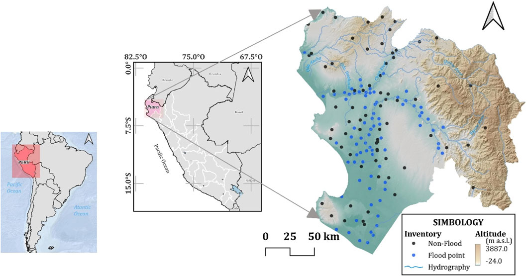
Figure 1. Map ubication of the study area.

In the region of Piura, ENSO, and Coastal ENSO occur periodically, altering meteorological conditions depending on their intensity and duration. During the extraordinary ENSO events of 1982/1983, 1997/1998, and 2016/2017, extreme precipitation was recorded, ranging from 1,000 mm per quarter to 3000 mm between September and May. The highest rainfall concentrations were observed in Piura, with precipitation anomalies exceeding 2000% (SENAMHI, 2014; INGEMMET, 2023), these anomalies triggered floods and mass movement processes, leading to significant socio-economic impacts, including loss of human lives, dehydration, hunger, disease outbreaks, and damage or destruction of housing, infrastructure, and livelihoods. The most affected sectors included agriculture, livestock, industry, mining, fishing, transportation, and electricity, among others. At the national level, economic losses in terms of Gross Domestic Product (GDP) were 7.0%, 4.5%, and 1.5% for the El Niño events of 1982/1983, 1997/1998, and 2016/2017, respectively (Galarza et al., 2012; COMEXPERÚ, 2024). In Piura and Tumbes, 85% of agriculture was irreparably lost, with estimated losses of 10 billion soles in crops such as banana, rice, and soy; additionally, Piura was the most affected region, with 28,560 damaged homes, the largest loss of crop hectares, and the greatest impact on infrastructure (Galarza et al., 2012). The 2017 event, classified as the most intense in the last 100 years, confirmed Piura as the most severely affected region (Scipión et al., 2018), therefore, it is crucial to map fluvial and pluvial floods at a regional scale in both urban and rural areas of Piura during extraordinary events. This mapping will enable risk assessment and the establishment of effective measures for disaster reduction, preparedness, response, rehabilitation, and reconstruction, thus mitigating catastrophic impacts on the population, livelihoods, and infrastructure.

2.2 Data

Table 1 presents the data used in this research. All variables were standardized to the same spatial resolution of 30 m per pixel, including geological and environmental variables, and the scale of the susceptibility mapping was 1:10,000. All input variables are shown in Figure A1.

Table 1

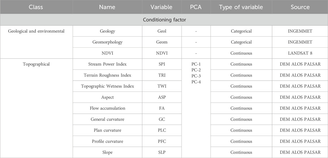
Table 1. Variables for research.

2.3 Methods

The methodology was divided into seven steps (Figure 2). Step 1: It involved collecting geospatial information from national and international institutional repositories. Step 2: The extent of the flooding was determined using multitemporal radar analysis. Step 3: The geospatial information of the conditioning factors was standardized and processed. Step 4: The independence of the topographic factors was determined using Pearson correlation, multicollinearity elimination, and principal component analysis. Step 5: The weight of the conditioning factors in relation to flood occurrence was determined using the frequency ratio and weights of evidence methods. Step 6: The flooding point vectors were divided randomly into flood and non-flood zones in an 80/20 proportion to obtain the training and validation datasets. Additionally, six FSM were constructed, including RF-q, RF-FR, RF-WoE, SVM-q, SVM-FR, and SVM-WoE. Step 7: The performance of each model was analyzed and compared using evaluation metrics such as AUC value, F-1 score, and accuracy. Additionally, overfitting issues were avoided by applying cross-validation. Finally, the contribution of each conditioning factor to the susceptibility model with the best evaluation metrics was determined using SHAP.

Figure 2

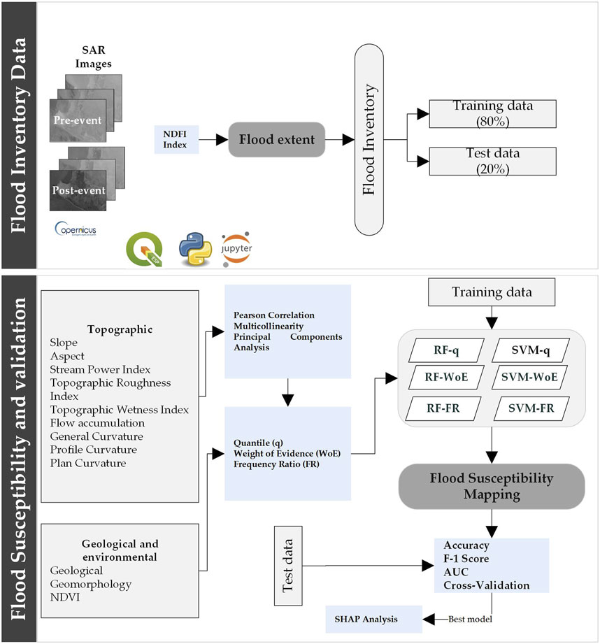
Figure 2. Research flow chart.

2.3.1 Flood extent mapping

To map the extent of flooding during the 2017 Coastal ENSO event, Sentinel-1 radar images were analyzed. These images included two periods: before the rainfall event (July 17 and 27 September 2016) and during the rainfall event (March 20, 23, 26, and April 4). The radar images were downloaded from the Copernicus portal, and preprocessing was carried out, including radiometric and geometric corrections. Additionally, a 3 × 3 adaptive Lee filter was applied to eliminate speckle effects in the images using SNAP software (European Space Agency). Once the radar images were filtered, the Normalized Difference Flood Index (NDFI) was estimated (see Equation 1), aiming to highlight temporal changes in open water areas (Cian et al., 2018a).

$\mathit{N}\mathit{D}\mathit{F}\mathit{I}=\frac{\mathit{m}\mathit{e}\mathit{a}\mathit{n}{\mathit{\vartheta }}_{\mathbf{0}}\left(″\mathit{r}\mathit{e}\mathit{f}\mathit{e}\mathit{r}\mathit{e}\mathit{n}\mathit{c}{\mathit{e}}^{″}\right)-\mathit{min}{\mathit{\vartheta }}_{\mathbf{0}}\left(″\mathit{r}\mathit{e}\mathit{f}\mathit{e}\mathit{r}\mathit{e}\mathit{n}\mathit{c}\mathit{e}+\mathit{f}\mathit{l}\mathit{o}\mathit{o}{\mathit{d}}^{″}\right)}{\mathit{m}\mathit{e}\mathit{a}\mathit{n}{\mathit{\vartheta }}_{\mathbf{0}}\left(″\mathit{r}\mathit{e}\mathit{f}\mathit{e}\mathit{r}\mathit{e}\mathit{n}\mathit{c}{\mathit{e}}^{″}\right)+\mathit{min}{\mathit{\vartheta }}_{\mathbf{0}}\left(″\mathit{r}\mathit{e}\mathit{f}\mathit{e}\mathit{r}\mathit{e}\mathit{n}\mathit{c}\mathit{e}+\mathit{f}\mathit{l}\mathit{o}\mathit{o}{\mathit{d}}^{″}\right)}(1)$

Where $mean{\vartheta }_0\left(″{\text{reference}}^{″}\right)$ is the average pixel value of the pre-event raster, and $\mathit{min}{\vartheta }_0\left(″\text{reference}+{\text{flood}}^{″}\right)$ represents the minimum values of the maximum flood images, i.e., during the rainy stage. The threshold value for distinguishing flooded areas from non-flooded areas was established using an empirical approach set by (Cian et al., 2018a), which for the purposes of this study was set to 0.35. Finally, two additional filters were applied, which included removing all pixels smaller than 100 m and flooded areas located on slopes greater than 5°.

2.3.2 Flood susceptibility mapping (FSM)

Flood susceptibility is defined as the probability of a flood occurring in a given area based on the local physical conditions that determine its predisposition (Vojtek and Vojteková, 2019; Hao et al., 2021). FSM is a crucial tool for identifying areas prone to flooding, land-use planning, preparedness (Kaya and Derin, 2023), and for reducing and reconstruction in emergency or disaster situations. Additionally, 10 variables were selected from previous studies (Khosravi et al., 2019; Gudiyangada Nachappa et al., 2020; Kaya and Derin, 2023; Maharjan et al., 2024), including topographic, hydrological, geological, and environmental variables as independent variables for the models, which are detailed in Table 1. The topographic and hydrological variables were derived from the Copernicus Digital Elevation Model with a spatial resolution of 30 m. Furthermore, the NDVI was processed using Landsat-8 images from March 2017, applying Equation 2, and downloaded from the Google Earth Engine platform. All additional variables were obtained from repositories of technical and scientific institutions and rasterized to the same spatial resolution of 30 m.

$\mathit{N}\mathit{D}\mathit{V}\mathit{I}=\frac{\mathit{n}\mathit{e}\mathit{a}\mathit{r}\mathit{i}\mathit{n}\mathit{f}\mathit{r}\mathit{a}\mathit{r}\mathit{e}\mathit{d}-\mathit{r}\mathit{e}\mathit{d}}{\mathit{n}\mathit{e}\mathit{a}\mathit{r}\mathit{i}\mathit{n}\mathit{f}\mathit{r}\mathit{a}\mathit{r}\mathit{e}\mathit{d}+\mathit{r}\mathit{e}\mathit{d}}(2)$

2.3.3 Positive and negative flood samples

The positive flood sample layer, in point format, used for training and evaluating the flood susceptibility mapping, was digitized based on the flood extent from Step 2. The points were randomly extracted from the centroid of the flood polygons, ensuring full coverage of the study area. On the other hand, the digitization of negative samples was done under two criteria: first, by digitizing negative samples in areas of very low, low, and medium flood susceptibility based on a prior heuristic susceptibility model developed by INGEMMET. Additionally, since floods do not occur in high-elevation and slope areas such as hillside zones, these were randomly digitized, ensuring that a large portion of the study area was covered. This hybrid approach for negative samples improves the performance and reliability of the models (Khabiri et al., 2023). It is important to note that a total of 182 positive and negative samples were used, with an equal proportion between them, and 80% of the data was used for training and 20% for model evaluation. Although the sample size may appear limited, it reflects the absence of a detailed flood inventory in the region (only 58 events officially reported by INGEMMET as of 2025) and remains consistent with watershed-scale studies employing similar sample sizes (Rahmati et al., 2016; Khosravi et al., 2019; Yariyan et al., 2020; Singha et al., 2022).

2.3.4 Exploratory method of variables

In this study, both simple and hybrid quantitative flood susceptibility mapping were compared using bivariate statistical techniques and ML methods. Simple models of RF-q and SVM-q were constructed, along with two hybrid models combining RF with FR (RF-FR) and WoE (RF-WoE); and SVM with FR (SVM-FR) and WoE (SVM-WoE). Prior to including the variables in the models, an exploratory variable analysis was conducted to ensure the linear independence of each topographic variable derived from the DEM, to reduce noise and enhance the predictive capability of the models (Hu et al., 2020). To ensure independence and avoid relationships between two or more independent variables in the models, a Pearson correlation analysis was performed, and multicollinearity was discarded (Chan et al., 2022) using the variance inflation factor (VIF). Pearson correlation values higher than ±0.8 and VIF values greater than five or 10 indicate issues of interrelationship and multicollinearity between topographic variables (Menard, 2002; Field, 2009). To address this problem, Principal Component Analysis (PCA) was applied, with the primary goal of ensuring independence and reducing the number of variables into a set of mutually independent principal components (Kelkar, 2017) without the need to eliminate variables (Badillo-Rivera et al., 2024). The number of principal components that summarize the original data was established based on the cumulative variance explanation threshold, which ranges from 0 to 1. For this study, a minimum value of 0.6 was used, similar to previous studies (Goyes-Peñafiel and Hernandez-Rojas, 2021; Ahmed et al., 2023; Badillo-Rivera et al., 2024). Once the dimensionality of the topographic variables was reduced and the geological and environmental variables were standardized to the same format and spatial resolution, the quantitative relationship or true weight between each class of the conditioning factors (independent variables) and flood occurrence (dependent variable) was estimated using bivariate statistical techniques, FR, and WoE.

2.3.5 Statistical models

2.3.5.1 Frequency ratio (FR)

Regarding FR, it refers to the relationship between the percentage of flooded area for each class of each conditioning factor and the percentage of the area of that specific class (Tehrany and Kumar, 2018). Equation 3 was used to calculate the FR value for each class of each conditioning factor (Dey et al., 2024).

${\mathit{F}\mathit{R}}_{\mathit{i}}=\frac{\frac{\mathit{F}\mathit{p}\mathit{i}\mathit{x}\mathit{i}}{{\displaystyle {\sum }_{\mathit{i}=\mathbf{1}}^{\mathit{n}}}\mathit{F}\mathit{p}\mathit{i}\mathit{x}\mathit{i}}}{\frac{\mathit{T}\mathit{p}\mathit{i}\mathit{x}\mathit{i}}{{\displaystyle {\sum }_{\mathit{i}=\mathbf{1}}^{\mathit{n}}}\mathit{T}\mathit{p}\mathit{i}\mathit{x}\mathit{i}}}(3)$

Where FRi is the frequency ratio value for each class i of each factor of the variable, Fpixi is the number of flooded pixels for each i class, and Tpixi represents the total number of pixels for each i class. Finally, n is the total number of classes for each conditioning factor. Flood susceptibility is equal to the sum of all FR values for each factor, as shown in Equation 4 (Natarajan et al., 2021). FR values greater than one indicate a strong correlation with floods, while values below one indicate a weak correlation (Tehrany and Kumar, 2018).

$\mathit{F}\mathit{S}=\sum \mathit{F}\mathit{R}\mathit{i}(4)$

2.3.5.2 Weight of evidence (WoE)

On the other hand, the WoE is a quantitative, data-driven Bayesian probability model (Bonham-Carter, 1995; Rahmati et al., 2016). Using the flood layer and conditioning factors, WoE was applied to determine the relationship and weight of each relevant factor. The weights for each flood conditioning factor (A) can be calculated by analyzing the spatial relationship between the presence or absence of flooding (B) within a specific area (Bonham-Carter, 1995; Van Westen, 2002; Tehrany et al., 2014b). The method assigns a positive $\left(W_i^{+}\right.$) or negative $\left(W_i^{-}\right.$) weight to each class of the conditioning factor based on the degree of association between the class of the factor and the spatial distribution and density of flood evidence (Badillo-Rivera et al., 2024). If $W_i^{+}$ is positive (see Equation 5), it indicates that the presence of the causative factor is favorable for the occurrence of flooding, and the magnitude of this weight indicates the positive correlation between the presence of the causative factor and flooding. If $W_i^{+}$ is negative, it is not favorable. On the other hand, $W_i^{-}$ is used to assess the importance of the absence of the conditioning factor for the occurrence of flooding. If $W_i^{-}$ is positive (see Equation 6), the absence of the conditioning factor is favorable for flooding occurrence, and when it is negative, it is not, with the magnitude indicating the level of negative correlation (Van Westen, 2002; Meten and Bhandary, 2020).

${\mathit{W}\mathit{i}}^{+}=\mathbf{ln}\left(\mathit{P}\left(\mathit{A}|\mathit{B}\right)/\mathit{P}\left(\mathit{A}|\overline{\mathit{B}}\right)\right)(5)$

${\mathit{W}\mathit{i}}^{-}=\mathbf{ln}\left(\mathit{P}\left(\overline{\mathit{A}}|\mathit{B}\right)/\mathit{P}\left(\overline{\mathit{A}}|\overline{\mathit{B}}\right)\right)(6)$

Where P is the probability, ln is the natural logarithm, A and $\overline{A}$ represent the presence and absence of the conditioning factor, respectively, and B and $\overline{B}$ represent the presence and absence of flooding. The difference between ${Wi}^{+}$ and ${Wi}^{-}$ is known as the contrast factor (Bhandari et al., 2024), and it reveals the spatial association between the conditioning factor. A positive value indicates a positive relationship, while a negative value indicates a negative or unfavorable relationship for the occurrence of flooding (Van Westen, 2002; Gentilucci et al., 2023).

2.3.6 Machine learning models

2.3.6.1 Random forest (RF)

The RF algorithm is a combination of predictive trees such that each tree depends on the values of a random vector sampled independently and with the same distribution for all the trees in the forest (Breiman, 2001). The model, proposed by Breiman, combines the theory of Bagging, which refers to bootstrap aggregation (Murphy and Murphy, 2012), random split selection, and the random feature selection process (Sharafat et al., 2024). RF can be used in regression and classification problems using a majority voting scheme (Bhattacharya, 2021), and it has the capability to predict dependent variables using independent variables. Additionally, unlike linear modeling tools, RF is a nonlinear tool that can handle multivariate prediction problems and is not sensitive to outliers. Therefore, RF models achieve high accuracy in classification by reducing overfitting errors reported in models (Farhadi and Najafzadeh, 2021; Ghosh and Dey, 2021; Li et al., 2023; Liao et al., 2024; Sharafat et al., 2024). Equation 7 represents the RF algorithm.

${\widehat{\mathit{C}}}_{\mathit{r}\mathit{f}}=\mathit{m}\mathit{a}\mathit{j}\mathit{o}\mathit{r}\mathit{i}\mathit{t}\mathit{y}\mathit{v}\mathit{o}\mathit{t}\mathit{e}\{{\left.{\widehat{\mathit{C}}}_{\mathit{n}}\left(\mathit{x}\right)\right\}}_{\mathit{n}=\mathbf{1}}^{\mathit{N}}(7)$

Where ${\widehat{C}}_{rf}$ is the final predicted class of RF, ${\widehat{C}}_n$ is the predicted class for the nth decision tree in a forest for the observation (x), and N indicates the number of decision trees in the forest (Nurwatik et al., 2022).

2.3.6.2 Support vector machine (SVM)

On the other hand, SVM is a supervised ML method capable of solving classification and regression problems, as proposed by (Cortes and Vapnik, 1995). It is based on class discrimination in a high-dimensional feature space generated through nonlinear transformations of the predictors. For two-class classification problems, SVM aims to find an optimal separating plane, known as a hyperplane in the feature space, which maximizes the separation between the two classes of samples (Merghadi et al., 2020; Li et al., 2023). Consider a matrix of conditioning factors, X = (X1, X2, Xn); Yj = (Y1, Y2) is a vector of non-flooding and flooding classes, and the optimal hyperplane can be obtained by solving the classification function as follows (see Equation 8).

$\mathit{f}\left(\mathit{X}\right)=\mathit{s}\mathit{i}\mathit{g}\mathit{n}\left[{\displaystyle \sum _{\mathit{i}=\mathbf{1}}^{\mathit{n}}}{\mathit{\alpha }}_{\mathit{i}}{\mathit{Y}}_{\mathit{j}}\mathit{k}\left(\mathit{X},{\mathit{X}}_{\mathit{i}}\right)+\mathit{c}\right](8)$

Where c is the offset from the origin of the hyperplane, n is the number of flood conditioning factors, ${\alpha }_i$ is a positive real constant, and $k\left(X,X_i\right)$ is the kernel function, which can be linear, polynomial, radial basis or sigmoidal (Pham et al., 2016). The solution can be further reviewed in (Zhang et al., 2021). In this study, the Python scikit-learn module was applied to implement the RF and SVM models. It is worth mentioning that the hybrid RF and SVM models with FR and WoE were modeled based on the weights assigned to each conditioning factor class derived from Step 5.

In this study, hyperparameters for RF and SVM were adopted from commonly used configurations reported in the literature, as an exhaustive optimization was not the focus, as highlighted by Liu et al. (2023b), many ML models achieve robust accuracy with default parameters, and exploring all possible hyperparameter combinations is computationally impractical. Table A1 presents the hyperparameters used for SVM and RF.

2.3.6.3 Shapely additive exPlanations (SHAP)

The construction of FSM based on ML techniques has been improved using hybrid approaches, as demonstrated in (Tehrany et al., 2014b; Gudiyangada Nachappa et al., 2020; Towfiqul Islam et al., 2021). However, stakeholders do not widely use these models despite their higher accuracy compared to traditional models, due to their black-box nature (Pradhan et al., 2023). In this research, the SHAP technique was incorporated to quantify the degree of influence of each conditioning factor in the FSM that presented the best evaluation metrics. This was done in order to create a more interpretable and transparent machine learning model to explain the black-box model (Aksoy et al., 2024; Tripathi and Prakash, 2024). SHAP is a technique introduced by (Lundberg and Lee, 2017) that is based on game theory to estimate the importance of each player in relation to their contributions in a coalition game (Tripathi and Prakash, 2024). For each predicted sample, the SHAP technique generates a value, which is the sum of the values assigned to each feature (see Equation 9) (Wang et al., 2023).

$\mathit{g}\left(\acute{\mathit{z}}\right)={\varnothing }_{\mathbf{0}}+{\displaystyle \sum _{\mathit{j}=\mathbf{1}}^{\mathit{M}}}{\varnothing }_{\mathit{j}}{\acute{\mathit{z}}}_{\mathit{j}}(9)$

Where g is each variable, $\acute{z}$ is the explanation model ∈ {0, 1}M, is the number of simplified input features, and ${\varnothing }_j$ ∈ ℝ, is the attribution of the feature for feature j, which represents the Shapley value. A deeper explanation can be found in (Lundberg and Lee, 2017).

2.3.7 Evaluation metrics

The receiver operating characteristic curve (ROC) is widely used in geosciences (Rahmati et al., 2016; Khosravi et al., 2019). It can be constructed by plotting specificity (false positive rate, FPR, Equation 10) on the X-axis and sensitivity (true positive rate, TPR, Equation 11) on the Y-axis (Towfiqul Islam et al., 2021). The area under the curve (AUC, Equation 12) of the ROC curve indicates the accuracy in predicting flooded and non-flooded areas and is a useful tool for measuring discriminatory power, evaluating, and quantitatively comparing several models (Gudiyangada Nachappa et al., 2020). It is also the most commonly applied criterion for determining the most suitable model for susceptibility mapping (Sun et al., 2018). FSMs can be evaluated qualitatively based on their accuracy and predictive capacity, as follows: a poor model for AUC values between 0.5 and 0.6, an average model with AUC values between 0.6 and 0.7, a good model for AUC values between 0.7 and 0.8, a very good model for AUC values between 0.8 and 0.9, and an excellent model for values above 0.9 (Pourghasemi et al., 2013; Rahmati et al., 2016). On the other hand, evaluation metrics such as accuracy (Equation 13) and F-1 score (Equation 14) have been used to assess the predictive capacity of FSMs.

$\mathit{x}=\mathbf{1}-\mathit{s}\mathit{p}\mathit{e}\mathit{c}\mathit{i}\mathit{f}\mathit{i}\mathit{t}\mathit{y}=\mathit{F}\mathit{P}\mathit{R}=\mathbf{1}-\left(\frac{\mathit{T}\mathit{N}}{\mathit{T}\mathit{N}+\mathit{F}\mathit{P}}\right)(10)$

$\mathit{y}=\mathit{s}\mathit{e}\mathit{n}\mathit{s}\mathit{i}\mathit{t}\mathit{i}\mathit{v}\mathit{i}\mathit{t}\mathit{y}=\mathit{T}\mathit{P}\mathit{R}=\left(\frac{\mathit{T}\mathit{P}}{\mathit{T}\mathit{P}+\mathit{F}\mathit{N}}\right)(11)$

$\mathit{A}\mathit{U}\mathit{C}=\frac{\sum \mathit{T}\mathit{P}+\sum \mathit{T}\mathit{N}}{\mathit{P}+\mathit{N}}(12)$

$\mathit{A}\mathit{c}\mathit{c}\mathit{u}\mathit{r}\mathit{a}\mathit{c}\mathit{y}=\frac{\mathit{T}\mathit{P}+\mathit{T}\mathit{N}}{\mathit{T}\mathit{P}+\mathit{F}\mathit{P}+\mathit{T}\mathit{N}+\mathit{F}\mathit{N}}(13)$

$\mathit{F}-\mathbf{1}\mathit{s}\mathit{c}\mathit{o}\mathit{r}\mathit{e}=\frac{\mathbf{2}\times \mathit{T}\mathit{P}}{\mathbf{2}\times \mathit{T}\mathit{P}+\mathit{F}\mathit{P}+\mathit{F}\mathit{N}}(14)$

Where TN and TP are the true negatives and true positives, respectively, and indicate the number of pixels that were classified correctly; FN and FP are the false negatives and false positives, respectively, and indicate the number of pixels that were classified incorrectly; N and P are the total number of negative and positive samples, respectively (Rahmati et al., 2016; Chen et al., 2018). Accuracy (ACC) indicates the proportion of correct predictions in relation to the total number of predictions made, while the F-1 score represents the model’s performance by combining precision and recall. Higher values of accuracy and F-1 score indicate a better model, with a value of one representing a perfect model (Chen et al., 2018; Pradhan et al., 2021; Li et al., 2023).

2.3.8 Cross validation (CV)

CV is a resampling technique used to assess the robustness of a model prediction and to aid in model selection (Chung and Fabbri, 2008; Friedl and Stampfer, 2012). It is often applied to prevent overfitting, enhance robustness, and ensure stability in ML models (Khosravi et al., 2019; Chen et al., 2020; Liu et al., 2023a). In CV, a subset of the sample is reserved to validate the model performance (Chan et al., 2022). In this study, the data was randomly divided into five equal parts (k = 5 folds) using the scikit-learn module in Python. The ML models were trained and validated k times, and the mean and standard deviation of AUC (AUC-CV), accuracy (ACC-CV), and F-1score (F-1score-CV) were obtained.

3 Results

3.1 Flood extent mapping and flood susceptibility mapping

The spatial distribution of flooded areas due to intense rainfall generated by the 2017 coastal ENSO is shown in Figure 3. The blue-colored surfaces represent the maximum recorded flooding between March 20 and 4 April 2017, covering a total of 1,637.2 km², mainly in areas at or near sea level. These floods affected agricultural, urban, and rural areas. It is important to mention that the flood extent is limited by the availability of Sentinel-1 data for the analyzed flood event.

Figure 3

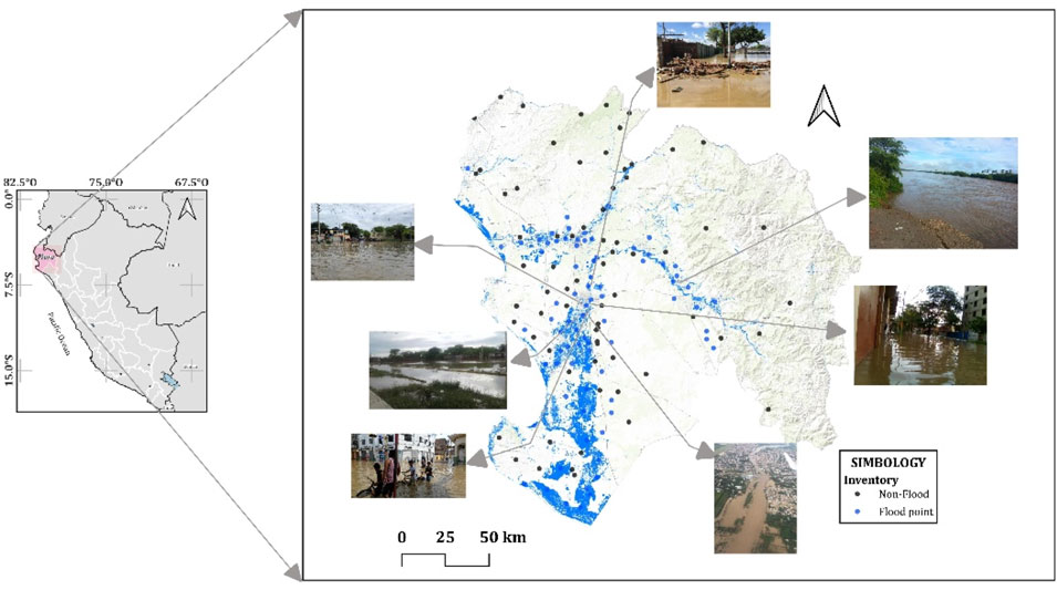
Figure 3. Flood extent. Images from (Miñán-Ubillús and Fahsbender-Céspedes, 2017).

The results of the exploratory analysis of the topographic variables reveal issues of correlation (Figure 4) and multicollinearity (Table 2) between the terrain ruggedness index (TRI) and the slope. The Pearson correlation test confirms a high correlation between these two variables.

Figure 4

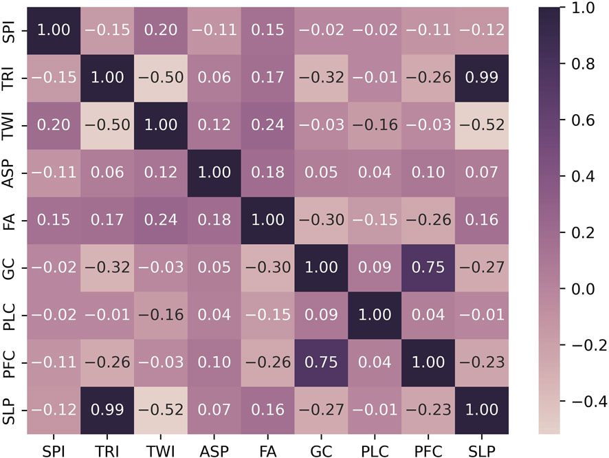
Figure 4. Pearson correlation of topographic variables.

Table 2

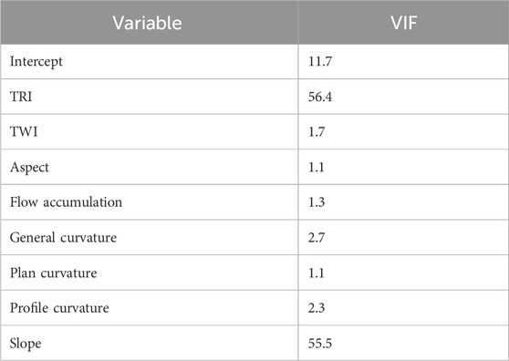
Table 2. Inflation value of the variance of the topographic variables.

Furthermore, in the multicollinearity test, variance inflation factor (VIF) values range from 1.1 (for aspect and plan curvature) to 56.4 (TRI), indicating interrelation and multicollinearity issues between slope and TRI. These VIF values are significantly higher than 5, confirming the presence of multicollinearity among the variables derived from the digital elevation model (DEM).

Given the above, it is recommended to proceed with dimensionality reduction using PCA. This approach aims to eliminate variable correlation and resolve the multicollinearity issue before performing susceptibility mapping. Figure 5 shows the variance contribution of the nine principal components (PC). Assuming a variance explanation level above 0.65, four PC are required, collectively explaining 75.4% of the variance. Each of these components is independent, ensuring the elimination of correlation and multicollinearity.

Figure 5

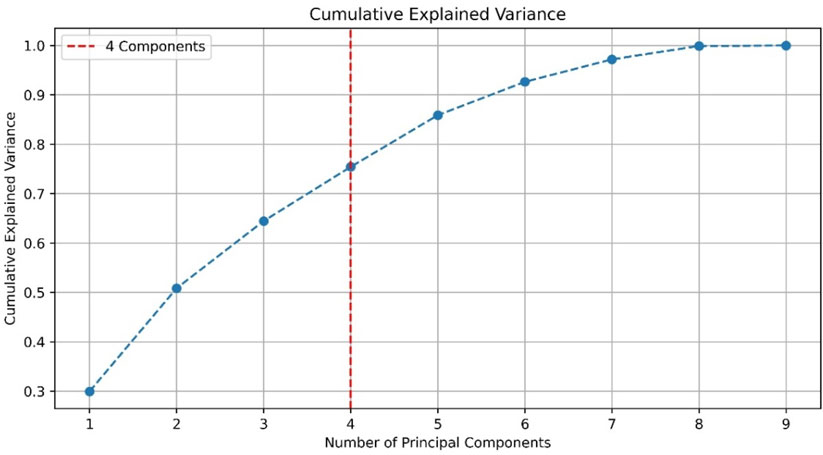
Figure 5. Explanation of the variance of the principal components.

Table 3 presents the importance and contribution of each influential variable in the four PC. The higher the absolute value, the greater the contribution to the PC.

Table 3

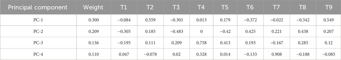
Table 3. Weights of topographic variables in the principal components.

Finally, the four PC (Figure 6) and the NDVI were reclassified into quintiles to be included in the FSM.

Figure 6

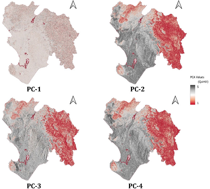
Figure 6. Reclassified principal components with quintiles.

The FSM were generated using ensemble models of SVM and RF. Three main approaches were developed:

First model: Seven variables (PC-1, PC-2, PC-3, PC-4, NDVI, Geology, and Geomorphology) were used for both SVM and RF. This approach generated the initial flood susceptibility maps without considering the relative weight evidenced in flood occurrence.

Second model: The quantitative relationship between the variables and flood occurrence was estimated using the FR technique. The new variables obtained from this analysis were used to generate FSM, namely, SVM-FR and RF-FR.

Third model: A second method was applied to estimate the quantitative relationship between the variables and flood occurrence, known as WoE. With these new variables, the FSM were modeled, namely, SVM-WoE and RF-WoE.

In total, six FSM models were generated, combining the two algorithms (SVM and RF) with the three approaches described earlier. The results of the FSM (Figure 7), expressed as flood probability, ranged from 0 to one for all models. Based on these values, susceptibility was reclassified into five levels: very low, low, medium, high, and very high, using equal intervals. This reclassification allows for a better identification of areas with higher flood susceptibility. The spatial distribution of flood susceptibility levels is illustrated in Figure 7. Areas with high and very high susceptibility are primarily located along rivers, streams, and areas with low slopes. On the other hand, higher slope areas, such as hills and mountains, correspond to low susceptibility areas.

Figure 7

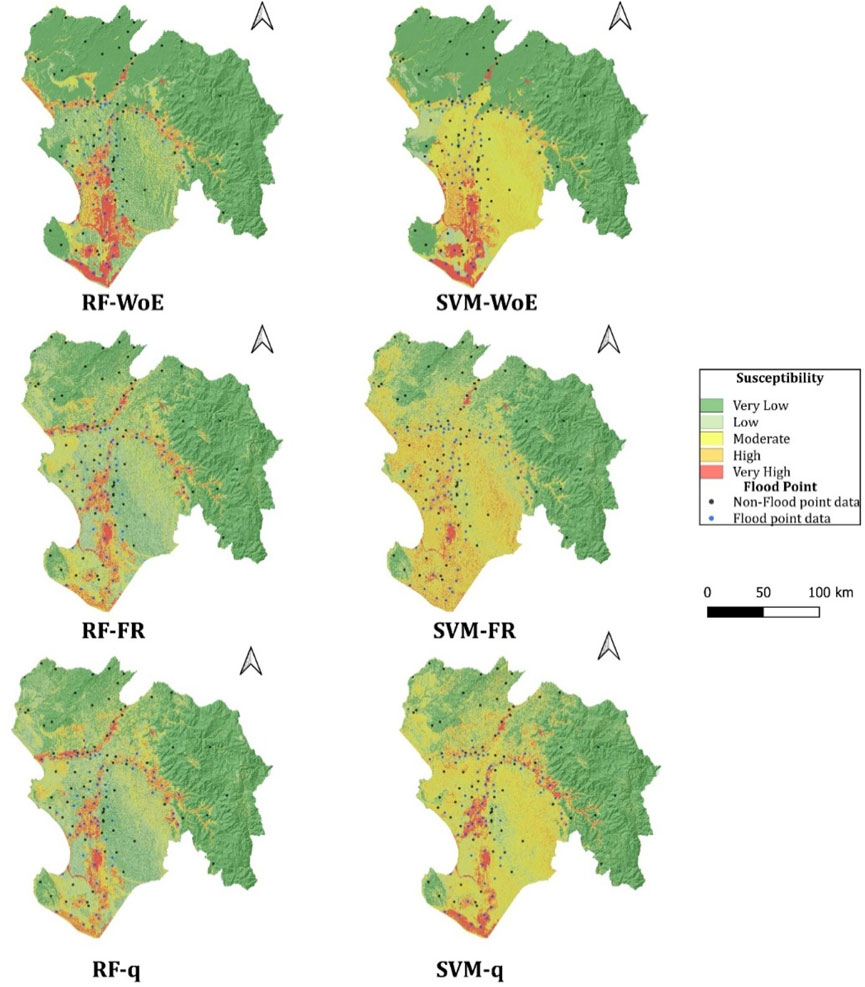
Figure 7. Simple and ensemble flood susceptibility mapping.

Table 4 presents the spatial distribution in terms of area and percentage of the susceptibility levels for all the FSM models.

Table 4

Table 4. Area percentages of susceptibility levels in the flood models.

The area with the highest flood susceptibility level (classified as “very high”) was generated by the RF-WoE model, representing 7.4% of the total area. Following this, in descending order, are the models SVM-q (5.2% of the total area), SVM-WoE (4.6% of the total area), RF-q (4.5% of the total area), and RF-FR (4.4% of the total area). Finally, the most conservative model was the SVM-FR, with only 3.6% of the total area classified as “very high” susceptibility. These results are shown in detail in Figure 8.

Figure 8

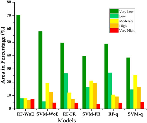
Figure 8. Area expressed as percentages of the different levels of flood susceptibility.

The analyzed models agree that areas close to river courses in the lower basin have a higher probability of flooding, while more distant zones, located in the middle and upper basin, exhibit a lower flood risk. Areas classified with high and very high susceptibility levels are particularly vulnerable to flooding, mainly due to the influence of the Piura River. This river carries a high sediment load and generates significant runoff during events associated with the El Niño phenomenon, particularly in the lower basin. In this area, complex issues related to changes in river morphology are observed, such as the presence of levees, groynes, and sedimented floodplains. Additionally, inadequate land use exacerbates the situation, increasing vulnerability and the risk of recurrent floods. These conditions make the lower basin especially prone to repetitive flooding events (IAHR, 2020). To complement the interpretation of flood susceptibility in relation to urban settlements, the RF–WoE FSM results were overlaid with a geospatial layer of urban and rural population centers in the Piura department. This analysis identified 19 urban and rural settlements, 21,264 population, and 6524 households located within areas classified as very high flood susceptibility. Although the DEM used in this study (30 m resolution) does not explicitly represent urban structures, this approach provides an indirect assessment of urban exposure to flood hazards in the study area.

3.2 Evaluation metrics

Validation criteria were applied to assess the accuracy and effectiveness of the six FSM, during the training phase and the evaluation phase. For this purpose, the AUC value was used; the closer the AUC value is to one, the better the model performance for flood prediction. The training results show that all FSM models reached AUC values greater than 0.850 (Figure 9A). The ensemble model RF-WoE stood out particularly, achieving an AUC = 0.988, outperforming all other models analyzed in the study. Regarding the validation dataset (Figure 9B), it was observed that all models performed well in classifying the presence and absence of floods, with AUC values >0.800. Finally, it was evident that, in both the training and evaluation datasets, the RF-based models, both in their simple and ensemble versions, demonstrated better performance compared to the simple and ensemble SVM models.

Figure 9

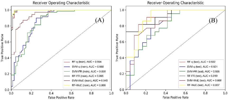
Figure 9. ROC curve and AUC values for the training data (A) and evaluation data (B). The dashed black line represents the no-discrimination line.

A CV analysis was conducted (Table 5) to mitigate overfitting and reduce variability in the models. The CV was calculated as the average of the values obtained from five partitions (k-folds) to facilitate comparison between the different datasets. The AUC-CV values obtained were high in all cases, ranging from 0.828 for the SVM-q model to 0.936 for RF-WoE. Regarding the F1-score-CV and Accuracy-CV metrics, the values ranged from 0.757 (SVM-FR) to 0.851 (RF-WoE) for the former, while accuracy (Accuracy-CV) varied from 0.728 (SVM-FR) to 0.848 (RF-WoE).

Table 5

Table 5. Evaluation metrics for FSM.

The evaluation and CV metrics applied to the models showed that the RF-WoE hybrid model achieved the best performance compared to the SVM model in all its hybrid combinations, and it is the most stable model for zoning flood-prone areas in the study area, as shown in Figure 10.

Figure 10

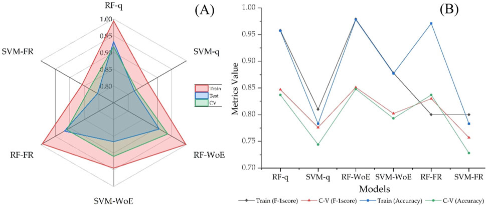
Figure 10. AUC value for the training, testing, and CV data (A), F1-score and accuracy values for training and CV (B).

Figures 11A,B present the variable importance analysis and the influence of features on the RF-WoE model using the SHAP technique on the training dataset. This model was selected due to its superior performance in terms of AUC, F1-score, and accuracy. In Figure 11A, the variable importance ranking is shown. The Y-axis (ordinate) displays the most relevant features for model prediction in descending order, while the X-axis (abscissa) represents the impact of each variable on the prediction. Additionally, the color of the points indicates the intensity of the feature value for each data point. The results indicate that the most influential variable in the FSM prediction is geology, followed by geomorphology and PC-3. In contrast, PC1 and NDVI show values close to zero or have a slightly positive or negative impact on the predictions. On the other hand, Figures 11B,C illustrate the contribution of each variable to the prediction of a specific observation. Higher scores lead the model to predict a value of 1 (greater flood susceptibility), while lower scores result in a prediction of 0 (lower susceptibility). The size of the blue bars represents features that decrease the likelihood of flooding, while the red bars indicate variables that increase this likelihood. Specifically, low values of PC-3, geology, PC-2, and geomorphology push the models prediction towards a score of 0.03 (Figure 11B), suggesting low flood susceptibility. In contrast, high values of geology, geomorphology, PC-2, PC-3, and PC-4 increase the models score up to 0.92, indicating high susceptibility for a specific observation.

Figure 11

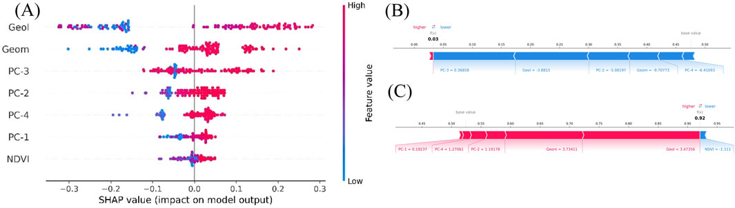
Figure 11. (A), SHAP summary plot; (B,C) SHAP individual force plot.

4 Discussion

FSM play a key role in decision-making related to land-use planning, as they help identify flood-prone areas and reduce economic losses and risks to human life. Zoning and land-use management, supported by appropriate tools and technologies, are essential for reducing flood risks, protecting the environment, and safeguarding vulnerable communities. The main objective of this study was to generate FSM for the Piura region in northern Peru by integrating optical and radar RS data with GIS-based analysis. To address dimensionality and multicollinearity among variables, PCA was applied, enabling the selection of key factors, which proved effective in constructing FSM. ML techniques, specifically RF and SVM, were used to develop six model variants, with a hybrid approach demonstrating improved predictive capability over simpler statistical or single-method approaches (Shahabi et al., 2021; Kaya and Derin, 2023; Badillo-Rivera et al., 2024). However, most machine learning-based susceptibility models still function as black boxes, offering limited interpretability for decision-making. To address this, this study incorporates explainable AI techniques, particularly SHAP analysis, alongside SAR-based flood mapping and statistical integration, creating a comprehensive and interpretable modeling framework designed to strengthen flood risk management in ENSO-affected regions.

The spatial distribution of flooded areas observed during the Coastal ENSO 2017 event reveals significant patterns that highlight the vulnerability of certain areas, especially those with elevations near sea level and close to river courses, particularly the lower Piura River basin, where morphological factors and improper land use exacerbate risk. The floods, covering a total of 1,637.2 km², mainly affected agricultural, urban, and rural areas; however, the reliance on Sentinel-1 data limits a full understanding of the phenomenon, suggesting that future research should consider integrating multiple data sources.

The input variables for the susceptibility models, which showed correlation and multicollinearity issues, indicated that applying techniques such as PCA is crucial to reducing dimensionality and improving the accuracy of susceptibility models. Omitting this procedure in flood susceptibility studies, as seen in some research (Tehrany et al., 2014b; Gudiyangada Nachappa et al., 2020; Yariyan et al., 2020), could lead to models where the reliability of the results is questionable (Waleed and Sajjad, 2025). The proper selection of PC is essential, as it allowed explaining 75.4% of the variance using only four PC, which is consistent with similar values reported by (Ahmed et al., 2023; Badillo-Rivera et al., 2024). This approach optimizes the models without losing critical information, mitigates overfitting, and reduces the impact of outliers (Shojaeian et al., 2024). It was highlighted that the variables with the greatest influence on the PC are TRI and slope for PC-1, TWI and profile curvature for PC-2, aspect and flow accumulation for PC-3, and plan curvature for PC-4. The six models analyzed in this study resulted in similar susceptibility distribution patterns, revealing significant differences in the extent of high-susceptibility areas.

The RF-WoE model generated the largest area classified as very high susceptibility, covering 2632.1 km², followed by the SVM-q model with 1,640.4 km². Other models, such as RF-FR, SVM-FR, RF-q, and SVM-WoE, showed a similar distribution in terms of the area classified within the highest susceptibility levels. These results suggest that the RF-WoE model may be more sensitive to very high susceptibility conditions, especially in areas near rivers. Overall, the analyzed models clearly identify the zones with the highest flood susceptibility, located along rivers and in low-slope areas within the lower Piura River basin. These areas are particularly vulnerable during extreme precipitation events, such as those associated with ENSO, which generate high levels of runoff and sedimentation, causing rivers to overflow into flat areas, including floodplains, low and middle terraces, with slopes lower than 5°. Additionally, the anthropogenic modification of the Piura River channel through channelization, bridge construction, and inadequate occupation of vulnerable areas significantly increases the damage during extreme events (Vílchez Mata, 2018). On the other hand, areas with steeper slopes, such as hills and mountainous regions, exhibit lower susceptibility levels since the terrain inclination hinders water accumulation, reducing the likelihood of flooding. However, it is important to note that during extreme events, erosion and sedimentation can pose a risk to lower basins, affecting the dynamics of the fluvial system and exacerbating the impacts of flooding.

The validation of the models in terms of AUC, F-1 score, and accuracy, for both the training and validation datasets, indicates an outstanding performance of the ensemble RF models, particularly the RF-WoE model, which achieved an AUC of 0.988, outperforming the SVM-based models. Although the SVM models show acceptable performance (AUC >0.805 in training, evaluation, and cross-validation), they are inferior compared to RF. This is attributed to the use of a linear kernel in SVM, which limited its ability to capture the nonlinear relationships governing flood susceptibility, a finding consistent with Khodaei et al. (2025). While it is recognized that employing nonlinear kernels (radial basis function (RBF), polynomial) and systematic hyperparameter tuning could potentially enhance SVM performance, studies such as Tehrany et al. (2015) found only a marginal improvement of RBF over a linear kernel in flood susceptibility contexts. This suggests that even after optimization, SVM may not surpass RF in this specific domain. In contrast, RF demonstrated the ability to handle highly complex, nonlinear relationships and exhibited robustness to outliers among input variables (Liao et al., 2024), which contributed to its superior predictive performance. Similar results have been reported in previous studies, such as Plataridis and Mallios, (2023), where the RF-WoE model achieved an AUC of 0.968, outperforming other approaches designed for flood prediction. Additionally, in problems related to landslides and mass movements, RF-WoE models have proven to be the best performing in terms of AUC compared to other models used (Chen et al., 2019; Wei et al., 2023; Badillo-Rivera et al., 2024). The CV analysis supports the robustness of the models, with AUC-CV values ranging from 0.828 to 0.936, suggesting that the models are not overfitted and demonstrate good overall performance in different scenarios (Goetz et al., 2015; Chen et al., 2018).

SHAP values help validate the model by confirming that the most influential features align with factors associated with flooding, such as geology (alluvial, fluvial, eolian, lacustrine deposits, among others); geomorphology (floodplains, alluvial plains, depression reliefs, alluvial terraces, estuaries, dune fields, etc.), where higher probability values for flooding are associated with flat surfaces; and aspect, which is the variable with the greatest influence on PC3, indicating the direction of maximum slope and being related to the direction of water flow, pointing to flat areas (Seleem et al., 2022) prone to flooding. According to the force plot in Figures 11B,C, low values, mainly from geology and geomorphology, significantly push the prediction towards no floods in the RF-WoE model output, while high values of these same variables reveal the opposite, meaning they strongly influence the model to predict floods. This demonstrates their critical relevance in the decision-making process within the model.

The spatial distribution of flooding during the 2017 Coastal ENSO may be limited by the availability and quality of Sentinel-1 data, which restricts the ability to capture all flooding events due to limited temporal resolution and availability. It is therefore recommended to integrate multiple data sources to improve the understanding of the flooding phenomenon. The developed FSMs are specific to the northern region of Peru, particularly Piura, which may limit their applicability to other regions with different geographical and climatic characteristics. Additionally, the study focuses on floods associated with the 2017 Coastal ENSO event, and other extreme events or climatic conditions were not considered. The models may not represent other areas that could be affected, although a visual validation was performed with the flood footprint from other extreme events, such as the 1983/84 and 1997/98 ENSO events. A large portion of the flood footprint coincides with the findings reported in this study for 2017. Future studies should integrate multiple data sources, such as LiDAR and high-resolution optical imagery, to improve the accuracy and temporal resolution of flood mapping. Furthermore, no transformation pre-treatments were applied in this study to force a normal distribution in the data, given their topographic nature and the risk of distorting the original information, as reported by Reid and Spencer (2009). Future studies are encouraged to explore the impact of different normalization techniques through sensitivity analyses to evaluate their effect on the stability of principal components and derived susceptibility models.

5 Conclusion

This study demonstrated that combining optical and radar RS with GIS and ML techniques significantly improves flood susceptibility mapping, offering a robust framework for risk assessment and land-use planning in flood-prone areas. The application of PCA was crucial to address multicollinearity issues and improve the accuracy of the models. Areas near rivers and surfaces with low slopes showed the highest susceptibility, confirming the importance of morphological configuration and land use in the occurrence of flooding. By integrating SAR-derived flood mapping with a hybrid modeling approach (RF and SVM combined with statistical techniques), this research provides a novel, transparent, and replicable methodology for regions affected by ENSO-driven floods, where cloud cover and data scarcity have historically limited reliable mapping. The ensemble RF-WoE model proved to be the most effective in predicting flood susceptibility in northern Peru, Piura, achieving AUC values greater than 0.9 for training, evaluation, and cross-validation data, indicating a high level of accuracy. The use of SHAP analysis further strengthened the interpretability of the models by validating that geological, geomorphological, and DEM-derived variables, such as aspect, play a dominant role in flood prediction, making the model outputs more transparent and actionable for decision-makers. This aligns with the understanding that flood processes, configuration, and surface deposit types play a crucial role in water accumulation and flow.

Overall, this study demonstrates the value of combining explainable AI, ML, and RS to develop robust tools for disaster risk reduction, bridging a critical gap in flood susceptibility studies in ENSO-affected areas. It is essential to conduct further research that integrates multiple data sources and diverse hydrometeorological events to improve the generalization and applicability of the models at regional and national levels. The generated models provide valuable information for land zoning and the planning of both gray and green infrastructure, aiming to minimize flood risks and protect vulnerable populations.

Data availability statement

The datasets presented in this study can be found in online repositories. The names of the repository/repositories and accession number(s) can be found in the article/supplementary material.

Author contributions

EB-R: Visualization, Resources, Funding acquisition, Project administration, Writing – original draft, Validation, Formal Analysis, Writing – review and editing, Conceptualization, Supervision, Data curation, Investigation, Software, Methodology. RS: Formal Analysis, Validation, Data curation, Writing – review and editing. IP: Validation, Formal Analysis, Visualization, Writing – review and editing. TC: Formal Analysis, Writing – review and editing, Conceptualization, Validation. AA-P: Validation, Writing – review and editing. AA-A: Validation, Writing – review and editing. EH: Validation, Writing – review and editing. ES: Writing – review and editing, Validation. LE: Validation, Writing – review and editing. HL: Writing – review and editing, Validation. PV-V: Validation, Writing – review and editing.

Funding

The author(s) declare that no financial support was received for the research and/or publication of this article.

Acknowledgments

The authors are grateful to the reviewers for their insightful remarks for enlightening the manuscript.

Conflict of interest

The authors declare that the research was conducted in the absence of any commercial or financial relationships that could be construed as a potential conflict of interest.

Generative AI statement

The author(s) declare that no Generative AI was used in the creation of this manuscript.

Any alternative text (alt text) provided alongside figures in this article has been generated by Frontiers with the support of artificial intelligence and reasonable efforts have been made to ensure accuracy, including review by the authors wherever possible. If you identify any issues, please contact us.

Publisher’s note

All claims expressed in this article are solely those of the authors and do not necessarily represent those of their affiliated organizations, or those of the publisher, the editors and the reviewers. Any product that may be evaluated in this article, or claim that may be made by its manufacturer, is not guaranteed or endorsed by the publisher.

References

Afshari, S., Tavakoly, A. A., Rajib, M. A., Zheng, X., Follum, M. L., Omranian, E., et al. (2018). Comparison of new generation low-complexity flood inundation mapping tools with a hydrodynamic model. J. Hydrol. 556, 539–556. doi:10.1016/j.jhydrol.2017.11.036

CrossRef Full Text | Google Scholar

Ahmed, A., Al Maliki, A., Hashim, B., Alshamsi, D., Arman, H., and Gad, A. (2023). Flood susceptibility mapping utilizing the integration of geospatial and multivariate statistical analysis, erbil area in Northern Iraq as a case study. Sci. Rep. 13, 11919–13. doi:10.1038/s41598-023-39290-4

PubMed Abstract | CrossRef Full Text | Google Scholar

Aksoy, S., Sertel, E., Roscher, R., Tanik, A., and Hamzehpour, N. (2024). Assessment of soil salinity using explainable machine learning methods and Landsat 8 images. Int. J. Appl. Earth Obs. Geoinf. 130, 103879. doi:10.1016/j.jag.2024.103879

CrossRef Full Text | Google Scholar

Al-Aizari, A. R., Al-Masnay, Y. A., Aydda, A., Zhang, J., Ullah, K., Islam, A. R. M. T., et al. (2022). Assessment analysis of flood susceptibility in tropical desert area: a case Study of Yemen. Remote Sens. 14, 4050. doi:10.3390/rs14164050

CrossRef Full Text | Google Scholar

Badillo-Rivera, E., Olcese, M., Santiago, R., Muñoz, N., Rojas-le, C., Ch, T., et al. (2024). A comparative Study of susceptibility and hazard for mass movements applying quantitative machine learning techniques — case Study: northern Lima commonwealth, Peru. Geosciences 14, 168. doi:10.3390/geosciences14060168

CrossRef Full Text | Google Scholar

Benoudjit, A. (2020). Operational mapping of the flood extent and depth from SAR images. University of Surrey. Available online at: https://openresearch.surrey.ac.uk/esploro/outputs/doctoral/Operational-mapping-of-the-flood-extent/99515315702346.

Google Scholar

Bentivoglio, R., Isufi, E., Jonkman, S. N., and Taormina, R. (2022). Deep learning methods for flood mapping: a review of existing applications and future research directions. Hydrol. Earth Syst. Sci. 26, 4345–4378. doi:10.5194/hess-26-4345-2022

CrossRef Full Text | Google Scholar

Bhandari, B. P., Dhakal, S., and Tsou, C. Y. (2024). Assessing the prediction accuracy of frequency ratio, weight of evidence, Shannon Entropy, and information value methods for landslide susceptibility in the siwalik hills of Nepal. Sustain 16, 2092. doi:10.3390/su16052092

CrossRef Full Text | Google Scholar

Bhattacharya, S. (2021). A primer on machine learning in subsurface geosciences. Austin, USA: Springer.

Google Scholar

Bonham-Carter, G. (1995). Geographic information systems for geoscientists: modelling with GIS. 1st ed. Pergamon. doi:10.1016/0098-3004(95)90019-5

CrossRef Full Text | Google Scholar

Breiman, L. (2001). Random forests. Mach. Learn. 45, 5–32. doi:10.1023/A:1010933404324

CrossRef Full Text | Google Scholar

Brill, F. A. (2022). Applications of machine learning and open geospatial data in flood risk modelling. University of Potsdam. Available online at: https://publishup.uni-potsdam.de/frontdoor/index/index/docId/55594.

Google Scholar

Chan, J. Y.Le, Leow, S. M. H., Bea, K. T., Cheng, W. K., Phoong, S. W., Hong, Z. W., et al. (2022). Mitigating the multicollinearity problem and its machine learning approach: a review. Mathematics 10, 1283. doi:10.3390/math10081283

CrossRef Full Text | Google Scholar

Chen, W., Zhang, S., Li, R., and Shahabi, H. (2018). Performance evaluation of the GIS-based data mining techniques of best-first decision tree, random forest, and naïve Bayes tree for landslide susceptibility modeling. Sci. Total Environ. 644, 1006–1018. doi:10.1016/j.scitotenv.2018.06.389

PubMed Abstract | CrossRef Full Text | Google Scholar

Chen, W., Sun, Z., and Han, J. (2019). Landslide susceptibility modeling using integrated ensemble weights of evidence with logistic regression and random forest models. Appl. Sci. 9, 171. doi:10.3390/app9010171

CrossRef Full Text | Google Scholar

Chen, W., Li, Y., Xue, W., Shahabi, H., Li, S., Hong, H., et al. (2020). Modeling flood susceptibility using data-driven approaches of naïve Bayes tree, alternating decision tree, and random forest methods. Sci. Total Environ. 701, 134979. doi:10.1016/j.scitotenv.2019.134979

PubMed Abstract | CrossRef Full Text | Google Scholar

Chen, Y., Zhang, X., Yang, K., Zeng, S., and Hong, A. (2023). Modeling rules of regional flash flood susceptibility prediction using different machine learning models. Front. Earth Sci. 11, 1117004–1117017. doi:10.3389/feart.2023.1117004

CrossRef Full Text | Google Scholar

Chung, C. J., and Fabbri, A. G. (2008). Predicting landslides for risk analysis - spatial models tested by a cross-validation technique. Geomorphology 94, 438–452. doi:10.1016/j.geomorph.2006.12.036

CrossRef Full Text | Google Scholar

Chowdhury, M. S., Rahman, M. N., Sheikh, M. S., Sayeid, M. A., Mahmud, K. H., and Hafsa, B. (2024). GIS-based landslide susceptibility mapping using logistic regression, random forest and decision and regression tree models in Chattogram District, Bangladesh. Heliyon 10, e23424. doi:10.1016/j.heliyon.2023.e23424

PubMed Abstract | CrossRef Full Text | Google Scholar

Cian, F., Marconcini, M., and Ceccato, P. (2018a). Normalized Difference Flood Index for rapid flood mapping: taking advantage of EO big data. Remote Sens. Environ. 209, 712–730. doi:10.1016/j.rse.2018.03.006

CrossRef Full Text | Google Scholar

Cian, F., Marconcini, M., Ceccato, P., and Giupponi, C. (2018b). Flood depth estimation by means of high-resolution SAR images and lidar data. Nat. Hazards Earth Syst. Sci. 18, 3063–3084. doi:10.5194/nhess-18-3063-2018

CrossRef Full Text | Google Scholar

COMEXPERÚ (2024). Cuál Ha Sido El Impacto Del Fenómeno De El Niño En El Perú? Perspect. FEN, 2024. Available online at: https://www.comexperu.org.pe/articulo/cual-ha-sido-el-impacto-del-fenomeno-de-el-nino-en-el-peru-perspectivas-fen-2024#:∼:text=Asimismo%2Claspérdidaseconómicaspor,fenómenoredujoelcrecimientoesperado (Accessed August 6, 2024).

Google Scholar

CORCUENCAS (2014). Amenazas Y susceptibilidad. Available online at: https://cortolima.gov.co/images/POMCA/Rio_Luisa/IIFase_de_Diagnostico/7.2Amenaza_Susceptibilidad.pdf.

Google Scholar

Cortes, C., and Vapnik, V. (1995). Support-Vector networks. Mach. Learn. 20, 273–297. doi:10.1023/A:1022627411411

CrossRef Full Text | Google Scholar

Coumou, D., and Rahmstorf, S. (2012). A decade of weather extremes. Nat. Clim. Chang. 2, 491–496. doi:10.1038/nclimate1452

CrossRef Full Text | Google Scholar

Dey, H., Shao, W., Moradkhani, H., Keim, B. D., and Peter, B. G. (2024). Urban flood susceptibility mapping using frequency ratio and multiple decision tree-based machine learning models. Nat. Hazards. 120, 10365–10393. doi:10.1007/s11069-024-06609-x

CrossRef Full Text | Google Scholar

Doswell, C. A. (2015). “Hydrology, floods and droughts: flooding”, in Encyclopedia of atmospheric sciences. Second Edition, 201–208. doi:10.1016/B978-0-12-382225-3.00151-1

CrossRef Full Text | Google Scholar

Elkhrachy, I. (2022). Flash flood water depth estimation using SAR images, digital elevation models, and machine learning algorithms. Remote Sens. 14, 440. doi:10.3390/rs14030440

CrossRef Full Text | Google Scholar

EM-DAT (2025). EM-DAT: access data. Available online at: https://public.emdat.be/.

Google Scholar

ENFEN (2017). Informe Técnico Extraordinario N ° 001-2017/ENFEN EL NIÑO COSTERO 2017. Available online at: https://www.dhn.mil.pe/archivos/oceanografia/enfen/nota_tecnica/01-2017.pdf.

Google Scholar

Farhadi, H., and Najafzadeh, M. (2021). Flood risk mapping by remote sensing data and random forest technique. WaterSwitzerl. 13, 3115. doi:10.3390/w13213115

CrossRef Full Text | Google Scholar

Field, A. (2009). Discovering statistics using SPSS. Third Edit. SAGE. Available online at: https://books.google.com.pe/books/about/Discovering_Statistics_Using_SPSS.html?id=IY61Ddqnm6IC&redir_esc=y.

Google Scholar

Friedl, H., and Stampfer, E. (2012). “Cross-Validation”, in Encyclopedia of environmetrics. doi:10.1002/9780470057339.vac062

CrossRef Full Text | Google Scholar

Galarza, E., Kámiche, J., Collado, M., and Pacheco, A. (2012). Impactos del Fenómeno El Niño (FEN) en la economía regional de Piura, Lambayeque y La Libertad. Available online at: http://seguros.riesgoycambioclimatico.org/publicaciones/Informe-Tecnico1.pdf.

Google Scholar

Gentilucci, M., Pelagagge, N., Rossi, A., Domenico, A., and Pambianchi, G. (2023). Landslide susceptibility using climatic–environmental factors using the weight-of-evidence Method—A Study area in central Italy. Appl. Sci. 13, 8617. doi:10.3390/app13158617

CrossRef Full Text | Google Scholar

Gestión (2018). Eventos climáticos como el Niño Costero generan pérdidas cercanas a los US$ 4,800 millones. Available online at: https://gestion.pe/economia/eventos-climaticos-nino-costero-generan-perdidas-cercanas-us-4-800-millones-234209-noticia/(Accessed January 29, 2022).

Google Scholar

Ghosh, A., and Dey, P. (2021). Flood Severity assessment of the coastal tract situated between Muriganga and saptamukhi estuaries of Sundarban delta of India using Frequency Ratio (FR), Fuzzy Logic (FL), Logistic Regression (LR) and Random Forest (RF) models. Reg. Stud. Mar. Sci. 42, 101624. doi:10.1016/j.rsma.2021.101624

CrossRef Full Text | Google Scholar

Goetz, J. N., Brenning, A., Petschko, H., and Leopold, P. (2015). Evaluating machine learning and statistical prediction techniques for landslide susceptibility modeling. Comput. Geosci. 81, 1–11. doi:10.1016/j.cageo.2015.04.007

CrossRef Full Text | Google Scholar

Goyes-Peñafiel, P., and Hernandez-Rojas, A. (2021). Landslide susceptibility index based on the integration of logistic regression and weights of evidence: a case study in Popayan, Colombia. Eng. Geol. 280, 105958. doi:10.1016/j.enggeo.2020.105958

CrossRef Full Text | Google Scholar

Gudiyangada Nachappa, T., Tavakkoli Piralilou, S., Gholamnia, K., Ghorbanzadeh, O., Rahmati, O., and Blaschke, T. (2020). Flood susceptibility mapping with machine learning, multi-criteria decision analysis and ensemble using Dempster Shafer Theory. J. Hydrol. 590, 125275. doi:10.1016/j.jhydrol.2020.125275

CrossRef Full Text | Google Scholar

Hao, C., Yunus, A. P., Siva Subramanian, S., and Avtar, R. (2021). Basin-wide flood depth and exposure mapping from SAR images and machine learning models. J. Environ. Manage. 297, 113367. doi:10.1016/j.jenvman.2021.113367

PubMed Abstract | CrossRef Full Text | Google Scholar

Hu, Q., Zhou, Y., Wang, S., and Wang, F. (2020). Machine learning and fractal theory models for landslide susceptibility mapping: case study from the Jinsha River Basin. Geomorphology 351, 106975. doi:10.1016/j.geomorph.2019.106975

CrossRef Full Text | Google Scholar

IAHR (2020). Particular comprehensive study for the control of floods in Piura River: why was Piura flooded? The phenomenon of degradation (erosion) and aggradation (sedimentation) of Piura river in its upper and lower basin. River Morphol. chang. Available online at: https://www.iahr.org/index/detail/215 (Accessed August 1, 2025).

Google Scholar

INDECI (2017). Compendio Estadístico del INDECI 2017. Available online at: https://www.indeci.gob.pe/wp-content/uploads/2019/01/201802271714541.pdf.

Google Scholar

INGEMMET (2023). Evaluación de zonas críticas por peligros geológicos ante Fenómeno El Niño 2023-2024, en el departamento de Piura. Lima, Perú. Available online at: https://repositorio.ingemmet.gob.pe/handle/20.500.12544/4951.

Google Scholar

IPCC (2021). Clim. Change 2021 Phys. Sci. Basis. Available online at: https://www.ipcc.ch/report/ar6/wg1/.

Google Scholar

Kaya, C. M., and Derin, L. (2023). Parameters and methods used in flood susceptibility mapping: a review. J. Water Clim. Chang. 14, 1935–1960. doi:10.2166/wcc.2023.035

CrossRef Full Text | Google Scholar

Kelkar, K. A. (2017). Mass movement phenomena in the western San Juan mountains, Colorado. Texas A&M University.

Google Scholar

Khabiri, S., Crawford, M. M., Koch, H. J., Haneberg, W. C., and Zhu, Y. (2023). An assessment of negative samples and model structures in landslide susceptibility characterization based on Bayesian network models. Remote Sens. 15, 3200. doi:10.3390/rs15123200

CrossRef Full Text | Google Scholar

Khodaei, H., Nasiri Saleh, F., Nobakht Dalir, A., and Zarei, E. (2025). Future flood susceptibility mapping under climate and land use change. Sci. Rep. 15, 12394–18. doi:10.1038/s41598-025-97008-0

PubMed Abstract | CrossRef Full Text | Google Scholar

Khosravi, K., Shahabi, H., Pham, B. T., Adamowski, J., Shirzadi, A., Pradhan, B., et al. (2019). A comparative assessment of flood susceptibility modeling using Multi-Criteria Decision-Making Analysis and Machine Learning methods. J. Hydrol. 573, 311–323. doi:10.1016/j.jhydrol.2019.03.073

CrossRef Full Text | Google Scholar

Koutsoyiannis, D. (2020). Revisiting the global hydrological cycle: is it intensifying? Hydrol. Earth Syst. Sci. 24, 3899–3932. doi:10.5194/hess-24-3899-2020

CrossRef Full Text | Google Scholar

Kumar, V., Sharma, K. V., Caloiero, T., Mehta, D. J., and Singh, K. (2023). Comprehensive overview of flood modeling approaches: a review of recent advances. Hydrology 10, 141. doi:10.3390/hydrology10070141

CrossRef Full Text | Google Scholar

Li, M., Li, L., Lai, Y., He, L., He, Z., and Wang, Z. (2023). Geological hazard susceptibility analysis based on RF, SVM, and NB models, using the puge section of the Zemu River Valley as an example. Sustain 15, 11228. doi:10.3390/su151411228

CrossRef Full Text | Google Scholar

Liao, M., Wen, H., Yang, L., Wang, G., Xiang, X., and Liang, X. (2024). Improving the model robustness of flood hazard mapping based on hyperparameter optimization of random forest. Expert Syst. Appl. 241, 122682. doi:10.1016/j.eswa.2023.122682

CrossRef Full Text | Google Scholar

Liu, S., Liu, Y., Chu, Z., Yang, K., Wang, G., Zhang, L., et al. (2023a). Evaluation of tropical cyclone disaster loss using machine learning algorithms with an eXplainable artificial intelligence approach. Sustain 15, 12261. doi:10.3390/su151612261

CrossRef Full Text | Google Scholar

Liu, S., Wang, L., Zhang, W., He, Y., and Pijush, S. (2023b). A comprehensive review of machine learning-based methods in landslide susceptibility mapping. Geol. J. 58, 2283–2301. doi:10.1002/gj.4666

CrossRef Full Text | Google Scholar

Lundberg, S. M., and Lee, S. I. (2017). A unified approach to interpreting model predictions. Adv. Neural Inf. Process. Syst. 2017-Decem, 4766–4775. doi:10.48550/arXiv.1705.07874

CrossRef Full Text | Google Scholar

Maharjan, M., Timilsina, S., Ayer, S., Singh, B., Manandhar, B., and Sedhain, A. (2024). Flood susceptibility assessment using machine learning approach in the Mohana-Khutiya River of Nepal. Nat. Hazards Res. 4, 32–45. doi:10.1016/j.nhres.2024.01.001

CrossRef Full Text | Google Scholar

Menard, S. (2002). Applied logistic regression analysis. Colorado, USA: SAGE. doi:10.4135/9781412983433

CrossRef Full Text | Google Scholar

Merghadi, A., Yunus, A. P., Dou, J., Whiteley, J., ThaiPham, B., Bui, D. T., et al. (2020). Machine learning methods for landslide susceptibility studies: a comparative overview of algorithm performance. Earth-Science Rev. 207, 103225. doi:10.1016/j.earscirev.2020.103225

CrossRef Full Text | Google Scholar

Meten, M., and Bhandary, N. P. (2020). Frequency Ratio density, logistic regression and weights of evidence modelling for landslide susceptibility assessment and mapping in yanase and Naka catchments of Southeast shikoku. Japan. doi:10.21203/rs.3.rs-37349/v1

CrossRef Full Text | Google Scholar

Michaelides, S. (2021). Precipitation science: measurement, remote sensing, microphysics and modeling. Amsterdam, Netherlands: Elsevier. doi:10.1016/C2019-0-04124-6

CrossRef Full Text | Google Scholar

Miñán-Ubillús, E., and Fahsbender-Céspedes, J. C. (2017). “Mapa con fotografías georreferenciadas de los daños causados por el Fenómeno del Niño Costero 2017 en Piura”, in I Congreso Internacional de Ingeniería y Dirección de Proyectos III Congreso Regional IPMA – LATNET Universidad de Piura.

Google Scholar

Molleda, P., and Velásquez Serra, G. (2024). El Niño Southern Oscillation and the prevalence of infectious diseases: review. La Granja Rev. Ciencias Vida 40, 9–37. doi:10.17163/lgr.n40.2024.01

CrossRef Full Text | Google Scholar

Murphy., P., and Murphy, K. P. (2012). Machine Learning: a probabilistic perspective. 1st ed. MIT press. Available online at: http://link.springer.com/chapter/10.1007/978-94-011-3532-0_2.

Google Scholar

Natarajan, L., Usha, T., Gowrappan, M., Palpanabhan Kasthuri, B., Moorthy, P., and Chokkalingam, L. (2021). Flood susceptibility analysis in chennai Corporation using frequency ratio model. J. Indian Soc. Remote Sens. 49, 1533–1543. doi:10.1007/s12524-021-01331-8

CrossRef Full Text | Google Scholar

Nurwatik, N., Ummah, M. H., Cahyono, A. B., Darminto, M. R., and Hong, J. H. (2022). A comparison Study of landslide susceptibility spatial modeling using machine learning. ISPRS Int. J. Geo-Information 11, 602. doi:10.3390/ijgi11120602

CrossRef Full Text | Google Scholar

Pascaline, W., and Rowena, B. (2018). Economic losses, poverty and disaster 1998-2017. Available online at: https://www.preventionweb.net/files/61119_credeconomiclosses.pdf.

Google Scholar

Pedzisai, E., Mutanga, O., Odindi, J., and Bangira, T. (2023). A novel change detection and threshold-based ensemble of scenarios pyramid for flood extent mapping using Sentinel-1 data. Heliyon 9, e13332. doi:10.1016/j.heliyon.2023.e13332

PubMed Abstract | CrossRef Full Text | Google Scholar

Pham, B. T., Pradhan, B., Tien Bui, D., Prakash, I., and Dholakia, M. B. (2016). A comparative study of different machine learning methods for landslide susceptibility assessment: a case study of Uttarakhand area (India). Environ. Model. Softw. 84, 240–250. doi:10.1016/j.envsoft.2016.07.005

CrossRef Full Text | Google Scholar

Plataridis, K., and Mallios, Z. (2023). Flood susceptibility mapping using hybrid models optimized with Artificial Bee Colony. J. Hydrol. 624, 129961. doi:10.1016/j.jhydrol.2023.129961

CrossRef Full Text | Google Scholar

Pourghasemi, H. R., Moradi, H. R., and Fatemi Aghda, S. M. (2013). Landslide susceptibility mapping by binary logistic regression, analytical hierarchy process, and statistical index models and assessment of their performances. Nat. Hazards 69, 749–779. doi:10.1007/s11069-013-0728-5

CrossRef Full Text | Google Scholar

Pradhan, B., Sameen, M. I., Al-Najjar, H. A. H., Sheng, D., Alamri, A. M., and Park, H. J. (2021). A meta-learning approach of optimisation for spatial prediction of landslides. Remote Sens. 13, 4521–4530. doi:10.3390/rs13224521

CrossRef Full Text | Google Scholar

Pradhan, B., Lee, S., Dikshit, A., and Kim, H. (2023). Spatial flood susceptibility mapping using an explainable artificial intelligence (XAI) model. Geosci. Front. 14, 101625. doi:10.1016/j.gsf.2023.101625

CrossRef Full Text | Google Scholar

Quinn, W. H., Neal, V. T., and Antunez de Mayolo, S. (1987). El Nino occurrences over the past four and a half centuries. J. Geophys. Res. 92 (14), 14449–14461. doi:10.1029/jc092ic13p14449

CrossRef Full Text | Google Scholar

Rahmati, O., Pourghasemi, H. R., and Zeinivand, H. (2016). Flood susceptibility mapping using frequency ratio and weights-of-evidence models in the Golastan Province, Iran. Geocarto Int. 31, 42–70. doi:10.1080/10106049.2015.1041559

CrossRef Full Text | Google Scholar

Reid, M. K., and Spencer, K. L. (2009). Use of principal components analysis (PCA) on estuarine sediment datasets: the effect of data pre-treatment. Environ. Pollut. 157, 2275–2281. doi:10.1016/j.envpol.2009.03.033

PubMed Abstract | CrossRef Full Text | Google Scholar

Rodriguez De La Cruz, J. A., and Moreno Arqque, M. (2023). Detección y mapeo de inundaciones mediante imágenes SAR, usando el método K-Means Clustering para la evaluación de impactos de desastres ocasionados por el fenómeno El Niño. Caso Cuenca Piura, Región Piura. Univ. Nac. Mayor San Marcos. Available online at: https://hdl.handle.net/20.500.12672/19587.

Google Scholar

Rodríguez-Morata, C., Díaz, H. F., Ballesteros-Canovas, J. A., Rohrer, M., and Stoffel, M. (2019). The anomalous 2017 coastal El Niño event in Peru. Clim. Dyn. 52, 5605–5622. doi:10.1007/s00382-018-4466-y

CrossRef Full Text | Google Scholar

Rozos, E., Dimitriadis, P., and Bellos, V. (2022). Machine learning in assessing the performance of hydrological models. Hydrology, 9, 5–17. doi:10.3390/hydrology9010005

CrossRef Full Text | Google Scholar

Scipión, D., Silva, Y., Kapetas, L., Grace, M., Lim, A., Wall, R., et al. (2018). Building resilience in flood disaster management in northern Peru. Available online at: http://hdl.handle.net/20.500.12816/4751.

Google Scholar

Seleem, O., Ayzel, G., de Souza, A. C. T., Bronstert, A., and Heistermann, M. (2022). Towards urban flood susceptibility mapping using data-driven models in Berlin, Germany. Geomatics, Nat. Hazards Risk 13, 1640–1662. doi:10.1080/19475705.2022.2097131

CrossRef Full Text | Google Scholar

SENAMHI (2014). El fenómeno EL NIÑO en el Perú. Lima, Perú. Available online at: https://www.minam.gob.pe/wp-content/uploads/2014/07/Dossier-El-Niño-Final_web.pdf.

Google Scholar

SENAMHI (2020). Climas del Perú: Mapa de clasificación climática nacional. Available online at: https://www.senamhi.gob.pe/main.php?dp=tumbes&p=mapa-climatico-del-peru.

Google Scholar

Shafizadeh-Moghadam, H., Valavi, R., Shahabi, H., Chapi, K., and Shirzadi, A. (2018). Novel forecasting approaches using combination of machine learning and statistical models for flood susceptibility mapping. J. Environ. Manage. 217, 1–11. doi:10.1016/j.jenvman.2018.03.089

PubMed Abstract | CrossRef Full Text | Google Scholar

Shahabi, H., Shirzadi, A., Ronoud, S., Asadi, S., Pham, B. T., Mansouripour, F., et al. (2021). Flash flood susceptibility mapping using a novel deep learning model based on deep belief network, back propagation and genetic algorithm. Geosci. Front. 12, 101100. doi:10.1016/j.gsf.2020.10.007

CrossRef Full Text | Google Scholar

Shojaeian, A., Shafizadeh-Moghadam, H., Sharafati, A., and Shahabi, H. (2024). Extreme flash flood susceptibility mapping using a novel PCA-based model stacking approach. Adv. Sp. Res. 74, 5371–5382. doi:10.1016/j.asr.2024.08.004

CrossRef Full Text | Google Scholar

Singh, S., and Kansal, M. L. (2022). Chamoli flash-flood mapping and evaluation with a supervised classifier and NDWI thresholding using Sentinel-2 optical data in Google earth engine. Earth Sci. Inf. 15, 1073–1086. doi:10.1007/s12145-022-00786-8

CrossRef Full Text | Google Scholar

Singha, C., Swain, K. C., Meliho, M., Abdo, H. G., Almohamad, H., and Al-Mutiry, M. (2022). Spatial analysis of flood hazard zoning map using novel hybrid machine learning technique in Assam, India. Remote Sens. 14, 6229. doi:10.3390/rs14246229

CrossRef Full Text | Google Scholar

Sun, X., Chen, J., Bao, Y., Han, X., Zhan, J., and Peng, W. (2018). Landslide susceptibility mapping using logistic regression analysis along the Jinsha river and its tributaries close to Derong and Deqin County, Southwestern China. ISPRS Int. J. Geo-Information 7, 438–29. doi:10.3390/ijgi7110438

CrossRef Full Text | Google Scholar

Tehrany, M. S., and Kumar, L. (2018). The application of a Dempster–Shafer-based evidential belief function in flood susceptibility mapping and comparison with frequency ratio and logistic regression methods. Environ. Earth Sci. 77, 490–24. doi:10.1007/s12665-018-7667-0

CrossRef Full Text | Google Scholar

Tehrany, M. S., Lee, M. J., Pradhan, B., Jebur, M. N., and Lee, S. (2014a). Flood susceptibility mapping using integrated bivariate and multivariate statistical models. Environ. Earth Sci. 72, 4001–4015. doi:10.1007/s12665-014-3289-3

CrossRef Full Text | Google Scholar

Tehrany, M. S., Pradhan, B., and Jebur, M. N. (2014b). Flood susceptibility mapping using a novel ensemble weights-of-evidence and support vector machine models in GIS. J. Hydrol. 512, 332–343. doi:10.1016/j.jhydrol.2014.03.008

CrossRef Full Text | Google Scholar

Tehrany, M. S., Pradhan, B., Mansor, S., and Ahmad, N. (2015). Flood susceptibility assessment using GIS-based support vector machine model with different kernel types. Catena 125, 91–101. doi:10.1016/j.catena.2014.10.017

CrossRef Full Text | Google Scholar

Teng, J., Jakeman, A. J., Vaze, J., Croke, B. F. W., Dutta, D., and Kim, S. (2017). Flood inundation modelling: a review of methods, recent advances and uncertainty analysis. Environ. Model. Softw. 90, 201–216. doi:10.1016/j.envsoft.2017.01.006

CrossRef Full Text | Google Scholar

Towfiqul Islam, A. R. M., Talukdar, S., Mahato, S., Kundu, S., Eibek, K. U., Pham, Q. B., et al. (2021). Flood susceptibility modelling using advanced ensemble machine learning models. Geosci. Front. 12, 101075. doi:10.1016/j.gsf.2020.09.006

CrossRef Full Text | Google Scholar

Tripathi, V., and Prakash, M. (2024). Can geomorphic flood descriptors coupled with machine learning models enhance in quantifying flood risks over data - scarce catchments ? Development of a hybrid framework for Ganga basin (India). Environ. Sci. Pollut. Res. 2022. doi:10.1007/s11356-024-33507-3

CrossRef Full Text | Google Scholar

Uzzal Mia, M., Chowdhury, T. N., Chakrabortty, R., Pal, S. C., Al-Sadoon, M. K., Costache, R., et al. (2023). Flood susceptibility modeling using an advanced deep learning-based iterative classifier optimizer. Land 12, 810. doi:10.3390/land12040810

CrossRef Full Text | Google Scholar

Van Westen, C. J. (2002). Use of weights of evidence modeling for landslide susceptibility mapping. Netherlands: Enschede.

Google Scholar

Van Westen, C. J., Sijmons, K., Wijnker, L., and Nieuwenhuis, J. (2003). Análisis de riesgo por inundaciones y deslizamientos de tierra en la microcuenca del arenal de Montserrat. San Salvador. Available online at: https://repositorio.ingemmet.gob.pe/handle/20.500.12544/4951.

Google Scholar

Vilchez, M., Luque, G., and Rosado, M. (2013). Riesgo geológico en la región Piura [Boletín C 52]. Lima, Perú. Available online at: https://repositorio.ingemmet.gob.pe/handle/20.500.12544/294.

Google Scholar

Vílchez Mata, M. (2018). Características geológicas, geomorfológicas y antrópicas que condicionaron las inundaciones del año 2017 en el valle bajo del río Piura. Bol. Soc. Geol. del Perú, 681–685. Available online at: www.sgp.org.pe.

Google Scholar

Vojtek, M., and Vojteková, J. (2019). Flood susceptibility mapping on a national scale in Slovakia using the analytical hierarchy process. WaterSwitzerl. 11, 364. doi:10.3390/w11020364

CrossRef Full Text | Google Scholar

Waleed, M., and Sajjad, M. (2025). Advancing flood susceptibility prediction: a comparative assessment and scalability analysis of machine learning algorithms via artificial intelligence in high-risk regions of Pakistan. J. Flood Risk Manag. 18, e13047–20. doi:10.1111/jfr3.13047

CrossRef Full Text | Google Scholar

Wang, M., Li, Y., Yuan, H., Zhou, S., Wang, Y., Adnan Ikram, R. M., et al. (2023). An XGBoost-SHAP approach to quantifying morphological impact on urban flooding susceptibility. Ecol. Indic. 156, 111137. doi:10.1016/j.ecolind.2023.111137

CrossRef Full Text | Google Scholar

Wei, A., Chen, Y., Zhao, H., Liu, Z., Yang, L., Yan, L., et al. (2023). Susceptibility assessment of earth fissure related to groundwater extraction using machine learning methods combined with weights of evidence. Nat. Hazards 119. 2089, 2111. doi:10.1007/s11069-023-06198-1

CrossRef Full Text | Google Scholar

Xue, F., Gao, W., Yin, C., Chen, X., Xia, Z., Lv, Y., et al. (2022). Flood monitoring by integrating normalized difference flood index and probability distribution of water bodies. IEEE J. Sel. Top. Appl. Earth Obs. Remote Sens. 15, 4170–4179. doi:10.1109/JSTARS.2022.3176388

CrossRef Full Text | Google Scholar

Yariyan, P., Avand, M., Abbaspour, R. A., Torabi Haghighi, A., Costache, R., Ghorbanzadeh, O., et al. (2020). Flood susceptibility mapping using an improved analytic network process with statistical models. Geomatics, Nat. Hazards Risk 11, 2282–2314. doi:10.1080/19475705.2020.1836036

CrossRef Full Text | Google Scholar

Zhang, W., Zhang, Y., Gu, X., Wu, C., and Han, L. (2021). Application of soft computing, machine learning, deep learning and optimizations in Geo engineering and geoscience. Singapore: Springer Nature. doi:10.1007/978-981-16-6835-7

CrossRef Full Text | Google Scholar

Zhang, K., Shalehy, M. H., Ezaz, G. T., Chakraborty, A., Mohib, K. M., and Liu, L. (2022). An integrated flood risk assessment approach based on coupled hydrological-hydraulic modeling and bottom-up hazard vulnerability analysis. Environ. Model. Softw. 148, 105279. doi:10.1016/j.envsoft.2021.105279

CrossRef Full Text | Google Scholar

Zhao, J., Zhang, C., Wang, J., Abbas, Z., and Zhao, Y. (2024). Machine learning and SHAP-based susceptibility assessment of storm flood in rapidly urbanizing areas: a case study of Shenzhen, China. Geomatics, Nat. Hazards Risk 15, 2311889. doi:10.1080/19475705.2024.2311889

CrossRef Full Text | Google Scholar

Appendix A

FIGURE A1

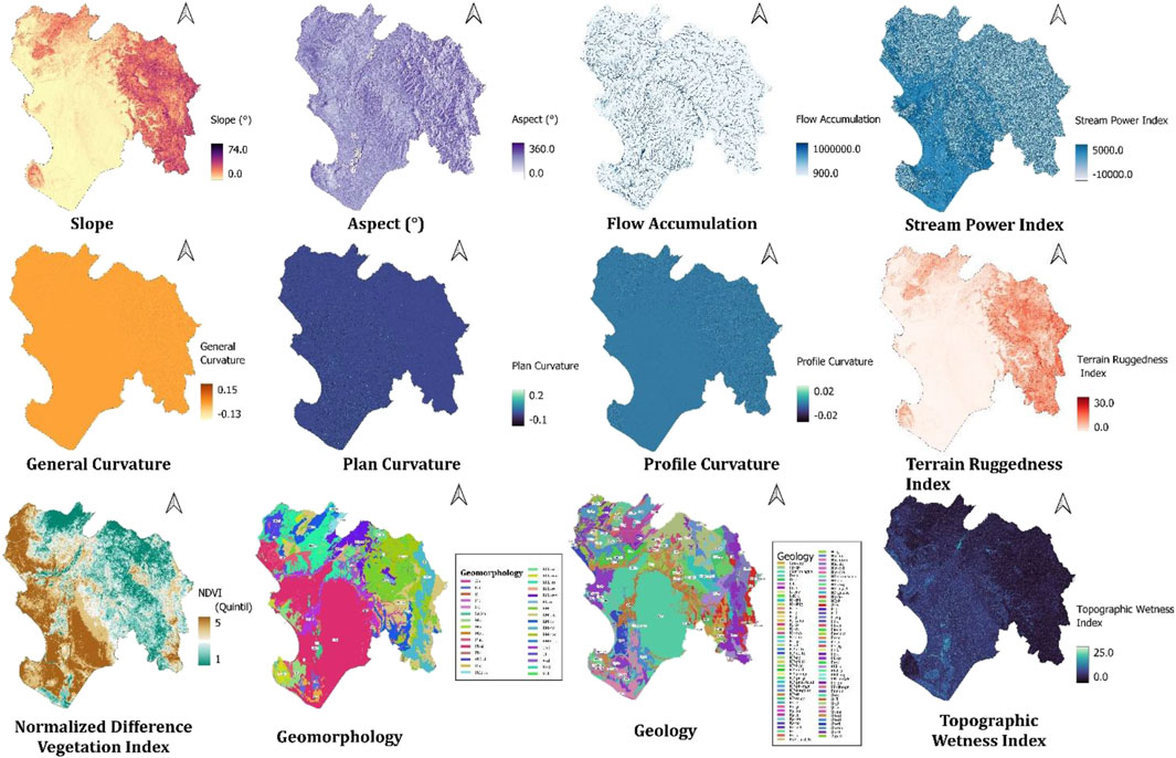
FIGURE A1. Input variables used in the research.

TABLE A1

TABLE A1. Hyperparameters used in this research.