Tropical Dry Forest Resilience to Fire Depends on Fire Frequency and Climate

Hartung, Maximilian; Carreño-Rocabado, Geovana; Peña-Claros, Marielos; van der Sande, Masha T.

doi:10.3389/ffgc.2021.755104

ORIGINAL RESEARCH article

Front. For. Glob. Change, 29 November 2021

Sec. Tropical Forests

Volume 4 - 2021 | https://doi.org/10.3389/ffgc.2021.755104

This article is part of the Research Topic Transformation of Tropical Forests Through Fire View all 6 articles

Tropical Dry Forest Resilience to Fire Depends on Fire Frequency and Climate

$\r\nMaximilian Hartung*$ Maximilian Hartung^1*

Geovana Carreño-Rocabado^2,3

Marielos Peña-Claros¹ $Masha T. van der Sande*\r\n$ Masha T. van der Sande^1*

¹Forest Ecology and Forest Management Group, Wageningen University & Research, Wageningen, Netherlands
²World Agroforestry (ICRAF), Lima, Peru
³Programa Colaborativo de Ecología Aplicada (PCEA), Santa Cruz, Bolivia

Wildfires are becoming increasingly frequent and devastating in many tropical forests. Although seasonally dry tropical forests (SDTF) are among the most fire-threatened ecosystems, their long-term response to frequent wildfires remains largely unknown. This study is among the first to investigate the resilience in response to fire of the Chiquitano SDTF in Bolivia, a large ecoregion that has seen an unprecedented increase in fire intensity and frequency in recent years. We used remote sensing data to assess at a large regional and temporal scale (two decades) how fire frequency and environmental factors determine the resilience of the vegetation to fire disturbance. Resilience was measured as the resistance to fire damage and post-fire recovery. Both parameters were monitored for forested areas that burned once (F1), twice (F2), and three times (F3) between 2000 and 2010 and compared to unburned forests. Resistance and recovery were analyzed using time series of the Normalized Burn Ratio (NBR) index derived from Landsat satellite imagery, and climatic, topographic, and a human development-related variable used to evaluate their influence on resilience. The overall resilience was lowest in forests that burned twice and was higher in forests that burned three times, indicating a possible transition state in fire resilience, probably because forests become increasingly adapted during recurrent fires. Climatic variables, particularly rainfall, were most influential in determining resilience. Our results indicate that the Chiquitano dry forest is relatively resilient to recurring fires, has the capacity to recover and adapt, and that climatic differences are the main determinants of the spatial variation observed in resilience. Nevertheless, further research is needed to understand the effect of the higher frequency and intensity of fires expected in the future due to climate change and land use change, which may pose a greater threat to forest resilience.

Introduction

In recent years, the large and devastating fires burning the highly biodiverse forests of central South America have made international headlines (Bertrand, 2020). Current predictions state that wildfires in the region are expected to become more common due to a complex interplay of climatic and anthropogenic drivers, potentially causing rapid forest dieback (Malhi et al., 2008; Cochrane and Barber, 2009; Andela et al., 2019; Burton et al., 2021). Of the different major South American biomes, dry tropical forests, which are characterized by a distinct dry period, have seen an unprecedented increase in fire occurrence (Di Bella et al., 2006; Pennington et al., 2009), with some areas hit by fires multiple times within the last decades. Here, we assess the resilience to recurring fires of the Chiquitanía in Bolivia, one of the largest remaining dry forests in the Neotropics.

Forest fires have become increasingly common in the Chiquitanía region of Bolivia (Devisscher et al., 2016a), where approximately 17 million ha of forest burned between 2005 and 2019 (Anívarro et al., 2019). This region is home to the Chiquitano seasonally dry tropical forest (SDTF), the largest intact SDTF block in the Neotropics (Pennington et al., 2004). The increasing occurrence of fires in the last decades is particularly alarming due to the lack of understanding of tropical forests’ resilience to fire (Balch et al., 2011) and the fact that dry tropical forests remain largely understudied (Becknell et al., 2012). On the one hand, many ecologists assume that, in contrast to savannas, neotropical SDTFs lack adaptation to fire (Pennington et al., 2009; Power et al., 2016). On the other hand, historical records show that fire has been an integral part of the ecology of the Chiquitanía (Power et al., 2016), and several fire-adapted species with protective traits such as a thick bark are present (Killeen et al., 2006), suggesting that the resilience to fire is higher than generally thought. Much recent work on the effects of fire in the Chiquitanía has been done by Devisscher et al. (2016a, b, 2019), who have found shifts in species composition and functional traits with increasing fire frequency that suggest that the Chiquitanía may irreversibly transition into a more fire-adapted state as fires occur more frequently (Devisscher et al., 2016b). However, their field work mainly focused on transition zones within the Chiquitanía, and it remains unknown whether these changes would be similar across the region. We set out to determine whether these findings scale up over a larger area of the Chiquitanía.

Resilience describes the ability of a system to endure disturbances and consists of two factors, the resistance to a disturbance and the recovery to a pre-disturbance state after the disturbance occurred (Hodgson et al., 2015). The frequency and severity of a disturbance can be crucial in shaping resilience (Ingrisch and Bahn, 2018). Furthermore, several environmental factors can affect the resilience of a forest ecosystem. Water availability and temperature are strong drivers of the distribution of species (Toledo et al., 2012). Additionally, water availability increases tree growth rates and may therefore accelerate the time to reach fire-resistant sizes, leading to increased fire resistance and recovery (Hoffmann et al., 2009; Poorter et al., 2016; Silva et al., 2018). High water availability also reduces fire intensity, leading to less impact on the vegetation and a higher resistance (Schmidt et al., 2017). Increased temperatures, in contrast, exacerbate heat and water stress as well as fire risk, negatively affecting plant development and thus resistance and recovery (Littell et al., 2009; Cook et al., 2014). Both water availability and temperature can further be influenced by topographic features with water availability for example increasing downslope (Markesteijn et al., 2010). Temperature is influenced by topographic features such as the slope orientation, which lead to increased light exposure and can drastically affect surface temperatures over short distances (Lipton, 1992). Finally, human presence and development are known to often negatively influence natural regeneration (Crouzeilles et al., 2020). The majority of wildfires in the Chiquitanía are caused by inappropriate fire practices in the agricultural and livestock sector (Ibarnegaray et al., 2014). Humans thus play a large role in shaping the fire regime and consequently influence the resilience to fire. Hence, the fire regime, environmental factors as well as human presence need to be considered to understand fire resilience.

The fire intensity and frequency observed in the Chiquitanía since the beginning of the millennium are unprecedented, with higher temperatures, dry periods and climate change causing extreme fire intensity and behavior even in non-dry years (Castellnou et al., 2019). Climatic models suggest that temperatures are on the rise whereas rainfall is decreasing in Bolivia, with significant negative consequences for water resources (Seiler et al., 2013). How the Chiquitano dry forest ecosystem will respond to these changes is largely unclear, but this knowledge is urgently required to delineate an action plan moving forward. Doing so is of relevance not only for the scientific interest of better understanding forest resilience but also to preserve areas such as the Chiquitanía on which local communities and biodiversity depend.

Wildfires affect large areas and have long-lasting consequences on the ecosystem. Large-scale approaches spanning several decades are required to measure the fire resilience across an entire region. Remote sensing using satellite imagery that is freely available from online resources offers the opportunity to assess resilience to wildfires over large areas (Di Mauro et al., 2014). Here, we use remote sensing techniques to identify areas burned at different frequencies and to assess their resistance and their recovery during a 10 year period following the last fire. This study is the first to assess the fire resilience of the Chiquitanía at a large regional scale using a remote sensing-derived vegetation index, the normalized burn ratio (NBR). We investigate how results from previous studies at the plot level (e.g., Devisscher et al., 2016b) scale up over the entire Chiquitanía region and identify drivers of spatial variability.

We address two questions. First, what is the effect of fire frequency on the resilience (i.e., the resistance and recovery) of the Chiquitano SDTF? We expect that resilience increases with fire frequency as the abundance of fire-tolerant or fire-adapted species increases. Second, how do environmental factors affect the fire resilience (i.e., the resistance and recovery) of the Chiquitano SDTF? We expect that resilience increases with water availability (through e.g., rainfall and topography) due to weaker fire impacts and faster growth and recovery rates. However, resilience would decrease with temperature due to stronger fire impacts and slower growth rates, and with human presence or pressure, which hampers natural recovery.

Materials and Methods

Study Area

The Chiquitano seasonally dry tropical forest is named after the Chiquitanía, a region in the Eastern lowlands of the Department of Santa Cruz, Bolivia (Figure 1). The Chiquitanía acts as a transition from the humid Amazon forest in the North to the semi-arid Gran Chaco biome in the South (Killeen et al., 2006). Precipitation levels throughout the year range from 500 to 1,710 mm (Killeen et al., 1998). The temperature varies little throughout the year and daily averages are around 24–25°C. The region is marked by its distinct seasonality, with 6 months (beginning in April or May) with <100 mm rain and the driest months being July and August. Annual precipitation levels throughout the Chiquitanía are generally similar, but local differences can be distinguished (Supplementary Appendix 2). The Chiquitanía exhibits a range of deciduousness, with areas receiving less precipitation in the South being fully deciduous and wetter areas in the North tending toward semi-deciduousness (Killeen et al., 2006). Many different vegetation types can be distinguished within the Chiquitanía, several of which have been affected by fire (Anívarro et al., 2019). Generally, forests occur on relatively richer, more fertile soils whereas grasslands are found on sandier, nutrient-poor soils (Devisscher et al., 2016a). We focused on the vegetation type known as Subhumid Semi-deciduous Forest (Bosque subhúmedo semideciduo de la Chiquitanía; henceforth simply referred to as “Chiquitanía”), as defined by Navarro (2011), which covers a substantial part (around 40%) of the Chiquitanía ecoregion (Figure 1, in green, and Supplementary Appendix 1). This vegetation type has been the most affected by fires in recent years (Anívarro et al., 2019). Characteristic species include Acosmium cardenasii, Anadenanthera macrocarpa, Aspidosperma cylindrocarpon, Astronium urundeuva, Caesalpinia pluviosa, Casearia gossypiosperma, Centrolobium microchaete, Guarea macrophylla, Machaerium scleroxylon, Schinopsis brasilensis, Tabebuia impetiginosa (Killeen et al., 2006; Government of Santa Cruz, 2008; Navarro and Ferreira, 2008). The canopy of the dense to semi-dense forest reaches a height of up to 20–25 m and soils are well to moderately well drained (Navarro and Ferreira, 2008; Paz-Roca and Mostacedo, 2020). For the data acquisition, we used the boundaries of the Chiquitanía ecoregion as defined on the web portal GeoBolivia.¹ This area represents the Bosque Modelo Chiquitano, a model forest which encompasses much of Santa Cruz (Anívarro et al., 2019).

FIGURE 1

Figure 1. Location of the study area. Bolivia, in orange, is shown with its departmental subdivision, with the department of Santa Cruz highlighted in yellow. The expanse of the Chiquitanía ecoregion (as defined on GeoBolivia) is shown using a dashed line, with the Subhumid Semi-deciduous Vegetation type (Navarro, 2011), which is the focus of this study, shown in green. The inset (top right) highlights the position of Bolivia on the South American continent.

Google Earth Engine

To assess broad-scale changes in the vegetation after fire, we used remotely sensed data from Google Earth Engine (GEE). GEE is a cloud-based online platform that gives access to high-performance computing resources for analyzing very large geospatial datasets. It offers freely available, analysis-ready remote sensing data (Gorelick et al., 2017). Among many other products, GEE includes satellite data from NASA’s long-running Landsat, Terra and Aqua satellite missions and combines them with a high-performance, parallel computation service. Several studies have already used GEE to perform studies on burned areas and vegetation recovery (e.g., Soulard et al., 2016; Long et al., 2019). All remotely sensed data obtained for this study were retrieved using GEE.

Identifying Burned Areas

The MCD64A1 MODIS Burned Area data product version 6 offered by NASA’s Land Processes Distributed Active Archive Center (LP DAAC) combines data from the Terra and Aqua satellites to obtain monthly, globally burned area at 500 m resolution. MCD64A1 uses MODIS (a sensor aboard Terra and Aqua) surface reflectance imagery in combination with MODIS sensor active fire observations to identify burned areas from the year 2000 onward (Giglio et al., 2015). MCD64A1 was chosen over the MODIS Fire_cci Burned Area pixel product version 5.1 (Chuvieco et al., 2016), also available on GEE, because the latter has been found to be less sensitive to fires in South America (Lizundia-Loiola et al., 2020) and less temporally accurate (Campagnolo et al., 2021). Furthermore, the MCD64A1 product has been validated to perform well by several studies (globally: Padilla et al., 2015; Boschetti et al., 2019; in Brazil: Shimabukuro et al., 2020; Campagnolo et al., 2021; Bolivia: Rodriguez-Montellano et al., 2015) and used in the Chiquitanía for other purposes (Rodriguez-Montellano et al., 2015; Fundación Amigos de la Naturaleza [FAN], 2019).

Using MCD64A1 on GEE, areas were identified that burned at different frequencies within the Chiquitanía between 2000 and 2010. Data from 2010 to 2020 were used to evaluate the forest response following fire. The following four “treatments” were compared:

(1) Control areas that didn’t burn between 2000 and 2020 (Ctrl).

(2) Areas that burned only once between 2000 and 2020, in 2010 (Frequency 1 or F1).

(3) Areas that burned twice between 2000 and 2020, in 2007 and 2010 (Frequency 2 or F2).

(4) Areas that burned three times between 2000 and 2020, in 2002, 2007, 2010 (Frequency 3 or F3).

The years 2002, 2007, and 2010 were chosen because these were years which saw significant fire events (Fundación Amigos de la Naturaleza [FAN], 2019) and have been used in a study in the Chiquitanía previously to evaluate the effect of recurrent wildfire on the vegetation (Devisscher et al., 2016b).

Selection of Sampling Points

For each fire frequency (Ctrl, F1, F2, F3), 500 1-ha plots were randomly selected as sample units (2000 in total). The size of 1 ha was chosen because it is a common standard plot size and because areas need to be larger than 0.5 ha to qualify as forest (FAO, 2020). The selection was performed by creating a grid of adjacent cells 1-ha in size (100 m × 100 m) on top of the study area identified by MCD64A1 using Quantum GIS (QGIS.org, 2021), and 500 random cells were selected using the R 4.0.5 (R Core Team, 2021) for each fire frequency. The spread of the sample units throughout the Chiquitanía decreased with a higher fire frequency (Supplementary Appendix 3).

Normalized Burn Ratio Time Series Analysis

Tracking Vegetation Changes

While the MODIS product MCD64A1 was used to identify burned areas, Landsat 7 satellite data were used to track vegetation changes and measure resilience. The NASA Landsat 7 satellite mission has been collecting spectral information from the Earth’s surface at 30 m spatial resolution approximately every 16 days since April 1999 (U.S. Geological Survey, 2018). Landsat 7 atmospherically corrected surface reflectance imagery was obtained on GEE and Landsat 7 pixels that fell into each sample unit for all available dates between 2000 and 2020 were identified. Clouds, especially prevalent during the rainy season, are a common problem with optical satellite imagery because they do not let through the radiation used for calculating vegetation indices. Furthermore, clouds cast shadows, which can further affect the value of the optical bands within a given pixel. Landsat 7 pixels with more than 25% cloud cover were removed in a first step before using the Quality Assessment bands attached to each pixel to isolate high-quality land pixels that had a low chance of cloud and cloud shadow presence. The Pixel Quality Assessment band is based on the CFMask algorithm (U.S. Geological Survey, 2020). Furthermore, since 2003, Landsat 7 has suffered from the Scan Line Corrector (SLC) failure, which has resulted in gaps in the collected spectral data. SLC-gaps were masked (i.e., made transparent and excluded) for further analyses. Despite these gaps, Landsat 7 still represents one of the most accurate civilian satellite datasets covering large areas of the world (U.S. Geological Survey, 2018).

Vegetation Indices to Assess Resilience

One of the most commonly used remote sensing tools to follow the vegetation state after fire are so-called spectral or vegetation indices (VIs) (Gitas et al., 2012). They are obtained by algebraically combining spectral band values of different wavelengths measured by remote sensors (Gitas et al., 2012). VIs exploit the spectral properties of the environment and vegetation, such as the strong absorption of red light by chlorophyll or reflectance of near-infrared light by the leaf mesophyll (Li et al., 2017). While using information from individual spectral bands offers a simple way of following plant status, this approach may lack sensitivity and makes it difficult to capture the heterogeneity of plant communities on the ground and discriminate between different regions of interest (Xue and Su, 2017). Nonetheless, VIs such as the NDVI (normalized difference vegetation index) or NBR (normalized burn ratio) have been employed in various ways to investigate fire resilience (Díaz-Delgado et al., 2002; Van Leeuwen et al., 2010; Veraverbeke et al., 2012; João et al., 2018; Bright et al., 2019). In our study, the bands in each Landsat pixel were used to obtain a time series of the Normalized Burn Ratio (NBR) vegetation index, spanning the study period (2000–2020), for each pixel. The NBR is similar to the Normalized Difference Vegetation Index (NDVI) but uses the normalized difference between the near-infrared (NIR) and short-wave infrared (SWIR) spectral bands (bands 4 and 7 for Landsat 7):

N B R = \frac{N I R - S W I R}{N I R + S W I R} (Key and Benson, 2006) .

These bands respond strongly, but in opposite ways, to burning, with the NIR band relating to biomass content and the SWIR band relating to the moisture content of the soil and vegetation (U.S. Geological Survey, n.d.). Because each 1-ha sample unit contained several 30 m × 30 m pixels, the NBR values of the Landsat pixels within a given sample unit at a given date were averaged to calculate a single NBR value for that sample unit and date. The region averaging algorithm of GEE considers a Landsat pixel to fall within a defined polygon (such as a sample unit in this study) if 0.5% of that Landsat pixel is included in the polygon (Google Earth Engine, 2021). The NBR was chosen over other indices such as the NDVI due to the NBR’s higher sensitivity to fire damage and to the subsequent structural recovery in both forests and more sparsely vegetated land (Fornacca et al., 2018; Morresi et al., 2019). The NBR is widely used for estimating burn severity and perimeter (Key and Benson, 2006). Vegetation indices relying on short-wave infrared (SWIR) bands are known to better correlate with vegetation and soil moisture, as well as vegetation structure compared to for example the NDVI (Lozano et al., 2007; Hislop et al., 2018), which has known limitations for tracking recovery. These limitations include that the NDVI rapidly increases when forbs, grasses, and other non-woody pioneer vegetation colonize an area soon after disturbance. Furthermore, the NDVI is highly sensitive to leaf-related changes, resulting in its quick saturation following disturbance. The NBR, in contrast, follows recovery in a much more gradual fashion and is thus better fit to track the increase in structural complexity of a forest over time after a disturbance (Pickell et al., 2016). The NBR has been used in several studies to examine post-fire effects on vegetation, including in the Chiquitanía (Dwomoh and Wimberly, 2017; Bright et al., 2019; Maillard et al., 2020).

Sample Unit Quality Check

To check that none of the selected sample units had been converted to agricultural fields or other land types, Sentinel 2 satellite imagery at 10 m spatial resolution was used on GEE to visually confirm which sample units were still “natural” in the first months of 2020 (an example is shown in Supplementary Appendix 4; Sentinel 2 was launched in 2015). All initial 2000 sample units were visually inspected in this manner. Additionally, using the MCD64A1 burned area product, burn dates were obtained for the years 2002, 2007, and 2010 for each sample unit. The majority of fires in 2010 occurred in the months of August and September (Supplementary Appendix 5). Areas that were missing a burn date when they should have burned (e.g., an F3 sample unit missing a burn date in 2002) and areas that had a burn date when they should not have burned (e.g., a control sample unit in any year or F1 in 2002 and 2007) were excluded from the analysis. Furthermore, areas with burn dates outside of the period July 1 up to October 15 (the main fire season) were excluded to ensure that fires happened in more similar seasonal conditions. Out of the original 500 sample units selected for each fire frequency, this resulted in a remaining sample size of 433, 378, 401, and 370 sample units and their associated NBR time series for the Control, F1, F2, and F3 areas, respectively.

Normalized Burn Ratio Time Series Reconstruction

Complete and accurate time series for vegetation index data are crucial for the long-term monitoring of vegetation. Data collected by satellite sensors typically suffer from noise caused by geometric mis-registration, anisotropic reflectance effects, electronic errors, data resampling artifacts, atmospheric effects and clouds. Various methods, such as the interpolation of missing data points and smoothing of time series, are commonly used to reconstruct incomplete or erroneous vegetation index (VI) time series (Cai et al., 2017). In this study, we used both interpolation and smoothing.

Interpolation

To account for missing values within each NBR time series (due to e.g., their removal because of cloud cover), NBR values were linearly interpolated between available time points at intervals of 16 days (equal to the time it takes for the Landsat 7 satellite to fly over the same point over the surface of the Earth) between the first and last available time points in the entire time series. Each sample unit NBR time series was checked to ensure that consecutive time points were indeed always separated by 16 days. Linear interpolation is common for NDVI time series reconstruction (Chen et al., 2004; Fontana et al., 2008; Pan et al., 2015) and has also been applied to time series in dry tropical forests in the Americas (Guzmán et al., 2019). Linear gap filling was done using the na.interpolation function of the R package imputeTS (Moritz and Bartz-Beielstein, 2017) (Supplementary Appendix 6). Sample units with NBR time series that were missing NBR values for more than 12 consecutive time points (equivalent to approximately 6 months, or the length of the dry or wet season) for the year 2001 and for time points between July 2010 and July 2016 (needed for the calculation of resilience metrics later) were excluded from the analysis. This resulted in a remaining final sample size of 157, 146, 213, and 172 sample units and their associated NBR time series for the Control, F1, F2, and F3 areas, respectively.

Smoothing

To minimize any remaining noise and unrealistic values, NBR time series were smoothened using the Savitzky-Golay filter. This filter has consistently been validated in its use to filter out minor fluctuations and create high-quality NDVI time series (Hird and McDermid, 2009; Marcos et al., 2012; Cai et al., 2017; Guzmán et al., 2019). To this end, the sgolayfilt function from the R package signal (Signal developers, 2013) was used. The Savitzky-Golay filter operates as a weighted moving average filter that assigns weights based on a polynomial of a chosen degree (Chen et al., 2004). Two parameters need to be chosen for the Savitzky-Golay filter: p, the order of the polynomial, and m, a parameter which is used to determine the moving average window size, given by 2m+1. In order to best retain the original shape of the NBR time series for each sample unit, different combinations of values for m ranging from 4 to 12 and for p ranging from 1 to 4 were tested and the root mean-squared error (RMSE) between the smoothened and original data calculated. Out of the 36 different parameter combinations, the combination m = 4, p = 4 resulted in the lowest RMSE and was chosen for subsequent analyses (Supplementary Appendix 6).

As a consequence of the interpolation and smoothing process, the data were more balanced and less biased toward the dry season (which has more data due to lower cloud coverage), while still maintaining the overall patterns of the original data (Supplementary Appendices 7, 8).

De-trending the Normalized Burn Ratio Time Series

There are strong seasonal fluctuations in vegetation indices. In order to assess resilience without the confounding effect of seasons, the seasonality signal was removed for each NBR time series through detrending (Figures 2A,B). For each sample unit, NBR time series values were transformed using the Fast Fourier Transform (FFT) to perform frequency domain analysis, also known as Fourier filtering (O’Haver, 1997). The Fourier Transform decomposes a complex function varying over time into a set of simple sine and cosine wave functions, which together add up to the original time series. Each simple function is defined by a given frequency and amplitude. If the frequency of the signal that one wants to remove is known, one can identify this signal among the simple wave functions that make up a more complex function and set its amplitude to 0, effectively filtering it out. Then, an inverse Fourier Transform can be applied to reconstitute the complex function, but this time with the “noise” signal removed. For a seasonal signal repeating every year, one would expect there to be a peak in the frequency domain at a frequency of around 1/365 days or 0.0027 days^–1. This was indeed observed for the NBR time series (Supplementary Appendix 9). In order to remove this signal, signals with a frequency greater than 0.002 (i.e., as frequent or more frequent than every 365 days) were set to 0 and the data transformed back using the Inverse FFT. An example of resulting NBR time series is shown in Supplementary Appendix 9. This procedure is essentially equivalent to using a low-pass frequency filter, common in signal and system analysis. Forward and inverse FFT were implemented using the fft function of the R package stats (R Core Team, 2021).

FIGURE 2

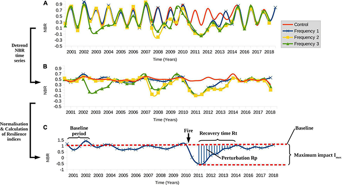
Figure 2. Visualization of the de-trending of the NBR time series and calculation of resilience metrics. (A) NBR time series for illustrative sample units for the different fire frequencies considered in this study. The drops in NBR in the years 2002, 2007, and 2010 represent the fire effects. In each case, the final fire occurs in 2010. (B) The example NBR time series from a. after seasonal de-trending using Fourier filtering. In (A,B), each fire frequency is shown in a different color and line style, defined by the legend at the top right. (C) The seasonally de-trended and base-normalized NBR time series with important values for the quantification of resilience highlighted. For clarity, only the Fire Frequency 1 time series are shown. The following terms are defined: Fire: the date at which fire occurs; Baseline: the pre-fire NBR baseline, derived by averaging NBR values pre-2002; Rp: the post-fire perturbation, indicated by the shaded area between the NBR curve and the baseline between the time point when NBR is lowest and when the baseline is reached again; I_max: the maximum percentage loss in NBR shortly after fire, relative to the baseline. Rt: the amount of time it takes from the lowest NBR value after fire until the baseline is reached again. Together, Rt, I_max and Rp quantify resilience.

Resilience Metrics

To quantify resilience to fire, two measures of resilience, one for resistance and one for recovery, were adopted based on the metrics developed by several authors (Bahn and Ingrisch, 2018; Ingrisch and Bahn, 2018; Carper et al., 2021). Each metric describes a different aspect of the resilience to fire. Taken together, these metrics offer a more complete picture of resilience, as no single metric can fully describe resilience on its own. To allow comparison of these metrics between different sample units, each NBR time series had to be normalized. To this end, a baseline was defined to estimate the pre-fire state of the vegetation. For each sample unit, this pre-fire baseline was calculated by averaging the de-trended NBR values between June 2000 and June 2002, before any fire in the study period occurred. By calculating the baseline from the same years for each sample unit, we avoid differences caused by annual differences in e.g., rainfall. Then, all de-trended NBR values within each time series were baseline-normalized (Ingrisch and Bahn, 2018), i.e., divided by the baseline value, to allow comparison of NBR values. The following metrics were then calculated (Figure 2C).

Resistance

Resistance was determined as the maximum impact, which represents the “maximum deflection of an ecosystem state by a disturbance” (Bahn and Ingrisch, 2018). I_max was calculated relative to the pre-fire baseline as percentage loss (i.e., as negative % values) in baseline-normalized NBR at the lowest NBR value within 6 months of the burn date. I_max thus represents the relative difference between the lowest NBR value after fire and the baseline. For Control areas, the “burn date” was set to August 24 2010, which was the most common burn date. The stronger the impact of fire, the more negative the I_max, and an I_max closer to or above 0 suggests a more resistant system.

Recovery Time

Recovery time was determined as the time to baseline recovery, i.e., the time it takes for a system to return to the pre-disturbance baseline after a disturbance has occurred. By definition, after baseline-normalization, the value of the baseline was set to 1. Recovery time was thus calculated as the time in days it took for a sample unit to reach the pre-fire baseline again after the time point at which I_max was calculated. This metric corresponds to what Holling (1996) termed engineering resilience. A high level of resilience in response to fire should lead to a shorter recovery time to the baseline.

Additionally, we calculated the cumulative fire impact (i.e., the Perturbation Rp), as the cumulative difference between the baseline-normalized NBR curve and the pre-fire baseline from the time point at which I_max was calculated until the baseline was reached again (essentially equivalent to the area between the baseline and the NBR curve). This index represents the overall post-disturbance perturbation, and is the sum of relative differences between the NBR trajectory and the baseline. Rp was calculated by summing the difference between the baseline and the baseline-normalized NBR value for any given date falling within the recovery period Rt. In cases where a disturbance does not cause an overshooting response (i.e., positively affects an ecosystem), Rp is directly related to the mean recovery rate (Bahn and Ingrisch, 2018). As it is independent of the shape of the recovery, it inherently takes into account the variability of recovery rates over time. A more resilient system is expected to have a smaller absolute cumulative difference between the NBR values and the baseline. Because the cumulative impact is strongly correlated with both resistance and recovery time (Spearman correlation coefficients: I_max-Rt: −0.54; I_max-Rp: 0.82; Rt-Rp: −0.88), we here only present results of resistance and recovery and show results of the cumulative impact in Supplementary Appendix. Rt, I_max and Rp were also calculated for the Control areas; this is possible because the NBR time series do not stay perfectly constant over time but fluctuate around the baseline, even for the Controls.

Relation to Fire Severity

The severity of a disturbance can influence resilience (Ingrisch and Bahn, 2018). As Keeley (2009) points out, metrics that combine fire severity and ecosystem responses in a single composite index can be misleading as these metrics may correlate significantly with fire severity measurements in the field but may not actually be very good at predicting ecosystem responses. In our case, it might be difficult to distinguish how much of I_max could be explained by fire severity or the actual ecosystem’s ability to resist the fire. To at least partially address this, we correlated our resilience metrics with the relative differenced normalized burn index (RdNBR), which is a common remote sensing index to measure fire severity (Miller et al., 2009). The RdNBR is given by:

R d N B R = \frac{P r e F i r e N B R - P o s t F i r e N B R}{\sqrt{(| (P r e F i r e N B R / 1000) |)}},

which yields a positive integer that increases in value as the fire severity increases (Miller and Thode, 2007). We used the Savitzky-Golay filtered NBR values obtained from the Landsat image just before a given burn date as PreFireNBR and NBR values from the second Landsat image available after a given burn date as PostFireNBR. The correlation coefficient of RdNBR with I_max, Rt, and Rp was −0.57, 0.13, and −0.40, respectively (the correlation with I_max and Rp is negative because these metrics were defined as negative % losses, i.e., I_max and Rp become more negative as RdNBR or the fire severity increases). As expected, the highest correlation was with I_max, our measure of fire impact, showing that I_max captures the effects of fire impact to some extent. These correlations are given for reference here, but this study focuses on the resilience metrics that we describe above. All metrics were computed in the R programming environment version 4.1.0 (R Core Team, 2021).

Environmental Predictors

We identified a total of 14 variables related to climatic, human-related and topographic factors that can potentially influence I_max, Rp, and Rt. These variables may influence the presence and intensity of fires and the recovery of vegetation, and were subsequently obtained for each of the sample units using GEE. The following subsections cover the different variables in more detail.

Climatic Data

Climatic data were obtained for each sample unit for the study period (2000–2020) using the TerraClimate product, available on GEE. TerraClimate represents a high-resolution (2.5 arc minutes) dataset that offers monthly climate and water balance data from the years 1958–2019. It uses climatically aided interpolation and combines high-spatial resolution climatological normals from the WorldClim dataset with time series from the CRU Ts4.0 and Japanese 55-year Reanalysis dataset (Abatzoglou et al., 2018). Among other variables, the TerraClimate dataset offers monthly precipitation, monthly minimum temperature and monthly maximum temperature data. To determine whether the TerraClimate dataset adequately described climatic variables in the Chiquitanía, TerraClimate precipitation, maximum temperature, and minimum temperature data at the coordinates of seven weather stations in the Chiquitanía were compared to ground measurements from those same weather stations obtained from the Bolivian national service of meteorology and hydrology (SENAMHI, data available on http://senamhi.gob.bo/). Using the mean absolute error (MAE) as a metric for comparison, the mean MAE for monthly precipitation was around 42 mm while it was less than 1°C for either minimum and maximum temperature (Supplementary Appendix 10). The TerraClimate data were used in the remainder of this study given their accuracy and the possibility to obtain data at the level of the sample units used in this study. Using R, these variables were used to calculate the mean annual precipitation, mean annual minimum temperature, mean annual maximum temperature and mean annual rainfall seasonality (the coefficient of variation of monthly precipitation values) for each sample unit between 2000 and 2020.

Human Influence

Areas linked to human use and close to human-impacted areas (e.g., forest edges) can be most strongly impacted by forest fires (Maillard et al., 2020). To incorporate the aspect of human influence into the study, the global human modification (gHM) dataset published by Kennedy et al. (2019) was obtained. This dataset provides an index that estimates the cumulative intensity of human modification associated with several different types of human-associated “stressors,” such as human settlement, agriculture and infrastructure for the year 2016 for pixels at 1 km resolution. The gHM index ranges in value from 0 as the lowest level of human modification up to 1 representing the highest level of human modification or stress. The gHM values for each sample unit were extracted using GEE (Supplementary Appendix 11).

Topographic Data

Topographic features can strongly influence the resilience of trees to fires by affecting vegetative spatial patterns across the landscape (Ng et al., 2020). Elevation and slope can favor regeneration because higher and steeper areas are often associated with lower accessibility for humans and a wetter climate, which is often associated with a positive effect on recovery (Thomlinson et al., 1996; Crk et al., 2009). Furthermore, aspect can be important, as moisture-bearing trade winds are often directional, releasing more moisture on slopes facing a certain direction (Crk et al., 2009), and a given slope orientation can lead to increased light exposure and drastically affect surface temperatures over short distances (Lipton, 1992). Generally, insolation and topographic position can influence the risk of fire as they affect both surface temperature and water availability (Kane et al., 2015a, b). Water availability tends to increase downslope and crest positions are usually significantly drier than valleys and slopes (Markesteijn et al., 2010). Topographic position can be described by the topographic position index (TPI), which relates the position of a given point to its surroundings. It is calculated by taking the difference between the elevation of a given point X and the mean elevation of points within a continuous ring of a given radius (an annulus) centered on X. Positive values indicate that X is located higher than its specified neighborhood (Weiss, 2001).

Elevation was extracted from GEE using the NASA SRTM Digital Elevation 30m dataset (Farr et al., 2007). Aspect and slope were derived from the elevation dataset using built-in functions of GEE. Insolation was estimated by using the solar radiation index (SRI) given by:

S R I = 1 + c o s (l a t i t u d e) \times c o s (s l o p e) + s i n (l a t i t u d e) \times s i n (s l o p e) \times c o s (a s p e c t) (Kane et al., 2015b)

which ranges from 0 to 2, with 0 being the lowest level of solar radiation and 2 the highest. The SRI models the level of solar radiation around noon on the equinox (Keating et al., 2007). The TPI, being scale-dependent, was calculated for annuli of radii 100, 250, 500, 1,000, and 2,000 m, following Kane et al. (2015b).

Data Analysis

Effect of Fire Frequency

To assess the differences between the different fire frequencies in the resistance and recovery, we ran Kruskal-Wallis tests with resistance (I_max) or recovery time (Rt) as response variable and fire frequency as explanatory factor. A Dunn test was subsequently used with the Bonferroni correction to perform multiple comparisons. Additionally, we tested for differences in the baseline and the perturbation (Rp) between the fire frequencies. All statistical analyses were implemented in R using the stats package for the Kruskal-Wallis test (R Core Team, 2021) and the FSA (Ogle et al., 2021) and rcompanion (Mangiafico, 2021) packages for multiple comparisons. The exact results for the multiple comparisons are given in Supplementary Appendix 12.

Effect of Environmental Factors

To assess the influence of environmental variables on the resilience indices I_max, Rt, and Rp, multiple linear regressions and random forest models were developed with the resilience indices as response variables. To avoid multicollinearity, the Spearman correlation test was run between all the predictor variables using the Hmisc R package (Harrell and Dupont, 2021). A correlation coefficient threshold of 0.70 was used to remove correlated predictors. Only the variable that more strongly correlated with the response variables I_max, Rp, and Rt was kept (Supplementary Appendix 13). Consequently, elevation, maximum temperature and TPI at 100, 250, 500, and 2,000 m were removed from the dataset. Because differences in the pre-fire baseline between the different fire frequencies were observed in the Kruskal-Wallis tests, the baseline and the fire frequency were also included in the models as predictor variables. Thus, the predictor variables used were Fire Frequency, Pre-Fire Baseline, Mean Annual Precipitation, Mean Annual Rainfall Seasonality, Mean Annual Minimum Temperature, gHM, slope, aspect, SRI, and TPI at 1,000 m. Because the goal of this analysis was to investigate the effect of the predictor variables on the resilience of areas that had been affected by fire, Control areas were excluded from the analysis. A table giving descriptive statistics of the different variables considered with and without the Control areas is given in Supplementary Appendix 14.

Linear Regression

Linear regression models were used to determine (1) which variables had an influence on the resilience indices, (2) what the direction of the relationship was and (3) whether the effect of variables differed between different fire frequencies. In order to satisfy the requirements of linear regression, Rp values were cubic root transformed. Because the recovery time Rt is a count variable, a generalized linear model with a Poisson distribution was initially tried for Rt. However, the variance was larger than the mean, thus a generalized linear model using the negative binomial distribution was eventually fitted. Fitted values vs. observed values from both models were compared to assess if a negative binomial distribution was better for our data. A backward selection method was used to identify a more parsimonious set of predictor variables and any significant interactions between frequency and the other predictor variables were added. Numerical predictor variables for the parsimonious model were scaled by subtracting the mean and dividing by the standard deviation to facilitate model output interpretation. Linear models were built using the lm function from the stats package in R (R Core Team, 2021), whereas the glm.nb function from the MASS package in R was used for building generalized linear models (Venables and Ripley, 2002).

Random Forests

The random forest supervised learning algorithm (Breiman, 2001) was used to determine (1) how well the different environmental variables, the pre-fire baseline and the fire frequency predicted the variation in Rt, I_max, and Rp, and (2) which predictor variables had the highest influence in these predictions. A random forest is a collection of multiple randomly developed decision trees, which are combined to produce a final model. Because the trees are developed randomly, a random portion of the data fed into the algorithm are used to train the model while the remainder (out-of-bag data) is used for model validation. This results in a metric known as variance explained, which is similar to the R² in linear regressions. The algorithm also provides a measure of predictor importance, which is computed by using randomly permutated out-of-bag data for a single predictor in all the random forest trees. The change in mean square error compared to the original out-of-bag data then represents the variable importance (Kane et al., 2015b). While importance scores are often normalized to more easily compare importance scores across models, it has been suggested that raw importance scores have better statistical properties (Strobl et al., 2008).

For each random forest model predicting either Rt, I_max, or Rp, 75% of the data were used for training the random forest while the rest were used for validation. We report both the explained variance based on out-of-bag data and the R² obtained by calculating how well each random forest predicts the set-aside validation data. We finally report the raw importance scores for each predictor variable in each random forest. The number of trees used in each model was set to 1,000 to obtain stable results while the number of variables to be used in each split (mtry) was optimized by testing mtry values between 1 and 10 and picking the mtry value that resulted in the lowest mean squared error in the final model. This resulted in mtry values of 4, 3, and 5 when Rt, I_max, Rp were the dependent variable, respectively. Random forests were built using the randomForest package (Liaw and Wiener, 2002).

Results

We set out to determine the resistance and recovery of the Chiquitanía using the NBR remote sensing index following fires in 2010 for areas did not burn (Ctrl), that burned once (F1), twice (F2), or three times (F3), and what factors might influence this resilience.

Effect of Fire Frequency

A significant effect of fire frequency (0, 1, 2, or 3 fire events) on the resistance I_max and the recovery time Rt was found (Figure 3). The resistance (I_max) was similar between areas that experienced fire, but tended to decrease from F1 to F2 and increase from F2 to F3 (Figure 3A). The recovery time Rt was longer for F1 (median: 576 days) and F2 (median: 592 days) than it was for F3 (median: 240 days), which did not differ significantly from the Control (median: 208 days; Figure 3B). Note that 2010 was also a drought year, likely leading to non-zero resistance and recovery also of control areas. All areas showed full recovery to the pre-fire baseline within the time frame considered. The perturbation Rp showed similar results to I_max (Supplementary Appendix 15). Moreover, the pre-fire baseline was lower for F3 and highest for control areas (Supplementary Appendix 15).

FIGURE 3

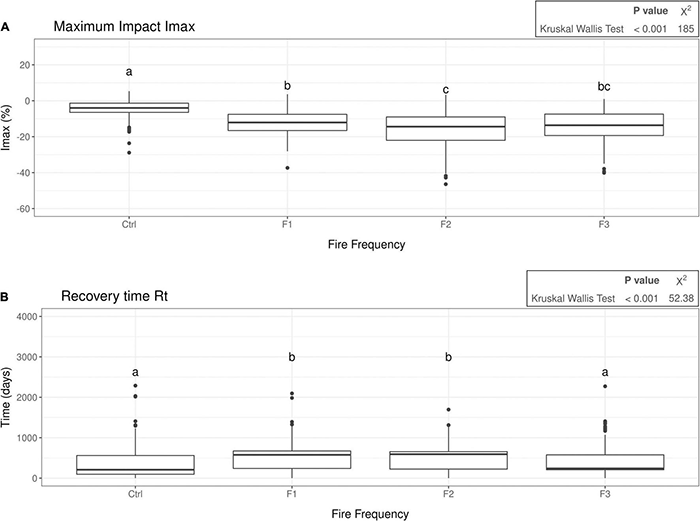
Figure 3. Box plots showing the maximum fire impact (I_max) (A) and the recovery time to the baseline (Rt), i.e., the number of days after fire (or Aug 24 2010 for Control data points) until the baseline is reached again (B) and how they differ between the fire frequencies (Ctrl = control, no fire; F1 = 1 fire event, F2 = 2 fire events, F3 = 3 fire events). Both Rt and I_max were calculated for the fire in the year 2010 and are measures of the recovery and resistance, respectively. The letters at the top of each box plot represent the significance groups obtained after a multiple comparison test. The output of the Kruskal-Wallis test (p-value and Chi squared statistic) is shown at the top right of each box plot.

Effect of Environmental Factors

Linear Regression

A multiple linear regression and generalized linear model with negative binomial distribution were, respectively, used to predict I_max or Rt based on several predictor variables. The most parsimonious model for I_max, the measure of resistance, showed that the pre-fire baseline and slope increased I_max (i.e., the impact was lower), TPI 1000 and minimum temperature decreased I_max while precipitation decreased I_max for F1 and F2 but increased I_max for F3 (Figure 4A). The adjusted R² of the model was 0.28 (residual standard error = 7.55 on 521 degrees of freedom and F-statistic = 23.77). Similar results were seen for the cumulative impact Rp (Supplementary Appendix 16). The most parsimonious model for Rt, the measure of recovery, showed that slope and minimum temperature shortened the recovery time, rainfall seasonality increased the recovery time, while precipitation increased the recovery time, especially for F2 (Figure 4B). The global human modification index was not significant in any model and thus not included in the final models. The full model details are given in Supplementary Appendix 16. The differences between the different fire frequencies in the linear regression models were similar to the ones observed in Figure 3, which is why we do not show these differences in Figure 4 and omit the intercept values for clarity (see Supplementary Appendix 16).

FIGURE 4

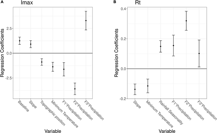
Figure 4. Regression coefficients for several variables predicting the maximum impact I_max (A) or the recovery time Rt (B). A multiple linear regression and generalized linear model with negative binomial distribution were used to predict I_max or Rt, respectively. Error bars show standard errors and interactions are indicated by an asterisk. Estimates for the regression model intercepts are not shown.

Random Forest

R² values of the random forest models predicting Rt, I_max, and Rp calculated for out-of-bag data ranged from 23 to 40%, while the R² obtained for data that were not used in training the models ranged from 30 to 47% (Figure 5 and Supplementary Appendix 17). In every model, precipitation was assigned the highest importance score, followed by rainfall seasonality and minimum temperature (Figure 5). Topographic variables exhibited smaller importance scores, with slope being the most important topographic variable. Fire frequency had an importance score similar to the topographic variables in all models. The solar radiation index (SRI) and aspect consistently scored lowest in importance and were close to 0. Human modification, estimated by the global human modification (gHM) variable, generally scored low. The pre-fire baseline was important for Rt and I_max, but less so for Rp (Supplementary Appendix 17).

FIGURE 5

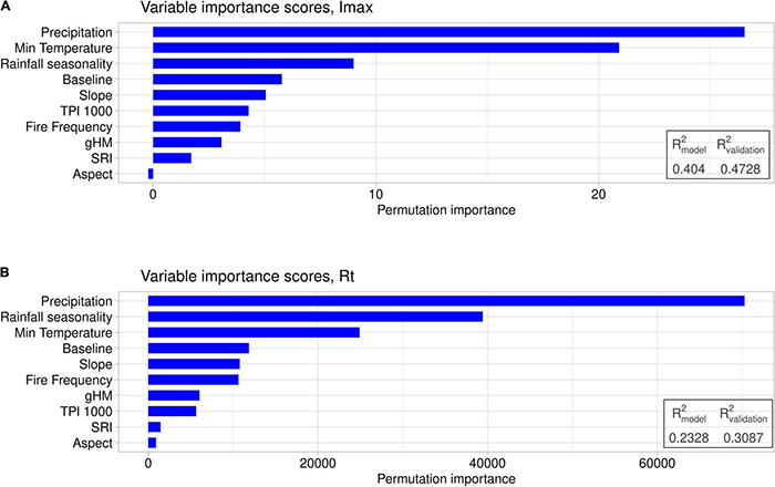
Figure 5. Variable importance scores for the random forests with the maximum impact (Imax; A) or the recovery time to the baseline (Rt; B) as dependent variable. The predictor variables are indicated on the y-axis and are the same for each model. Importance scores are given as the permutation importance, which is the increase in mean squared error of the model when the values of a given predictor variable are randomly shuffled and the model run again. The importance scores are given in absolute terms rather than being normalized, and allow comparison between the relative predictive strengths of each variable.

Discussion

Fire Resilience of the Chiquitano Dry Forest

We used the remote sensing index normalized burn ratio (NBR) to analyze the resilience of the Chiquitano dry tropical forest. Our results are summarized in Figure 6, which offers as spatial representation of the distribution of resistance and recovery values across the Chiquitanía (the spatial map for Rp is given in Supplementary Appendix 18). We expected that areas that burned at different frequencies would have lower resilience than control areas that did not burn. Indeed, control areas had a maximum impact (I_max) and recovery time (Rt) that were closest to 0 and significantly different from areas that experienced fire (Figure 3), indicating a significant effect of fire in 2010 on the vegetation in burned areas. Deviations from 0 for the control may be caused by the major drought in 2010 (Devisscher et al., 2016a), which likely caused tree mortality and therefore changes in the vegetation indices. The average impact of the 2010 fire was low to moderate (Figure 3A, median drop relative to the baseline lower than 20% for all fire frequencies). Moreover, the majority of areas affected by fire recovered to baseline levels very fast, within 2–3 years (Figure 3B). The relatively high fertility of soils and general edaphic variability in the Chiquitanía, together with the presence of fire-tolerant species (Iporre, 1996; Killeen et al., 2006; Toledo et al., 2012) may facilitate relatively fast vegetation recovery following fire. It has been observed that different vegetation types of the Chiquitanía, including the subhumid semi-deciduous forest, display high resilience to fire in the Chiquitanía (B. Mostacedo, personal communication, July 22, 2021). Much of the vegetation regenerates within 6 months following the fire, with few traces of fire left; trees show a high survival rate (around 70%), with new trees being primarily recruited through seed dispersal, and to a minor extent through re-sprouting (B. Mostacedo, personal communication, July 22, 2021). Reproductive strategies can play an important role in the ability to recover after fire, which is why tree species composition and the presence of nearby seed sources are crucial in determining the future of forests facing extreme weather and fire conditions (Brando et al., 2014). 62% of canopy species in the Lomerío region of the Chiquitanía have been found to be wind-dispersed (Justiniano and Fredericksen, 2000) and several tree species in a dry forest in Brazil (many of which are also found in the Chiquitanía) have shown a strong ability to re-sprout (Vieira et al., 2006). These traits allow dry forest species to better colonize disturbed areas (Vieira and Scariot, 2006), and to become more abundant as fire becomes more frequent. Tree regeneration in the Chiquitanía may, however, be hampered by the proliferation of herbaceous vines and lianas after fire (Pinard et al., 1999). Indeed, lianas can re-sprout from roots that are able to survive fire events (Mostacedo et al., 2001). Nevertheless, fire has been a persistent feature of the natural history of the Chiquitanía (Power et al., 2016), which suggests that the forest is highly resilient and capable of sustaining itself following fire. It remains unclear, however, if there exists a threshold in fire intensity or frequency which, if exceeded, may lead to substantial forest dieback (Balch et al., 2011). Intensifying fire regimes in the future may lead to a decrease, instead of an increase, of the fire resilience.

FIGURE 6

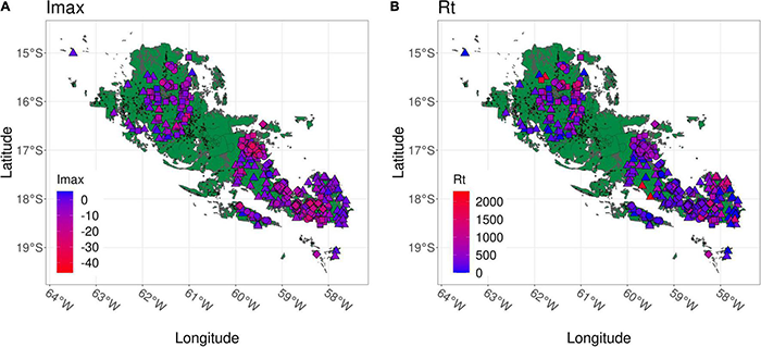
Figure 6. Spatial map showing the distribution of plots and values of the resilience metrics. (A) Maximum impact I_max (expressed as percentage loss) and (B) recovery time Rt, the number of days after fire (or Aug 24 2010 for Control data points) until the baseline was reached again. Each shape corresponds to a plot experiencing a different fire frequency ( www.frontiersin.org : Ctrl = control, no fire; ▲: F1 = 1 fire event; ■: F2 = 2 fire events; ◆: F3 = 3 fire events), whereas the color gradient of each point indicates the higher or lower values of the resilience metric. The area corresponds to the area in green in Figure 1.

Fire Resilience Is Lowest at Intermediate Fire Frequency

We expected that resilience would increase with fire frequency, i.e., that resistance would increase and recovery time would decrease as fire frequency increased for burned areas. Overall resilience was lower for F2, with lower I_max and higher Rt values indicating lower resilience, while F1 and F3 appeared more resilient (Figure 3). Devisscher et al. (2016b) observed similar results; they found that biomass reduction after fire in the Chiquitanía was higher (i.e., resistance was lower) after two fires compared to areas that had burned once or three times. Several interacting effects possibly explained the higher biomass reduction for F2, such as the presence of trees that died during or following the first fire as a consequence of damage suffered in the first fire, but only burned in the second fire; pioneer species colonizing the area after the first fire which may have been more vulnerable to fire; too little time for young trees to reach fire-resistant sizes after the first fire (Devisscher et al., 2016b). By the time the third fire occurred, the fuel left to burn had likely been reduced, leading to less severe fires. Moreover, the species present (e.g., Anadenanthera, Astronium, Tabebuia) were likely mostly fire-tolerant with thick bark to protect from fire damage (Devisscher et al., 2016b). However, it remains unclear whether these changes would constitute a resilient response, i.e., of an ecosystem returning to its pre-fire state, or an adaptive response, i.e., an ecosystem that changes in the final suite of species present compared to the pre-fire state. Important shifts in species composition with increased fire occurrence have been observed in several biomes (e.g., the Brazilian Amazon—Barlow and Peres, 2008; Tasmania—Harris et al., 2018), suggesting that many forest ecosystems undergo adaptive responses to fire in the short term. It is further possible that some of the results presented here may be biased due to different pre-fire baseline levels for the different plots (further discussed below).

Climate Drives Fire Resilience

We expected resilience to vary across the region and increase with increasing water availability (e.g., high precipitation and low seasonality) and to decrease with increasing temperature. We indeed found that climatic variables were most influential in predicting resilience (estimated by I_max and Rt), with precipitation representing the most important climatic variable (Figure 5). The precipitation effect on resistance, however, differed between the fire frequencies; whereas precipitation indeed had a positive effect on resistance in areas that burned three times, it had a negative effect on the resistance of areas that burned once or twice. Precipitation decreased recovery (i.e., increased recovery time) across all fire frequencies. The contrasting effect of precipitation for F1 and F2 vs. F3 observed for I_max may be the result of a shift in vegetation community structure. Water availability plays a key role in the distribution of species in lowland tropical forests and the presence of species along a water availability gradient is influenced by their drought tolerance (Markesteijn and Poorter, 2009). In regions with high precipitation, the baseline community will consist of a higher proportion of species that prefer somewhat wetter climates and are comparatively less drought- and fire-tolerant. Therefore, in the absence of multiple previous fires, the wetter areas harbor less fire-tolerant communities that result in lower fire resilience. However, as mentioned before, recurring fires can cause fire-tolerant species to become more dominant (Devisscher et al., 2016b). In areas with recurring fire, the rainfall gradient may no longer represent a fire-tolerance gradient. Instead, the resistance of such relatively fire-tolerant communities may increase with rainfall because of less severe fires and enhanced growth rates that can lead to e.g., thicker bark. Hence, in areas with low fire frequency, the rainfall gradient represents the original species composition and its tolerance to fire, whereas at higher fire frequency, the vegetation composition may have shifted toward more fire tolerant species and higher water availability results in less fire damage. At the same time, rainfall decreased recovery for all fire frequencies. Gazol et al. (2017) observed that forests in drier regions in Europe and North America had a greater recovery capacity following drought, indicating a greater ability to adapt and respond to periods of disturbance. Trees growing in drier environments tend to invest more in below-ground biomass (Markesteijn and Poorter, 2009), thus improving their ability to access water. Moreover, trees experiencing water stress can be relatively more efficient in their use of water (Tong et al., 2019) and may show an increased storage of carbohydrates (Granda and Camarero, 2017), which may allow them to recover faster after disturbance by fire compared to trees growing in wetter conditions. Thus, the negative effect of rainfall may point to a more general trade-off that plants are subject to regarding their resource allocation, and consequently also resistance and recovery.

Rainfall seasonality (the coefficient of variation of rainfall) decreased recovery (i.e., increased recovery time). The negative effect of rainfall seasonality on recovery could indicate that the dry season is more pronounced, i.e., that the growing season is shorter, as the seasonality increases, which can hamper recovery. Rainfall variability exerts great control over biological processes and can cause scarcity and mortality in dry months (Schwartz et al., 2020). Interestingly, recovery, but not resistance, was affected by rainfall seasonality. Resistance can manifest itself through traits such as a thick bark (Mostacedo et al., 2001), which confers more resistance as the bark grows over the course of a plant’s life. Hence, resistance is age-dependent. Conversely, recovery may rely more on conditions present at the time of recovery, potentially explaining why the rainfall seasonality would affect recovery, but not resistance.

Average minimum temperature decreased resistance but increased recovery (i.e., shortened the recovery time). The negative effect of minimum temperature on resistance may be caused by increased evaporation at high temperature, which increases and exacerbates dry events (Littell et al., 2009; Cook et al., 2014) and may therefore lead to more intense and devastating fires (Littell et al., 2016). Indeed, constantly higher temperatures were at the root of the devastating fires in the Chiquitanía in 2019 (Castellnou et al., 2019). Conversely, minimum temperature had a positive effect on recovery by shortening the recovery time, possibly because higher minimum temperature, up to a certain point, can accelerate plant growth rates and thus recovery.

Rainfall and temperature have been shown to be strong drivers of species distribution in Bolivia (Toledo et al., 2012). At the same time, recurring fires may lead to increased dominance of fire-tolerant species (Devisscher et al., 2016b). Our results support these studies and suggest that both the climate and fire frequency determine fire resilience.

Resilience Increases on Steep Slopes and in Valleys, but Is Not Affected by Human Influence

We expected factors increasing the level of insolation (such as aspect or the solar radiation index SRI) to decrease fire resistance by creating drier conditions but to increase recovery due to increased growth. Variables influencing insolation scored consistently lowest in importance in predicting resilience, whereas topographic position and particularly slope played a more significant role (Figure 5). Slope increased both resistance and recovery (by reducing recovery time), while higher topographic positions decreased resistance and recovery (Figure 4). Steeper terrain is often associated with lower accessibility to humans and thus less development, which can have a positive effect on forest recovery (Crk et al., 2009). While steeper slopes may be associated with more severe fire effects (Lentile et al., 2006), because unburned fuel ahead of the fire is preheated as the fire climbs upslope (DeBano et al., 1998), water availability may be relatively higher on slopes and in valleys than on hilltops, leading to less severe fires and higher fire resistance and recovery (Markesteijn et al., 2010; Lee et al., 2018). However, the effects of topography can be complex, and their lower importance scores in the random forests may point to the fact that other factors (such as climate) play a more dominant role in shaping resilience.

Although the vast majority of fires in the Chiquitanía can be linked to human activities such as slash-and-burn agriculture (locally referred to as chaqueo) (Devisscher et al., 2019), we found no effect of human influence (measured by the human modification index) on fire resilience. Generally, the degree of human modification was low for the areas considered in this study (Supplementary Appendix 14) and rather homogeneous throughout the whole region. It is possible that people choose to burn forests also in more remote areas where the levels of human modification are low and where large tracts of forests can be converted for agricultural purposes. Therefore, the proximity to human settlements or infrastructure (e.g., roads) may be more important to describe the effect of presence of humans on fire resilience in the Chiquitanía. It may also be that another index than the one chosen in this study is more appropriate for an area with a relatively low human population density such as the Chiquitanía. Alternatively, it may be that indices measuring human influence may explain where fires occur, but not their intensity or the resistance and recovery of the ecosystem, which are more determined by the climate and the vegetation composition.

Pre-fire Baseline Effects

We cannot know whether fire occurred before the start of the study period (i.e., before 2000). Given that the pre-fire baseline values decrease at higher fire frequency (Supplementary Appendix 15), it is likely that some areas are more prone to receive fires, leading to a lower baseline. A lower initial baseline, such as in the case of areas that burned three times, may lead to a faster recovery to baseline levels. Future research will need to investigate what factors can explain the likelihood of areas to be affected by fire. The pre-fire baseline had a positive effect on resistance (Figure 4), suggesting that forests with higher initial vegetation values suffered less severe fire impact. Baselines are often dynamic, and it is common to use a pre-disturbance state to estimate a baseline (Bahn and Ingrisch, 2018). For the Chiquitanía, it is unrealistic to expect to find areas without any fire history, as fires have been present throughout the Holocene (Power et al., 2016). Rather than thinking of the areas considered here as areas that burned exactly one, two, or three times, it is perhaps more useful to think of these areas as falling on a spectrum of areas in which fires have occurred more or less frequently.

The Future of the Chiquitano Dry Tropical Forest

The Chiquitanía represents an important source of timber, water, game, construction material, and non-timber forest products (Devisscher et al., 2019). Fire also causes large-scale disturbances of the soil structure, soil nutrients, and local hydrology (Wells, 1979; Maass et al., 1988; Stoof, 2011). Ten out of sixteen important drainage basins in Santa Cruz are located in the Chiquitanía, all of which have already been affected by fire, with potential risks for both the humans and the local ecosystem (Anívarro et al., 2019). The majority of fires in the Chiquitanía can be traced back to human activity, often in conjunction with inappropriate fire practices in the agricultural and livestock sector (Ibarnegaray et al., 2014). Engaging with stakeholders is thus key to address the urgent issue of fires in the Chiquitanía.

Conclusion

We show that the Chiquitanía dry forest is relatively resilient to up to three recurrent fires. This resilience initially decreases, but then increases again after the third fire, which may point toward an ecological transition state toward a higher abundance of fire-tolerant species with recurring fires. Climatic factors, especially water availability, are more important in shaping resilience than topography and human influence. As droughts and fires are becoming more common due to the growing threat of climate change and land use change, the Chiquitanía region is facing considerable challenges in the future. Long-term monitoring, combining remote and ground-based data building on the results of this study, will be important for understanding the long-term resilience of the Chiquitano ecosystem and for protecting the lives and livelihoods that depend on it. Such knowledge will be the basis of adequate management and restoration efforts of one of the largest remaining tropical dry forests. Hence, although the current ecosystem seems to possess still high fire resilience, its future with more frequent and intense fires and droughts remains uncertain.

Data Availability Statement

The datasets presented in this study can be found in online repositories. The names of the repository/repositories and accession number(s) can be found below: upon acceptance and publication of the manuscript, all data underlying the analyses will be published in the open access data repository DANS (https://dans.knaw.nl).

Author Contributions

MH collected, processed, analyzed the data, and wrote the first draft. All authors discussed the results, contributed to the revisions, conceived the idea, and designed the study.

Funding

MS was supported by the Veni Research programme with project number NWO-VI. Veni.192.027 and the project NWO-ALW.OP24.

Conflict of Interest

The authors declare that the research was conducted in the absence of any commercial or financial relationships that could be construed as a potential conflict of interest.

Publisher’s Note

All claims expressed in this article are solely those of the authors and do not necessarily represent those of their affiliated organizations, or those of the publisher, the editors and the reviewers. Any product that may be evaluated in this article, or claim that may be made by its manufacturer, is not guaranteed or endorsed by the publisher.

Supplementary Material

The Supplementary Material for this article can be found online at: https://www.frontiersin.org/articles/10.3389/ffgc.2021.755104/full#supplementary-material

Footnote

^ http://geo.gob.bo/portal/

References

Abatzoglou, J. T., Dobrowski, S. Z., Parks, S. A., and Hegewisch, K. C. (2018). TerraClimate, a high-resolution global dataset of monthly climate and climatic water balance from 1958–2015. Sci. Data 5:170191. doi: 10.1038/sdata.2017.191

PubMed Abstract | CrossRef Full Text | Google Scholar

Andela, N., Morton, D. C., Giglio, L., Paugam, R., Chen, Y., Hantson, S., et al. (2019). The Global Fire Atlas of individual fire size, duration, speed and direction. Earth Syst. Sci. Data 11, 529–552. doi: 10.5194/essd-11-529-2019

CrossRef Full Text | Google Scholar

Anívarro, R., Azurduy, H., Maillard, O., and Markos, A. (2019). Diagnóstico por Teledetección de Áreas Quemadas en la Chiquitanía. Informe técnico del Observatorio Bosque Seco Chiquitano. Santa Cruz de la Sierra: Fundación para la Conservación del Bosque Chiquitano.