Abstract
Published biogenic volatile organic compound (BVOC) emission rates of Norway spruces vary a lot. In this study we combined published Norway spruce emission rates measured in boreal forests and added our new, unpublished emission data from Southern (SF) and Northern Finland (NF). Standardized summer monthly mean emission potentials of isoprene vary from below the detection limit to 7 μg g–1(dw) h–1, and monoterpene (MT) and sesquiterpene (SQT) emission potentials 0.01–3 μg g–1(dw) h–1 and 0.03–2.7 μg g–1(dw) h–1, respectively. In this study, we found much higher SQT emissions from Norway spruces than previously measured, and on average SQTs had higher emission potentials than isoprene or MTs. The highest monthly mean SQT emission potential of 13.6 μg g–1(dw) h–1 was observed in September in Southern Finland. We found that none of the younger (33–40 years) trees in Hyytiälä, Southern Finland, emitted isoprene, while one 50-year-old tree was a strong isoprene emitter. The difference due to age could not be confirmed, since all measured small trees were growing in Hyytiälä, so this could also be due to the same genetic origin. On average, older trees (>80 years) emitted about ten times more isoprene and MTs than younger ones (<80 years), but no clear difference was seen in SQT emissions. SQT emissions can be more related to stress effects. As shown here for Norway spruce, it is possible that the emission factor of SQTs is significantly higher than what is currently used in models, which may have significant effects on the prediction of formation and growth of new particles, since the secondary organic aerosol (SOA) formation potential of SQTs is high, and this may have significant effects on the formation and growth of new particles. Due to the high secondary organic aerosol (SOA) formation potentials of SQTs, the impact on SOA formation and mass could be even higher.
1. Introduction
Boreal forest covers about 11⋅106 km2., i.e., about 30% of the world’s forests (Pan et al., 2013). The amount of tree species is not very diverse, consisting mainly of conifers such as pines and spruces, and larch species (Soja et al., 2007). Some broadleaved deciduous trees are also common and include, e.g., Betula sp., Alnus sp., and Populus sp. Terrestrial vegetation, mainly trees, emit large amounts of volatile organic compounds (VOCs) to the atmosphere, impacting the formation of ozone, secondary organic aerosol (SOA), and clouds (e.g., Yli-Juuti et al., 2021). Even small changes in VOC emissions in boreal areas for example due to changing climate, may substantially modify the radiative properties of clouds (Petäjä et al., 2022). Biogenic VOC (BVOC) emissions dominate global VOC emissions consisting mainly of isoprene (ISOP), monoterpenes (MT), sesquiterpenes (SQT), methanol and acetone (Sindelarova et al., 2014). While isoprene and terpenes are known to have strong impacts on aerosol formation, the role of methanol and acetone is small due to their high volatility. Recently, BVOCs have been shown to impact ozone and SOA formation also in China (Cao et al., 2022).
ISOP and MT in particular have been studied quite intensively in recent decades in boreal areas, and MTs have been found to dominate ISOP emissions (e.g., Rinne et al., 2009; Artaxo et al., 2022). There are many more studies on MT and ISOP emissions than SQTs, but the existing studies show that SQT emissions in boreal areas can be substantial (e.g., Hakola et al., 2001, 2006, 2017; Bourtsoukidis et al., 2014a,b; Hellén et al., 2020, 2021).
Emission potentials and compound composition vary a lot between different tree species (Karl et al., 2009), but there can also be large variations in emissions between different individuals of the same tree species (Bäck et al., 2012; Hakola et al., 2017; Hellén et al., 2021). As Bäck et al. (2012) point out, Δ3-carene can be the main MT emitted from Scots pine, but some Scots pine trees do not emit it at all. Also, Hakola et al. (2017) and Hellén et al. (2021) have shown large variations in the composition of Norway spruce and downy birch emissions, respectively. Temperature and light are well-known factors that control emissions (e.g., Guenther et al., 2012), but there are also lots of other factors that may impact both the strength and the composition of the emissions. Several abiotic (e.g., high temperatures, frost, drought, radiation, and other oxidants) and biotic (e.g., insect herbivores and pathogens) stresses are known to induce BVOC emissions and SQT emissions, especially β-farnesene, are often related to biotic stresses and therefore these emissions can be highly variable depending on the stress factors (Petterson, 2007; Kännaste et al., 2008; Niinemets, 2010; Joutsensaari et al., 2015; Matsui and Koeduka, 2016; Faiola and Taipale, 2020). High ozone concentrations are also known to induce SQT emissions of Norway spruces (Bourtsoukidis et al., 2012) and there is also some evidence that CO2 concentrations may have an impact on BVOC emissions (Huang et al., 2018). The impact of latitude on Norway spruce emissions has been studied by van Meeningen et al. (2017), but no clear dependence was found. However, measurements from Northern boreal areas were not available. At Northern latitudes Seco et al. (2022) found higher temperature dependence from the emissions of tundra vegetation compared to the more southerly areas. Sudden sun radiation change, from darkness to bright sunshine at Northern latitudes, when the ground is still frozen and water availability restricted, could also cause stress to trees and affect emission rates.
The emissions of ISOP, MTs, and SQTs have been measured mainly at branch level using enclosure techniques (e.g., Hakola et al., 2001, 2006, 2017; Bourtsoukidis et al., 2014a,b; Hellén et al., 2020, 2021) and some parts of regional and global emission estimates are based only on a few branch measurements leading to large uncertainties. There are also sophisticated mass-spectrometric methods with short response times that can measure the ecosystem scale fluxes thus overcoming the uncertainties caused by emission variations between different trees (e.g., Schallhart et al., 2018; Seco et al., 2022). However, these ecosystem scale measurements are not as common and need better infrastructure than branch scale measurements. In addition, these direct mass-spectrometric methods are not able to detect individual terpenes at the molecular level and they measure only the sum of MTs or SQTs. Reactivity and secondary organic aerosol formation potentials of individual MTs or SQTs are highly variable (e.g., Griffin et al., 1999; Lee et al., 2006) and detailed knowledge of their composition is needed for estimating their atmospheric impacts. Branch-scale measurements are also still needed for observing the fastest reacting compounds that are oxidized already within canopy and therefore cannot be detected with ecosystem flux measurements. These highly reactive compounds may be very important for the local atmospheric chemistry.
The main aim of this study was to find out if the existing measurement data could help find representative emission potentials of Norway spruces for emission inventories and atmospheric studies of particle and cloud formation, for example. Norway spruce was chosen since it is a major MT and SQT emitter in boreal areas (Tarvainen et al., 2007). We collected all available emission rate data of Norway spruce that could be used for emission potential calculations and investigated if the growing location or age of a tree would control emission rates, among other things. Norway spruce grows in Northern Europe in coniferous zone and therefore all data used in the current study is from Europe. In addition to the published data, we present new data from Hyytiälä Southern boreal forest site in Finland from 2019 to 2021 and from Pallas northern boreal forest (sub-Arctic) site in Finland from 2020.
To demonstrate the importance of the defining proper emission potentials for estimating the atmospheric impacts of the emissions, we used newly measured emission data to model aerosol formation and growth in two different environments, a Southern boreal forest in Finland and a sub-Arctic forest in Finnish Lapland. As a comparison, we also used emission potentials from the MEGAN v 2.1 model (Model of Emissions of Gases and Aerosols from Nature, Guenther et al., 2012), which is commonly used for estimating BVOC emissions in regional and global emission and atmospheric studies. Our simulations with real data thus provide a “reality check” for the tabulated emission potential approach.
2. Experimental
2.1. New, unpublished emission measurements
We include data from three measurement campaigns that until now have not been published. One was conducted in a Northern boreal Norway spruce forest, at Pallas, Kenttärova (hereafter called Northern Finland, NF), and two others in a Southern boreal forest in Hyytiälä (hereafter called Southern Finland, SF).
2.1.1. Measurement sites
The NF site (Pallas Kenttärova, 67.59°N, and 24.15°E) lies on a hilltop plateau at an elevation of 347 m a.s.l. It is a sub-Arctic site which is characterized by the very short and intense growing season. Forests in these kinds of sub-Arctic areas are sparse and the average tree height is much lower than in more southerly boreal forests. At the Pallas site in 2021, the age of the trees varied from 90 to 250 years. The site is described in detail in Aurela et al. (2015) and in Lohila et al. (2015). We measured a total of three mature spruces. The continuous analyses were conducted in a container about 2 m from the in situ measured tree (Figure 1). In addition to in situ measurements, we also measured offline two trees growing near the container; one growing by a small forest road shown in Figure 1 and the other growing deeper in the forest. These off-line measurements included only the present year’s new growth.
FIGURE 1

Measurement container at Pallas, Kenttärova site. The continuously measured tree was the closest to the container.
The SF site (SMEAR II station in Hyytiälä, Station for Measuring Forest Ecosystem-Atmosphere Relations, 61.51°N, 24.18°E, and 181 m a.s.l.) is described in Hari and Kulmala (2005). The vegetation consists of a rather homogeneous Scots pine forest with some birches and Norway spruces growing in a mixture or understorey. The instrument was located in a container in a clearing in the forest (Figure 2). The measured trees are marked in Figure 2. New measurements conducted in 2021 covered two different 50-year-old trees. One of the trees was the same one as measured in 2011, because we wanted to see if the aging of the tree would affect its emissions. The other tree measured in 2021 was growing deeper in the forest (Figure 2). This tree was measured using adsorbent tubes, because the tree was growing too far from the container to be measured with an on-line gas-chromatograph-mass-spectrometer (GC-MS). With this tree we wanted to confirm possible differences between younger and older trees.
FIGURE 2
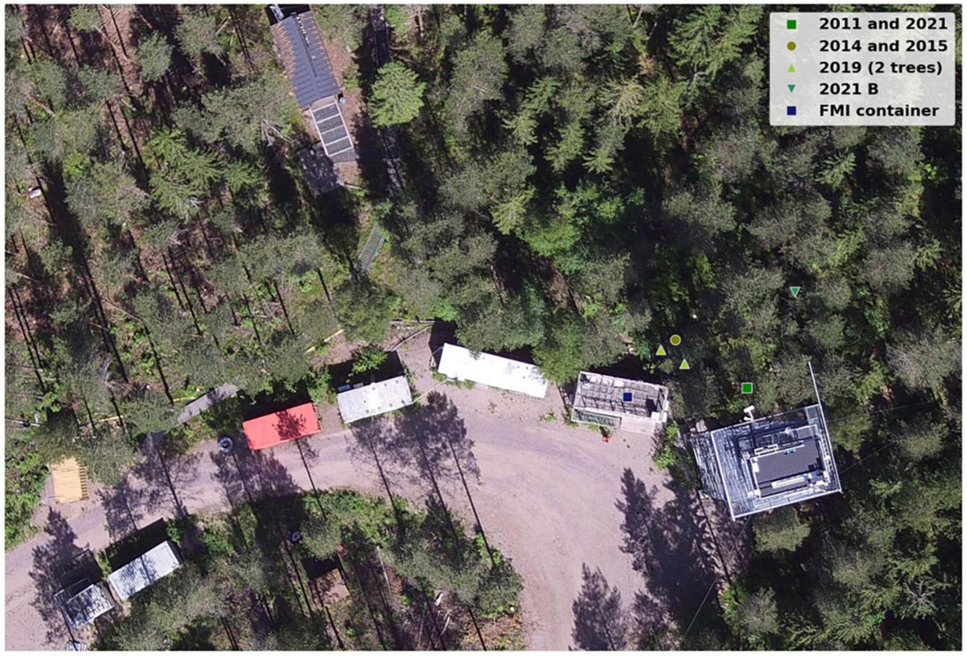
Measurement site in Hyytiälä with the measured Norway spruce trees marked. Picture: Pavel Alekseychik (National Resources Institute Finland), using a Zenmuse XT2 camera (RGB sensor) on a Matrice 210 V2 drone.
2.1.2. Measurement methods
The emission measurement setup used in these campaigns has previously been described in detail, e.g., in Hakola et al. (2017). Briefly, the measurements used a branch enclosure consisting of a ca. 6 L fluorinated ethylene propylene (FEP) dynamic chamber, which was flushed with 3–6 L min–1 of humidified zero air generated by a commercial catalytic converter (HPZA-7000, Parker Hannifin Corporation). Two custom-built data loggers were used during the campaigns. The set-up consisted of a thermistor (Philips KTY 80/110, Royal Philips Electronics, Amsterdam, Netherlands) for the temperature inside the chamber and a quantum sensor (LI-190SZ, LI-COR, Biosciences, Lincoln, USA) for the photosynthetically active radiation (PAR), measured just above the enclosure.
On-line measurements/in situ analysis was performed using a thermal desorption – gas chromatograph – mass spectrometer (TD-GC-MS) (a thermal desorption unit Turbo Matrix 350, a gas chromatograph Clarus 680 and a mass spectrometer Clarus SQ8 T, all manufactured by Perkin-Elmer, Inc. Waltham, MA, USA). It was connected to the chamber via a 7 m-long, 3.2 mm (i.d.) tubing heated a few degrees above the ambient temperature and pumped with 0.5–2.0 L min–1 make up flow, followed by 2.5 m long, 1.59 mm (i.d.) tube, with a flow of 40 mL min–1. All tubing was made of FEP. The VOC samples were collected directly into a trap filled with Tenax TA (50%) and Carbopack B (50%) of the TD-GC-MS for 30 min every hour or every second hour. The trap was kept at 20–25°C during sampling to prevent water vapor present in the air from accumulating in the trap. A DB-5MS column (60 m; i.d., 0.25 mm; film thickness, 0.25 μm from Agilent Technologies, Santa Clara, CA, USA) was used for the separation. The column was kept for 2 min at 60°C and then heated at the rate of 8°C min–1 to 270°C, at which it was kept for 2 min. The total time of the analysis was 30.25 min.
Helin et al. (2020) detected significant losses of β-farnesene within our in situ TD-GC-MSs, which have been used in earlier studies of Norway spruce emissions (Hakola et al., 2017). For the new measurement campaigns conducted in 2019–2021 and presented here, the instrument was modified by changing the stainless steel lines in the online sampling box of the TD unit into FEP tubing and by using an empty Silcosteel sorbent tube instead of an empty stainless steel sorbent tube in the sample path of the TD unit. This increased the recovery of β-farnesene from ∼10 to >80%.
Additional offline samples taken in Hyytiälä in 2021 and in Pallas in 2020 and also two previous datasets (NF2 2002 and SF2 2001) were acquired using Tenax TA/Carbopack B adsorbent tubes with the same method. The sampling flow was ∼100 and ∼200 ml min–1 at Hyytiälä and in Pallas, respectively, and the sampling time was 30 min. The adsorbent tube samples, which were stored at 4°C until analysis, were analyzed later in the laboratory of the Finnish Meteorological Institute using an automatic TD unit (TurboMatrix 350) connected to a GC (GC, Clarus 680) coupled to a quadrupole MS (MS, Clarus SQ 8 T), all purchased from PerkinElmer, Inc. (Waltham, MA, USA). This offline TD-GC-MS method is comparable to the online method (see, e.g., Helin et al., 2020).
A four-point calibration was performed using liquid standards in methanol solutions for both on- and off-line measurements. Standard solutions (5 μl) were injected onto adsorbent tubes and then flushed with nitrogen (80–100 mL min–1) for 10 min to remove the methanol. The calibration solution included the following MTs: α-pinene, camphene, β-pinene, 3Δ-carene, p-cymene, 1,8-cineol, limonene, myrcene, terpinolene, and linalool, and the following SQTs: longicyclene, iso-longifolene, β-caryophyllene, β-farnesene and α-humulene. Unknown sesquiterpenes were tentatively identified based on the comparison of the mass spectra and retention indexes (RIs) with NIST mass spectral library (NIST/EPA/NIH Mass Spectral Library, version 2.0). RIs were calculated for all SQTs using RIs of known SQTs and MTs as reference. These tentatively identified SQTs were quantified using response factors of calibrated SQTs having the closest mass spectra resemblance. Isoprene was calibrated using gaseous standard (National Physical Laboratory, 32 VOC mix at 4 ppb level or terpene mix at 2 ppbv level).
2.2. Published emission data used
The published data includes data obtained in Hyytiälä during campaigns in 2011, 2014, and 2015 (Hakola et al., 2017), and two older data sets; one from Sodankylä, Northern Finland and one from Järvenpää, Southern Finland (Hakola et al., 2003). The trees are named NF/SF and the year of the measurements.
Other data included in the analysis is from Bourtsoukidis et al. (2014a,b) and van Meeningen et al. (2017). van Meeningen et al. (2017) reported isoprenoid emissions rates of Norway spruce at seven different sites, distributed from Ljubljana (46°06 N), Slovenia, to Piikkiö (60°23 N), Finland, to study the effect of latitude. Bourtsoukidis et al. (2014b) reported spruce emission measurements from Germany at the Taunus Observatory on top of Kleiner Feldberg. Bourtsoukidis et al. (2014a) also measured spruce emissions in Estonia during autumn. The measurements outside Finland are named according to the measurement site.
2.3. Emission rate and potential calculations
The emission rate (E) is determined as the mass of compound per needle dry weight and per time according to:
Here C2 is the concentration in the outgoing air, C1 is the concentration in the incoming air, and F is the flow rate into the enclosure. The dry weight of the foliage mass (m) was determined by drying the needles and shoots from the enclosure at 75°C for 24 h.
A strong dependence of biogenic VOC emissions on temperature has been seen in emission studies of ISOP, MTs, and SQTs (e.g., Hellén et al., 2021). The temperature dependent emission potentials for MTs and SQTs were calculated according to Guenther et al. (1993) and isoprene emission potentials were calculated using the temperature and light dependent algorithm according to Guenther et al. (2012).
2.4. Modeling impact of VOC emissions on aerosol formation and growth
Simulations were conducted using the 0D model presented in Taipale et al. (2022). This model includes modules for emissions of VOCs from stress-free and stressed trees, boundary layer meteorology, atmospheric chemistry, and aerosol formation and growth. The model is programmed in Fortran and the time step for each module is 60 s. The model was simulating 1 day at a time and 1 day during every month. The individual processes included in the model are aimed to imitate the mechanistic understanding of those processes. The descriptions of several of the individual processes have been evaluated separately in previous studies (references provided in the subsections below). The model’s ability to reproduce canopy scale emissions of VOCs and the influence of organic compounds on aerosol formation and growth in a Scots pine forest has furthermore been tested by constraining and validating the model with observations from the SMEAR II station (the Station for Measuring Ecosystem-Atmosphere Relations II) in Hyytiälä, Finland Taipale et al. (2022). Certain parts of the model setup used in this study are different from the setup described in Taipale et al. (2022).
2.4.1. Plant emissions of volatile organic compounds
In this study, the emissions (Ei, μg m–2h–1) of MTs and SQTs (i) were modeled as:
where εi (μg m–2h–1) is the emission potential of i, LAI (m2 m–2) is the one-sided leaf area index, and γi (unit-less) is an activity factor which accounts for changes in standard temperature conditions (Guenther et al., 1993):
where T is temperature (°C), Ts is the standard temperature (30°C), and βi is 0.1°C–1 and 0.17°C–1 for monoterpenes and sesquiterpenes, respectively (Guenther et al., 2012). The emission potentials have been converted from ng gdw–1h–1 to μg m–2h–1 assuming a specific (one-sided) leaf weight of 0.15 kg m–2.
2.4.2. Environmental conditions and atmospheric chemistry
The model was constrained by environmental and atmospheric values observed in Hyytiälä (Southern Finland, SF), as well as Pallas and Värriö, (Northern Finland, NF), due to data availability (Figure 3). The aim was to use reasonable values and not simulate one specific year or location. The one-sided leaf area index of Norway spruce forest stands was fixed to 6.0 m2 m–2 (Kalliokoski et al., 2020) and 3.3 m2 m–2 (Thum et al., 2008) for Southern Finland and Finnish Lapland, respectively. In the simulations the concentration of ozone (O3) was kept constant throughout the day For simulations of Lapland, we used monthly median year 2020 O3 concentration data from Pallas Sammaltunturi obtained via EBAS. These values are almost identical to observations from SMEAR I, Värriö, during the same period.1 For simulations of Southern Finland, we used monthly median year 2020 O3 concentration data from SMEAR II, measured at 16.8 m.2 For simulations of both environments we calculated the monthly median of daily maximum OH concentration using the proxy presented by Petäjä et al. (2009) and 2020 observed UVB radiation from the SMEAR I (see text footnote 1) and SMEAR II (see text footnote 2) stations, respectively. These daily maximum OH concentrations were used as input to the model, and the concentration of OH then decreased in the model as a function of a decrease in available solar light. We used daily maximum sulfuric acid (H2SO4) concentrations reported by Asmi et al. (2011) and Kyrö et al. (2014) from Lapland, and by Petäjä et al. (2009) from Southern Finland, as input to the model, and let the concentration of sulfuric acid decrease as a function of a decrease in solar light. In the simulations, the condensation sink (CS) was kept constant throughout the day. For Lapland simulations, we used CS data from Komppula et al. (2006), Asmi et al. (2011), and Vana et al. (2016), while we used CS data from Vana et al. (2016) for Southern Finland simulations. For simplicity, the daily modeled temperature pattern followed that of the solar zenith angle with a forward shift of 1 h. For simulations of both environments, we used the monthly median of daily maximum and minimum temperatures measured at 15 m (Lapland) and 16.8 m (Southern Finland) during 2020 at the SMEAR I (see text footnote 1) and SMEAR II (see text footnote 2) stations. For simulations of both environments, we used the monthly median of daily maximum 2020 ERA5 reanalysis boundary layer height retrieved for the grid cells closest to Pallas and Hyytiälä, respectively. These maximum values were downscaled by 25% since one fixed value was used for the whole day.
FIGURE 3

Model input. (A) Ozone concentration. (B) Daily maximum OH concentration. (C) Daily maximum sulfuric acid concentration. (D) Condensation sink. (E) Daily maximum and minimum temperatures. (F) Planetary boundary layer height (BLH).
The following chemical reactions were included in the model:
OH + MTs → products + γOxOrg(g) (R1)
O3 + MTs → products + γOxOrg(g) (R2)
O3 + SQTs → products+ γOxOrg(g) (R3)
OxOrg(g) → OxOrg(p) (R4)
OH + SO2 → H2SO4(g) (R5)
H2SO4(g) → H2SO4(p) (R6)
where p indicates particle phase, g indicates gas phase, and OxOrg is the sum of all organic compounds that contribute to aerosol processes. Reaction rates for each reaction are summarized in Table 1. Reactions with NO3 were omitted, because simulations were only conducted for daytime conditions.
TABLE 1
| Reaction | Reaction rate | Yield (%) |
| R1 | 1.2⋅10–11⋅e(440/T) (cm3⋅molecule–1⋅s–1) | 1.7 |
| R2 | 8.05⋅10–16⋅e(–640/T) (cm3⋅molecule–1⋅s–1) | 5.0 |
| R3 | 1.2⋅10–14 (cm3⋅molecule–1⋅s–1) | 7.7 |
| R4 | CS⋅0.5 | |
| R5 | 1.5⋅10–12 (cm3⋅molecule–1⋅s–1) | |
| R6 | CS |
Reaction rates and yields for the reactions 1–6.
T is temperature (K) and CS is the condensation sink.
Some VOCs, and especially VOCs with endocyclic double bonds, can undergo autoxidation (Crounse et al., 2013; Ehn et al., 2014) whereby compounds with low volatility and high molecular mass (HOM: highly oxygenated organic molecules) are formed (e.g., Ehn et al., 2012, 2014; Jokinen et al., 2015; Berndt et al., 2016; Kürten et al., 2016; Bianchi et al., 2019; Zhao et al., 2021). These highly oxygenated organic molecules have been found to be a major component of secondary organic aerosol (e.g., Ehn et al., 2014; Mutzel et al., 2015; Tröstl et al., 2016; Roldin et al., 2019). The yields by which HOM are formed are specific for individual parent molecules and isomers (e.g., Ehn et al., 2014; Bianchi et al., 2019), but they also depend on the blend of atmospheric molecules, including VOCs (McFiggans et al., 2019). Since HOM yields have, until now, only been determined for a very limited selection of VOCs, and since no algorithm to quantify how the concentration blend affects HOM yields have been proposed so far, mono- and sesquiterpenes were treated as groups of compounds in the model. Thus, in R1-3, γ is either the reported HOM yield, as defined in Ehn et al. (2014), or the reported SOA yield divided by 2.2 to account for the fact that SOA yields represent mass yields, and not molar yields as it is the case of HOM yields (Ehn et al., 2014). SOA yields were used in addition to HOM yields since HOM yields do not exist for all considered reactions. γ1 is based on Jokinen et al. (2015) and Berndt et al. (2016), γ2 is based on Ehn et al. (2014) and Jokinen et al. (2015), while γ3 is based on Mentel et al. (2013).
All equations related to formation and growth of particles are found in Taipale et al. (2022).
3. Results
3.1. Previously unpublished emission rates
The full time series of unpublished Norway spruce emission rates of MTs, oxygenated monoterpenoids (OMTs: linalool, 1,8-cineol, and bornylacetate) and SQTs are shown in Appendix Figure 1 and isoprene and MBO emission rates in Appendix Figure 2. Calculated monthly mean emission potentials (30°C) are presented in Table 2 together with previously published data. The approximate ages of the trees are shown in Table 2.
TABLE 2
| Tree | Tree age, years | Time | β (MT) | β (SQT) | ISOP | MT | OMT | SQT | References |
| NF2 2002 | >80 | This publication | |||||||
| 67.25°N | April, 2002 | 0.1 | 0.17 | 480 ± 150 | 460 ± 60 | 130 ± 30 | 0 | ||
| May, 2002 | 0.1 | 0.17 | 2470 ± 1460 | 730 ± 440 | 180 ± 100 | 100 ± 130 | |||
| June, 2002 | 0.1 | 0.17 | 7140 ± 1540 | 2130 ± 1150 | 260 ± 110 | 260 ± 110 | |||
| NF 2020 | >80 | This publication | |||||||
| 67.59°N | April, 2020 | 0.1 | 0.17 | 19 ± 20 | 450 ± 220 | 16 ± 8 | 65 ± 27 | ||
| May, 2020 | 0.1 | 0.17 | 26 ± 18 | 90 ± 49 | 7 ± 2 | 368 ± 160 | |||
| June, 2020 | 0.1 | 0.17 | 66 ± 93 | 595 ± 605 | 52 ± 53 | 2260 ± 2680 | |||
| July, 2020 | 0.1 | 0.17 | 76 ± 69 | 400 ± 380 | 150 ± 130 | 1240 ± 1370 | |||
| August, 2020 | 0.1 | 0.17 | 64 ± 80 | 340 ± 400 | 65 ± 80 | 2620 ± 2080 | |||
| NF 2020 R (road side) | >80 | This publication | |||||||
| Adsorbent tubes. New growth only | July, 2020 | 0.1 | 0.17 | 192 ± 113 | 36 ± 22 | 99 ± 68 | |||
| NF 2020 F (forest) | >80 | This publication | |||||||
| Adsorbent tubes. New growth only | July, 2020 | 0.1 | 0.17 | 12 ± 8 | 2900 ± 1830 | 420 ± 240 | 790 ± 500 | ||
| SF 2011 | 40 | Hakola et al., 2017 | |||||||
| 61.51° N | April, 2011 | 0.1 | 0.17 | 0 | 49 ± 91 | 10 ± 6 | da | ||
| May, 2011 | 0.1 | 0.17 | 120 ± 160 | 19 ± 13 | 5 ± 3 | da | |||
| June, 2011 | 0.1 | 0.17 | 3 ± 2 | 40 ± 42 | 13 ± 10 | da | |||
| SF 2014 | 33–40 | Hakola et al., 2017 | |||||||
| May, 2014 | 0.1 | 0.17 | 80 ± 30 | 3 ± 2 | da | ||||
| June, 2014 | 0.1 | 0.17 | 41 ± 34 | 13 ± 19 | da | ||||
| July, 2014 | 0.1 | 0.17 | 78 ± 22 | 6 ± 5 | da | ||||
| SF 2015 | 33–40 | Hakola et al., 2017 | |||||||
| Same tree as 2014 | June, 2015 | 0.1 | 0.17 | 160 ± 310 | 130 ± 200 | 33 ± 45 | da | ||
| July, 2015 | 0.1 | 0.17 | 33 ± 20 | 160 ± 70 | 41 ± 23 | da | |||
| August, 2015 | 0.1 | 0.17 | 180 ± 920 | 60 ± 38 | 18 ± 18 | da | |||
| SF 2019 | 33–40 | This publication | |||||||
| June, 2019 | 0.1 | 0.17 | 13 ± 36 | 29 ± 25 | 37 ± 45 | 42 | |||
| July, 2019 | 0.1 | 0.17 | 14 ± 42 | 58 ± 99 | 34 ± 36 | 34 | |||
| August, 2019 | 0.1 | 0.17 | 11 ± 12 | 21 ± 29 | 14 ± 11 | 118 | |||
| September, 2019 | 0.1 | 0.17 | 43 ± 46 | 21 ± 7 | 2330 | ||||
| SF 2021 | 50 | This publication | |||||||
| Same tree as 2011 | August, 2021 | 0.1 | 0.17 | 1 ± 4 | 32 ± 49 | 10 ± 17 | 2170 ± 2170 | ||
| September, 2021 | 0.1 | 0.17 | 0 | 24 ± 12 | 7 ± 5 | 13700 ± 6100 | |||
| SF 2021 B | 50 | This publication | |||||||
| Adsorbent tubes | July, 2021 | 0.1 | 0.17 | 2060 ± 1720 | 280 ± 450 | 65 ± 67 | 1030 ± 1440 | ||
| August, 2021 | 0.1 | 0.17 | 1181 ± 842 | 53 ± 29 | 3 ± 3 | 114 ± 34 | |||
| SF2 2001 | >100 | Hakola et al., 2003 | |||||||
| Adsorbent tubes | Spring 2001 | 0.1 | 0.17 | 490 ± 380 | 410 ± 850 | 55 ± 35 | 8 ± 24 | ||
| 60.28°N | Summer 2001 | 0.1 | 0.17 | 950 ± 1380 | 640 ± 710 | 52 ± 68 | 230 ± 360 | ||
| Autumn 2001 | 0.1 | 0.17 | 640 ± 750 | 230 ± 260 | 8 ± 23 | 59 ± 88 | |||
| Järvselja, Estonia | Big tree | Bourtsoukidis et al., 2014a | |||||||
| 58.27°N | Autumn 2012 | 0.10 ± 0.02 | 0.13 ± 0.04 | Low | 540 ± 63 | 113 ± 19 | |||
| Taunus mountains | 60–80 | Bourtsoukidis et al., 2014b | |||||||
| Germany | Spring 2011 | 0.14 ± 0.02 | 0.09 ± 0.01 | Low | 2837 ± 369 | 534 ± 534 | |||
| 50.22°N | Summer 2011 | 0.12 ± 0.02 | 0.12 ± 0.02 | Low | 978 ± 141 | 353 ± 56 | |||
| Autumn 2011 | 0.08 ± 0.01 | 0.11 ± 0.01 | Low | 356 ± 66 | 176 ± 62 | ||||
| Ljubljana, Slovenia, 46°04 | 54 | April–May | 310 ± 290 | 1170 ± 1460 | 500 ± 1280 | van Meeningen et al., 2017 | |||
| Grafrath, Germany, 48°18 | 51–53 | June | 640 ± 920 | 1600 ± 1240 | 100 ± 290 | van Meeningen et al., 2017 | |||
| Taastrup, Denmark, 55°40 | 43–45 | July | 510 ± 780 | 1960 ± 1950 | 330 ± 840 | van Meeningen et al., 2017 | |||
| Hyltemossa, Sweden, 56°06 | 30 | July | 430 ± 120 | 1250 ± 1140 | 340 ± 380 | van Meeningen et al., 2017 | |||
| Skogaryd, Sweden, 58°23 | 53 | October | 110 ± 610 | 290 ± 250 | n.d. | van Meeningen et al., 2017 | |||
| Norunda, Sweden, 60°05 | 119 | June | 3790 ± 3480 | 1510 ± 1190 | 230 ± 200 | van Meeningen et al., 2017 | |||
| Piikkiö, Finland, 60°23 | 49 | July | 100 ± 80 | 1470 ± 1520 | 170 ± 190 | van Meeningen et al., 2017 |
Mean monthly emission potentials (30°C) from the present study and from literature (ng g–1(dw) h–1), average ± standard deviation.
da, degraded in the analysis. van Meeningen et al. (2017) reported measurements from several heights, 1–2 m measurements are included here, since they best correspond to our measurements. For Norunda, Sweden, the height is 3 m and Järvselja, Estonia 16 m. β is the coefficient describing temperature dependence according to Eq. 3.
3.1.1. Emission rates in Southern Finland
In 2019, emissions from a small, 33–40-year-old tree (SF 2019) were measured during the growing season. It emitted only small amounts of ISOP, and MT and SQT emissions were generally lower than in the previously reported Norway spruce emissions (Hakola et al., 2003). The statistics of the daily mean emission rates are shown in Figure 4. Figure 5 shows the mean diurnal variations during summer months. Diurnal variation of the emission rates followed the variation of the temperature being highest in the afternoon and very low or below detection limits during the night. Isoprene emission rates were very low all the time. MTs were the dominant group in the emissions in July, but SQT were also important throughout the summer.
FIGURE 4
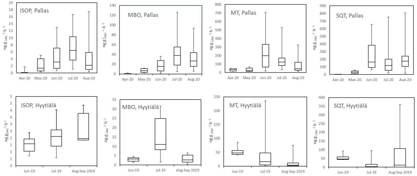
Monthly box and whisker plots of ISOP, MBO, MT, and SQT calculated from daily mean emission rates of trees in Pallas in 2020 (NF 2020) and in Hyytiälä in 2019 (SF 2019). Boxes represent second and third quartiles and horizontal lines in the boxes median values. Whiskers show the highest and the lowest daily means.
FIGURE 5
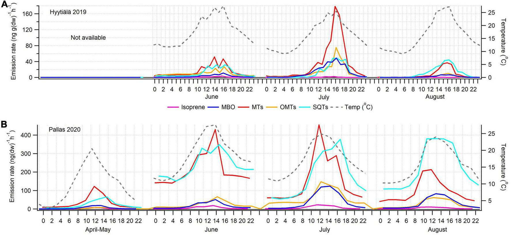
Mean diurnal variations of isoprene, MBO, MTs, OMTs, and SQTs in (A) Hyytiälä 2019 and (B) Pallas 2020 together with temperature in the enclosure.
The tree measured in Hyytiälä in 2021 (SF 2021) was the same one that was measured in 2011 (SF 2011). In 2011, the SQT measurements were not reliable, but otherwise the results remained similar after ten years with very low ISOP, MT, and OMT emission potentials (Table 2). The comparison between the years is difficult since the measurements are not from the same periods in 2011 and 2021. In 2021 the measurements were conducted in late summer (August), whereas in 2011 they were done in spring/early summer. Based on these measurements, the aging of the tree did not affect the emissions, at least not up that point during the ten-year period. In 2021, an additional big tree growing deeper in the forest was measured (SF2021B) for comparison. SF2021 and SF2021B were both about 50 years old in 2021, but their emission potentials were very different. In August SF2021B emitted isoprene at a much higher rate than SF2021 and the small trees (mean 1498 ng gdw–1h–1) and its MT emission rates (mean 178 ng gdw–1h–1) were also higher. On the other hand, SF2021 emitted much more SQTs (Table 2).
Sesquiterpene emissions were substantial compared to ISOP and MT emissions in all trees in Hyytiälä. The most noteworthy thing is that SQT emission rates greatly increased at the end of the growing season both in 2019 and 2021 (Figure 4). For tree SF 2021, the emission rates increased a lot and the highest rates reached 1.5 μg gdw–1h–1 (Appendix Figure 1). The emissions followed the typical diurnal variation, with highest emissions in the afternoon and lowest during the night (Figure 5). The main identified SQT was β-farnesene, but a significant fraction of the SQTs remained unidentified (Table 2). One of the major unidentified SQTs was tentatively identified as α-farnesene.
3.1.2. Emission rates in Northern Finland
At Pallas one big tree was measured with the in situ TD-GC-MS in April-August 2020 (NF 2020) and two additional big trees were measured using adsorbent tubes in July 2020, one of them was growing by the roadside (NF 2020R) and the other deeper in the forest (NF 2020F). In these additional measurements, only new growth was measured.
Average emission rates of ISOP, MTs and SQTs from the main tree (NF 2020) were 7, 135 and 230 ng gdw–1h–1, respectively. At the time of high emissions, in summer, SQTs were the most significant compounds group emitted (Table 2 and Figure 4), although in spring when the emissions were quite low, MTs dominated. Whereas SQT emissions in Southern Finland were highest at the end of growing season, in Northern Finland they were already high in June. Diurnal variations of all emitted compounds followed the variations of temperature, as expected (Figure 5). Significant emissions of MTs and SQTs were also detected during at night, while emissions of ISOP and MBO decreased close to or below detection limits. ISOP and MBO emissions are known to be light dependent (Guenther, 1997; Harley et al., 1998) and even though there is midnight sun at this sub-Arctic site in summer, PAR decreased down to <10 μmol s–1 m–2 in the middle of the night.
The emissions of the main tree and two additional trees with new growth measurements differed a lot. The additional tree growing deeper in the forest (NF 2020F) emitted about 10 times more MTs than the other two trees, and SQT emission rates were also higher (Table 2). We have no explanation for this difference. ISOP emissions were very low all the time from all trees. The branches were searched for possible diseases, but nothing was found. However, all three trees in Pallas had rather similar emission compositions (Table 3). β-farnesene was the dominant SQT and other abundant compounds were α-pinene, β-pinene, limonene and Δ3-carene.
TABLE 3
| SF 2019 | SF 2019 | SF 2019 | SF 2021 | SF 2021 | SF 2021B | SF2021B | NF 2020 | NF 2020 | NF 2020 | NF 2020 | NF 2020 | NF 2020F | NF 2020R | |
| June | July | August | August | September | July | August | April | May | June | July | August | July | July | |
| Isoprene | 1 | 0 | 0 | 0 | 0 | 72 | 85 | 0 | 3 | 1 | 2 | 1 | 0 | 0 |
| MBO | 12 | 18 | 4 | 1 | 0 | 2 | 4 | 1 | 9 | 3 | 10 | 8 | 0 | 0 |
| MT | 0 | 0 | 0 | 0 | 0 | 0 | 0 | 0 | 0 | 0 | 0 | 0 | 0 | 0 |
| α-pinene | 7 | 4 | 3 | 1 | 0 | 2 | 2 | 13 | 16 | 11 | 10 | 5 | 15 | 14 |
| β-pinene | 5 | 3 | 1 | 0 | 0 | 1 | 0 | 10 | 3 | 7 | 4 | 3 | 12 | 7 |
| Camphene | 2 | 4 | 3 | 0 | 0 | 1 | 0 | 4 | 6 | 4 | 5 | 2 | 14 | 13 |
| Carene | 4 | 2 | 0 | 0 | 0 | 2 | 0 | 14 | 4 | 6 | 3 | 4 | 20 | 14 |
| Limonene | 16 | 32 | 12 | 1 | 0 | 1 | 0 | 17 | 7 | 7 | 5 | 5 | 10 | 11 |
| Myrcene | 1 | 2 | 1 | 1 | 0 | 1 | 0 | 25 | 2 | 4 | 2 | 2 | 0 | 0 |
| β-phellandrene | 0 | 0 | 0 | 0 | 0 | 0 | 0 | 7 | 2 | 2 | 2 | 1 | 0 | 0 |
| Sabinene | 1 | 1 | 1 | 0 | 0 | 0 | 0 | 0 | 1 | 1 | 1 | 0 | 0 | 0 |
| Terpinolene | 0 | 0 | 0 | 0 | 0 | 0 | 0 | 3 | 1 | 1 | 0 | 1 | 1 | 2 |
| MT total | ||||||||||||||
| OMT | ||||||||||||||
| 1,8-cineol | 16 | 14 | 5 | 1 | 0 | 0 | 0 | 1 | 1 | 0 | 3 | 1 | 8 | 7 |
| Linalool | 3 | 3 | 0 | 1 | 0 | 2 | 0 | 2 | 0 | 2 | 5 | 4 | 2 | 6 |
| Bornylacetate | 0 | 1 | 0 | 0 | 0 | n.a. | n.a. | 1 | 1 | 2 | 4 | 1 | 6 | 5 |
| OMT total | ||||||||||||||
| SQT | ||||||||||||||
| Iso-longifolene | 0 | 0 | 0 | 0 | 24 | 0 | 0 | 0 | 0 | 0 | 0 | 0 | 0 | 0 |
| β-farnesene | 17 | 7 | 26 | 46 | 0 | 11 | 4 | 1 | 18 | 35 | 35 | 41 | 11 | 20 |
| β-caryophyllene | 10 | 7 | 0 | 0 | 0 | 0 | 0 | 0 | 0 | 0 | 0 | 0 | 0 | 0 |
| A-humulene | 0 | 0 | 0 | 0 | 21 | 0 | 0 | 0 | 0 | 0 | 0 | 0 | 0 | 0 |
| Unidentified SQTs | 4 | 1 | 43 | 47 | 54 | 5 | 3 | 1 | 23 | 13 | 9 | 19 | 0 | 0 |
| SQT total | ||||||||||||||
| Emission (ng g(dw)–1 h–1) | 53 | 79 | 38 | 210 | 841 | 2082 | 499 | 36 | 68 | 474 | 449 | 452 | 1721 | 144 |
| Number of measurements | 144 | 392 | 326 | 193 | 109 | 23 | 10 | 46 | 74 | 246 | 468 | 297 | 10 | 10 |
Contributions (%) of the most abundant compounds in the emissions of Norway spruce in Northern and Southern Finland trees.
The empty cells mean the compound was not detected.
3.2. Comparison of Norway spruce emission potentials
3.2.1. Variations in spruce ISOP emission potentials
The compiled ISOP emission potentials ranged from below the detection limit to 7138 ng gdw–1h–1. No clear link between the emissions potentials and the latitude, or the season could be observed, but none of the smaller trees investigated emitted ISOP. The trees with the largest emissions were NF2 2002, SF2 2001, and SF 2021B, in June and July. Their ISOP emission potentials were larger than the one reported by van Meeningen et al. (2017), except for the tree in Norunda (60°23N), Sweden. While this could indicate that ISOP emission potentials might be higher at higher latitudes, the trees in Northern Finland (NF 2020, NF 2020R, and NF 2020F) and in Southern Finland (SF 2019 and SF 2021) and reported by Bourtsoukidis et al. (2014a,b) also exhibited low ISOP emission potentials. According to our observations, latitude is not a main driver for variations in emission potentials, which is also in accordance with van Meeningen et al. (2017) who found only minimal differences in emission potentials between sites and across latitudes. van Meeningen et al. (2017) studied the effects of branch height and season, and variation between years on observed emission patterns was also investigated. There were indications of potential influences of all three factors. However, due to different experimental setups between measurement campaigns, it was difficult to draw any robust conclusions. The effect of branch height has not been explicitly studied in our campaigns as only the lowest branches were measured.
3.2.2. Variation in MT emission potentials
We found larger variations of MT emission potentials (9–2909 ng g(dw)–1h–1) compared to Bourtsoukidis et al. (2014a,b), and van Meeningen et al. (2017), again with no clear trend with changes in latitude. Even for the summer months (June to August), the variations were large (39–2909 ng gdw–1h–1). Here, it seems that, in general, younger trees (less than 80 years old) had lower MT emission potentials (9–1960 ng g(dw)–1h–1), compared to older trees (91–2909 ng g(dw)–1h–1), with a large overlap of values. Whenever seasonal data is available, MT emission potentials were higher in spring and summer. This confirms the findings of Bourtsoukidis et al. (2014a), in which the highest MT (977.5 ± 140.7 ng gdw–1h–1) emission potentials were detected during spring with a decline toward autumn.
3.2.3. Variation in OMT emission potentials
Bourtsoukidis et al. (2014a,b) and van Meeningen et al. (2017) did not report OMT emission potentials separately. In our studies emission potentials of OMTs have ranged from below the detection limit to 19 ng gdw–1h–1. The largest emission potentials were found in July for trees NF 2020F, NF2 2002, and NF 2020.
3.2.4. Variation in SQT emission potentials
As was shown in Helin et al. (2020), the SQT measurements in Southern Finland in 2011 and 2014 (Hakola et al., 2017) were underestimated, since β-farnesene, usually the main SQT emitted from Norway spruce, was degraded during the analysis. The SQT emission potentials from 2011 to 2014 are therefore not shown in Table 2. The SQT emissions potentials based on the rest of our measurement campaigns varied between below the detection limit and 13664 ng gdw–1h–1 (between 34 and 3243 ng gdw–1h–1 for the summer months). Bourtsoukidis et al. (2014a) reported highest SQT emission potentials in spring (352.9 ± 56.1 ng gdw–1h–1), declining toward autumn, similarly to MT emission potentials from the same study. All our measurements that continued until late summer/early autumn have different trends, with increasing emission potentials toward the end of the growing season (Table 2). Table 4 shows the mean values of emission potentials of the trees measured in Finland (this study and older data) and the standard deviation between the trees is presented. We did not take into account the results of Bourtsoukidis et al. (2014a,b) or van Meeningen et al. (2017), because the standardization was not done with the same β values and the ages of the trees in the measurements by Bourtsoukidis et al. (2014a) was not reported.
TABLE 4
| >80 years | ISOP | MT | OMT | SQT |
| Spring (3) | 700 ± 740 | 390 ± 111 | 80 ± 72 | 110 ± 120 |
| Summer (5) | 1200 ± 3900 | 1000 ± 840 | 190 ± 110 | 1100 ± 1100 |
| Autumn (1) | 910 | 140 | 7 | 90 |
| <80 years | ISOP | MT | OMT | SQT |
| Spring (3) | 60 | 40 | 8 | Na |
| Summer (6) | 370 ± 710 | 90 ± 60 | 30 ± 10 | |
| Summer (2) SQT | 1300 ± 1100 | |||
| Autumn (2) | bdl | 16 ± 11 | 4 ± 4 | 8000 ± 8010 |
Mean values of emission potentials for the trees (>80 and <80 years) measured in Finland (this study and older data) and the standard deviation between the trees.
N = the number of trees measured each season is given in parentheses. Bdl, below detection limit; Na, not available.
3.2.5. Overall conclusion of the comparison
van Meeningen et al. (2017) concluded that spruce isoprenoid emissions are potentially more determined by genetic diversity than by adaptation to local growth conditions. This conclusion is holding up in view of the review performed here, even though weak trends could be identified regarding the age and size of the trees.
Generally, we found that older trees (>80 years) emit more isoprene and MT than younger trees (<80 years) However, age does not seem to affect SQT emissions. This is reflected in the full review presented here, when comparing mean values of all measured trees older than 80 years and younger than 80 years. The old trees were found to emit about ten times more ISOP and MTs than younger trees (Table 4), while SQT emissions do not seem to vary with the age of the tree. SQT emissions are often related to stress effects, as has been suggested in many studies (e.g., Petterson, 2007; Kännaste et al., 2008; Niinemets, 2010; Joutsensaari et al., 2015; Matsui and Koeduka, 2016).
While we found some indication that smaller trees have lower emission potentials, all the small trees measured were growing in Hyytiälä, so this could also be due to the same genetic origin. Big trees can be divided into two groups: three trees growing in NF emitted considerable amounts of MTs and SQTs, but small amounts of isoprene [like the trees measured in Estonia and Germany by Bourtsoukidis et al. (2014a,b) and big trees growing in SF and one growing in NF additionally emitted lots of isoprene].
4. Impact of Norway spruce emissions on aerosol formation and growth
Recognizing this observed large variability in spruce BVOC emissions (precursors for new particle formation processes), there is a need to test the consequences of this variability in simulations of aerosol formation. For Southern Finland (SF) spruce forest emission potentials obtained from Hyytiälä were used, while for Northern Finland (NF) emission potentials obtained from Pallas were used. As a comparison, simulations were also conducted using standard emission potentials for needleleaf evergreen boreal trees from MEGAN v2.1. Simulations were run first by including all measured compounds and then either MT or SQT emissions were set to zero to study the relative impacts of MTs and SQTs.
The emission potentials used in the simulations are listed in Table 5. ISOP was excluded from model simulations, since previous measurements as well as the measurements presented in this paper show that the emission of ISOP from Norway spruce is negligible or very low most of the time. Furthermore, the emission factor for ISOP for needleleaf evergreen boreal tree in MEGAN is very high (600 μg m–2h–1 for a one-sided LAI of 1 m2 m–2, Guenther et al., 2012), due to the high emission of ISOP from other tree species within the same plant functional type (Guenther et al., 2012). Additionally, the role of ISOP in aerosol formation and growth processes is unclear. ISOP has a small HOM yield (∼0.01–0.03%, Jokinen et al., 2015) and it has been suggested that it suppresses the formation of new particles (Kiendler-Scharr et al., 2009, 2012; Lee et al., 2016; McFiggans et al., 2019; Heinritzi et al., 2020). On the other hand, oxidation products of ISOP (e.g., IEPOX) have been proposed to promote the growth of existing new particles (Dp > 3 nm, e.g., Surratt et al., 2010; Lin et al., 2013), while others have found the growth of small particles (Dp > 3.2 nm) to be unaffected by the concentration of ISOP (Heinritzi et al., 2020).
TABLE 5
| Southern Finland, 2019a | Northern Finland, 2020a | MEGAN v2.1b | ||||
| MT | SQT | MT | SQT | MT | SQT | |
| April | 72 | 13 | 290 | 48 | ||
| May | 15 | 56 | 290 | 48 | ||
| June | 14 | 17 | 97 | 342 | 290 | 48 |
| July | 32 | 81 | 81 | 189 | 290 | 48 |
| August | 10 | 66 | 61 | 408 | 290 | 48 |
| September | 13 | 384 | 290 | 48 | ||
Emission potentials (μg m–2h–1) used in the simulations.
aThe values have been converted from ng gdw–1h–1 (shown in Table 2) to μg m–2h–1 assuming a specific (one-sided) leaf weight of 0.15 kg m–2.
bNeedleleaf evergreen boreal tree, the values have been decreased by a factor of 5, accounting for the fact that emission factors in MEGAN are standardized to a one-sided LAI of 5 m2 m–2.
MT, monoterpenes, including oxygen-containing monoterpenes; SQT, sesquiterpenes.
Our data indicates that the Norway spruce dominated forests, especially in Northern Finland, are expected to have much higher SQT emissions than predicted by the standard emission potentials for needleleaf evergreen boreal tree in MEGAN 2.1. On the other hand, the ISOP and MT emission potentials obtained from our measurements are lower than those used in MEGAN v2.1. This can have significant impacts on predictions of formation and growth of new particles as shown in our model simulations.
According to our modeling efforts, oxidation products of primary BVOC emissions from spruce contribute significantly more to aerosol processes in Northern Finland than in Southern Finland. In the simulations of Southern Finland, the sum of organic compounds contributing to aerosol processes (OxOrg) is 65% smaller when using the emission potentials obtained from Hyytiälä compared to when using emission factors from MEGAN (Figure 6A). Using either emission potentials obtained from Pallas or from MEGAN achieved comparable results when simulating Northern Finland (Figure 6A). Simulations conducted with and without MTs and SQTs showed that SQTs are the main contributors to OxOrg production in both Southern and Northern Finland when emission potentials obtained from Hyytiälä and Pallas are used, while MTs are the main contributors when emission factors from MEGAN are instead used (Figure 6A). The dominance of SQTs is also displayed in the formation rate of new particles (Figure 6B), the number of newly produced particles (Figure 6C) and the rate at which they grow (Figure 6D).
FIGURE 6
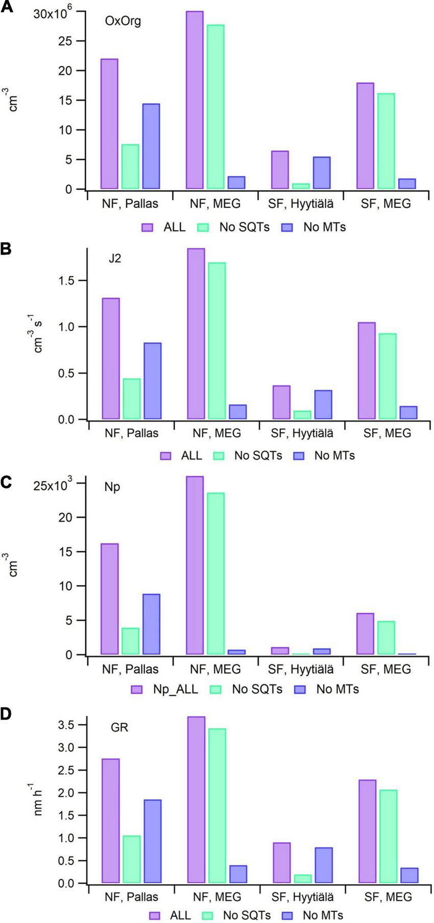
Results from the simulations of the formation and growth of new particles from the emissions of Norway spruce forests in Southern Finland (SF) and in Northern Finland (NF). Mean local emission potentials measured in Hyytiälä and Pallas or standard emission potentials for needleleaf evergreen boreal tree from MEGAN v2.1 (MEG) were used. (A) Sum of oxidation products of MT and SQT emissions contributing to aerosol processes (OxOrg), (B) formation rate of neutral 2 nm-sized clusters (J2), (C) number of new particles in the growing mode (Np), (D) growth rate of newly formed particles (GR). All values are means of monthly medians (June-August). Local environmental conditions are used in all simulations, as described in the method section.
It is possible that spruce SQT emissions have been underpredicted in earlier studies due to difficulties in the quantitative measurements of their emissions. Based on our model simulations, these SQT emissions may have strong impacts on the formation and growth of new particles. However, neither emissions nor atmospheric processes of SQTs are well described, and more research would be needed to better characterize their atmospheric impacts and role in the biosphere-atmosphere interactions especially at Northern latitudes.
5. Conclusion
We studied VOC emissions from eight different Norway spruces growing in Northern and Southern Finland and reviewed the available VOC emission data of Norway spruces measured elsewhere. The outcome was that emissions were highly variable between individual trees. For MT and SQT, differences ∼80 times were found between the emission potentials of the highest and lowest emitting trees in summer. For isoprene the difference was even higher. No clear reason for the differences were found, but there were some indications of the impact of the size/age of the trees and the seasonality of emissions.
We found that none of the younger trees in Hyytiälä emitted isoprene, while one 50-year-old tree growing in Hyytiälä was a strong isoprene emitter. This could perhaps indicate that young Norway spruce trees do not emit isoprene in contrast to older trees, but we cannot confirm this since all measured small trees were growing in Hyytiälä, thus the cause might be that the trees were of the same genetic origin. In addition, at other sites some big trees did not emit significant amounts of isoprene either. On average, older trees (>80 years) emitted about ten times more isoprene and MTs than younger ones (<80 years), but no clear difference was seen in SQT emissions. SQT emissions can be more related to stress effects as has been suggested in many studies (e.g., Petterson, 2007; Kännaste et al., 2008; Niinemets, 2010; Joutsensaari et al., 2015; Matsui and Koeduka, 2016).
It is also significant that SQT emission rates greatly increased at the end of the growing season in all of the measurements conducted in Finland, but in the measurements by Bourtsoukidis et al. (2014b), high SQT emissions were measured during the early growing season. An increase in sesquiterpene emissions toward the late summer has also been seen in Scots pine branches (Tarvainen et al., 2005; Hakola et al., 2006).
With improved measurement methods in this study, we found much higher SQT emissions from Norway spruces than measured before and on average SQTs had higher emission potentials than isoprene and MTs. Due to difficulties in quantitative measurements, SQT emissions from other plant species may also be much higher than earlier thought. As shown here for Norway spruce, if the emission factors of SQTs are in reality higher than what is currently used in models, this may have very significant effects on predictions of aerosol dynamics, including the evolution of aerosol number size distribution via new particle formation and subsequent particle growth. Due to the high SOA formation potentials of SQTs (Griffin et al., 1999; Lee et al., 2006; Frosch et al., 2013; Mentel et al., 2013), the impact on SOA formation and mass could be even higher. Therefore, more studies should focus on quantifying the emission and atmospheric impacts of SQTs.
Statements
Data availability statement
The raw data supporting the conclusions of this article will be made available by the authors, without undue reservation.
Author contributions
HHa: planning the studies. DT: modeling and participate in writing the manuscript. AP and SS: measurements in Hyytiälä and participate in writing the manuscript. ST: measurements in Hyytiälä. TT: measurements at Pallas and in Hyytiälä. AH: analytical method development, measurements at Pallas, and in Hyytiälä. JB: participate in writing the manuscript. HHe: overall responsibility of the measurements, participate in writing the manuscript, and planning the studies. All authors contributed to the article and approved the submitted version.
Funding
This work was financially supported by the Academy of Finland projects (project nos. 316151, 307957, and 337549) and Academy of Finland Postdoctoral Researcher grant (323255) are gratefully acknowledged.
Acknowledgments
We thank Dr. Juho Aalto for determining the tree ages, the needles, and Dr. Pavel Alekseychik (National Resources Institute Finland), for providing us the figure taken using a drone (Figure 2).
Conflict of interest
The authors declare that the research was conducted in the absence of any commercial or financial relationships that could be construed as a potential conflict of interest.
Publisher’s note
All claims expressed in this article are solely those of the authors and do not necessarily represent those of their affiliated organizations, or those of the publisher, the editors and the reviewers. Any product that may be evaluated in this article, or claim that may be made by its manufacturer, is not guaranteed or endorsed by the publisher.
Footnotes
1.^ http://urn.fi/urn:nbn:fi:att:8b3c67b4-22c0-4589-be00-a3d0341064d5
2.^ https://doi.org/10.23729/62f7ad2c-7fe0-4f66-b0a4-8d57c80524ec
References
1
Artaxo P. Hansson H. Andrea M. O. Bäck J. Alves E. G. Barbosa H. M. J. et al (2022). Tropical and boreal forest- atmosphere interactions: a review.Tellus B7424–163.
2
Asmi A. Wiedensohler A. Laj P. Fjaeraa A.-M. Sellegri K. Birmili W. et al (2011). Number size distributions and seasonality of submicron particles in Europe 2008–2009.Atmos. Chem. Phys.115505–5538. 10.5194/acp-11-5505-2011
3
Aurela M. Lohila A. Tuovinen J.-P. Hatakka J. Penttilä T. Laurila T. (2015). Carbon dioxide and energy flux measurements in four northern-boreal ecosystems at Pallas.Boreal Env. Res.20455–473.
4
Bäck J. Aalto J. Henriksson M. Hakola H. He Q. Boy M. (2012). Chemodiversity in terpene emissions in a boreal Scots pine stand.Biogeosciences9689–702.
5
Berndt T. Richters S. Jokinen T. Hyttinen N. Kurtén T. Otkjær R. V. et al (2016). Hydroxyl radical-induced formation of highly oxidized organic compounds.Nat. Commun.7:13677. 10.1038/ncomms13677
6
Bianchi F. Kurten T. Riva M. Mohr C. Rissanen M. P. Roldin P. et al (2019). Highly oxygenated organic molecules (HOM) from gas-phase autoxidation involving peroxy radicals: a key contributor to atmospheric aerosol.Chem. Rev.1193472–3509. 10.1021/acs.chemrev.8b00395
7
Bourtsoukidis E. Bonn B. Dittmann A. Hakola H. Hellén H. Jacobi S. (2012). Ozone stress as a driving force of sesquiterpenes emissions: a suggested parameterization.Biogeosciences94337–4352.
8
Bourtsoukidis E. Bonn B. Noe S. (2014a). On-line field measurements of BVOC emissions from Norway spruce (Picea abies) at the hemiboreal SMEAR-Estonia site under autumn conditions.Boreal Environ. Res.19153–167.
9
Bourtsoukidis E. Williams J. Kesselmeier J. Jacobi S. Bonn B. (2014b). From emissions to ambient mixing ratios: online seasonal field measurements of volatile organic compounds over a Norway spruce-dominated forest in central Germany.Atmos. Chem. Phys.146495–6510. 10.5194/acp-14-6495-2014
10
Cao J. Situ S. Hao Y. Xie S. Li L. (2022). Enhanced summertime ozone and SOA from biogenic volatile organic compound (BVOC) emissions due to vegetation biomass variability during 1981–2018 in China.Atmos. Chem. Phys.222351–2364. 10.5194/acp-22-2351-2022
11
Crounse J. D. Nielsen L. B. Jørgensen S. Kjaergaard H. G. Wennberg P. O. (2013). Autoxidation of organic compounds in the atmosphere.Phys. Chem. Lett.43513–3520. 10.1021/jz4019207
12
Ehn M. Kleist E. Junninen H. Petäjä T. Lönn G. Schobesberger S. (2012). Gas phase formation of extremely oxidized pinene reaction products in chamber and ambient air.Atmos. Chem. Phys.125113–5127. 10.5194/acp-12-5113-2012
13
Ehn M. Thornton J. A. Kleist E. Sipilä M. Junninen H. Pullinen I. et al (2014). A large source of low-volatility secondary organic aerosol.Nature506476–479. 10.1038/nature13032
14
Faiola C. Taipale D. (2020). Impact of insect herbivory on plant stress volatile emissions from trees: a synthesis of quantitative measurements and recommendations for future research.Atmos. Environ: X5:100060. 10.1016/j.aeaoa.2019.100060
15
Frosch M. Bilde M. Nenes A. Praplan A. P. Jurányi Z. Dommen J. et al (2013). CCN activity and volatility of caryophyllene secondary organic aerosol.Atmos. Chem. Phys.132283–2297. 10.5194/acp-13-2283-2013
16
Griffin R. J. Cocker D. R. Flagan R. C. Seinfeld J. H. (1999). Organic aerosol formation from the oxidation of biogenic hydrocarbons.J. Geophys. Res.1043555–3567.
17
Guenther A. (1997). Seasonal and spatial variations in natural volatile organic compound emissions. Ecol. Appl. 7, 34–45.
18
Guenther A. B. Jiang X. Heald C. L. Sakulyanontvittaya T. Duhl T. Emmons L. K. et al (2012). The model of emissions of gases and aerosols from nature version 2.1 (MEGAN2.1): an extended and updated framework for modeling biogenic emissions.Geosci. Model Dev.51471–1492. 10.5194/gmd-5-1471-2012
19
Guenther A. B. Zimmerman P. R. Harley P. C. Monson R. K. Fall R. (1993). Isoprene and monoterpene emission rate variability: model evaluation and sensitivity analyses.J. Geophys. Res.9812609–12617.
20
Hakola H. Laurila T. Lindfors V. Hellén H. Gaman A. Rinne J. (2001). Variation of the VOC emission rates of birch species during the growing season.Boreal Environ. Res.6237–249.
21
Hakola H. Tarvainen V. Bäck J. Rinne J. Ranta H. Bonn B. et al (2006). Seasonal variation of mono- and sesquiterpene emission rates of Scots pine.Biogeosciences393–101.
22
Hakola H. Tarvainen V. Laurila T. Hiltunen V. Hellén H. Keronen P. (2003). Seasonal variation of VOC concentrations above a boreal coniferous forest.Atmos. Environ.371623–1634.
23
Hakola H. Tarvainen V. Praplan A. P. Jaars K. Hemmilä M. Kulmala M. et al (2017). Terpenoid, acetone and aldehyde emissions from Norway spruce.Atmos. Chem. Phys.173357–3370. 10.5194/acp-17-3357-2017
24
Hari P. Kulmala M. (2005). Station for measuring ecosystem-atmosphere relations (SMEAR II).Boreal Env. Res.10315–322.
25
Harley P. Fridd-Stroud V. Greenberg J. Guenther A. Vasconcellos P. (1998). Emission of 2-methyl-3-buten-2-ol by pines: a potentially large natural source of reactive carbon to the atmosphere.J. Geophys. Res.10325479–25486.
26
Heinritzi M. Dada L. Simon M. Stolzenburg D. Wagner A. C. Fischer L. et al (2020). Molecular understanding of the suppression of new-particle formation by isoprene.Atmos. Chem. Phys.2011809–11821. 10.5194/acp-20-11809-2020
27
Helin A. Hakola H. Hellén H. (2020). Optimisation of a thermal desorption–gas chromatography–mass spectrometry method for the analysis of monoterpenes, sesquiterpenes and diterpenes.Atmos. Meas. Tech.133543–3560. 10.5194/amt-13-3543-2020
28
Hellén H. Praplan A. Tykkä T. Helin A. Schallhart S. Schiestl-Aalto P. et al (2021). Sesquiterpenes and oxygenated sesquiterpenes dominate the VOC (C5–C20) emissions of downy birches.Atmos. Chem. Phys.218045–8066. 10.5194/acp-21-8045-2021
29
Hellén H. Schallhart S. Praplan A. P. Tykkä T. Aurela M. Lohila A. et al (2020). Sesquiterpenes dominate monoterpenes in northern wetland emissions.Atmos. Chem. Phys.207021–7034. 10.5194/acp-20-7021-2020
30
Huang J. Hartmann H. Hellén H. Wisthaler A. Perreca E. Weinhold A. et al (2018). New perspectives on CO2, temperature and light effects on BVOC emissions using online measurements by PTR-MS and cavity ring-down spectroscopy.Environ. Sci. Technol.5213811–13823. 10.1021/acs.est.8b01435
31
Jokinen T. Berndt T. Makkonen R. Kerminen V. Junninen H. Paasonen P. et al (2015). Production of extremely low volatile organic compounds from biogenic emissions: measured yields and atmospheric implications.PNAS1127123–7128. 10.1073/pnas.1423977112
32
Joutsensaari J. Yli-Pirilä P. Korhonen H. Arola A. Blande J. D. Heijari J. et al (2015). Biotic stress accelerates formation of climate-relevant aerosols in boreal forests.Atmos. Chem. Phys.1512139–12157.
33
Kalliokoski T. Bäck J. Boy M. Kulmala M. Kuusinen N. Mäkelä A. et al (2020). Mitigation impact of different harvest scenarios of finnish forests that account for albedo, aerosols, and trade-offs of carbon sequestration and avoided emissions.Front. For. Glob. Change3:562044. 10.3389/ffgc.2020.562044
34
Kännaste A. Vongvanich N. Borg-Karlson A.-L. (2008). Infestation by a Nalepella species induces emissions of a – and b-farnesenes, (-)-linalool and aromatic compounds in Norway spruce clones of different susceptibility to the large pine weevil.Arthropod-Plant Interact.231–41.
35
Karl M. Guenther A. Koble R. Leip A. Seufert G. (2009). A new European plant-specific emission inventory of biogenic volatile organic compounds for use in atmospheric transport models.Biogeosciences61059–1087.
36
Kiendler-Scharr A. Andres S. Bachner M. Behnke K. Broch S. Hofzumahaus A. et al (2012). Isoprene in poplar emissions: effects on new particle formation and OH concentrations.Atmos. Chem. Phys.121021–1030. 10.5194/acp12-1021-2012
37
Kiendler-Scharr A. Wildt J. Dal Maso M. Hohaus T. Kleist E. Mentel T. F. et al (2009). New particle formation in forests inhibited by isoprene emissions.Nature461381–384. 10.1038/nature08292
38
Komppula M. Sihto S.-L. Korhonen H. Lihavainen H. Kerminen V.-M. Kulmala M. et al (2006). New particle formation in air mass transported between two measurement sites in Northern Finland.Atmos. Chem. Phys.62811–2824. 10.5194/acp-6-2811-2006
39
Kürten A. Bergen A. Heinritzi M. Leiminger M. Lorenz V. Piel F. et al (2016). Observation of new particle formation and measurement of sulfuric acid, ammonia, amines and highly oxidized organic molecules at a rural site in central Germany.Atmos. Chem. Phys.1612793–12813. 10.5194/acp-16-12793-2016
40
Kyrö E.-M. Väänänen R. Kerminen V.-M. Virkkula A. Petäjä T. Asmi A. et al (2014). Trends in new particle formation in eastern Lapland, Finland: effect of decreasing sulfur emissions from Kola Peninsula Atmos.Chem. Phys.144383–4396. 10.5194/acp-14-4383-2014
41
Lee A. Goldstein A. H. Keywood M. D. Gao S. Varutbangkul V. Bahreini R. et al (2006). Gas-phase products and secondary aerosol yields from the ozonolysis of ten different terpenes.J. Geophys. Res.111:D07302. 10.1029/2005JD006437
42
Lee S.-H. Uin J. Guenther A. B. de Gouw J. A. Yu F. Nadykto A. B. et al (2016). Isoprene suppression of new particle formation: potential mechanisms and implications.J. Geophys. Res.12114621–14635. 10.1002/2016JD024844
43
Lin Y. H. Zhang H. Pye H. O. T. Zhang Z. Marth W. J. Park S. et al (2013). Epoxide as a precursor to secondary organic aerosol formation from isoprene photooxidation in the presence of nitrogen oxides.Proc. Natl. Acad. Sci. U S A.1106718–6723. 10.1073/pnas.1221150110
44
Lohila A. Penttilä T. Jortikka S. Aalto T. Anttila P. Asmi E. et al (2015). Preface to the special issue on integrated research of atmosphere, ecosystems and environment at Pallas.Boreal Env. Res.20431–454.
45
Matsui K. Koeduka T. (2016). Green leaf volatiles in plant signaling and response.Subcell Biochem.86427–443.
46
McFiggans G. Mentel T. F. Wildt J. Pullinen I. Kang S. Kleist E. et al (2019). Secondary organic aerosol reduced by mixture of atmospheric vapours.Nature565587–593. 10.1038/s41586-018-0871-y
47
Mentel F. Kleist E. Andres S. Dal Maso M. Hohaus T. Kiendler-Scharr A. et al (2013). Secondary aerosol formation from stress-induced biogenic emissions and possible climate feedbacks.Atmos. Chem. Phys.138755–8770. 10.5194/acp-13-8755-2013
48
Mutzel A. Poulain L. Berndt T. Iinuma Y. Rodigast M. Böge O. et al (2015). Highly oxidized multifunctional organic compounds observed in tropospheric particles: a field and laboratory study.Environ. Sci. Technol.497754–7761. 10.1021/acs.est.5b00885
49
Niinemets Ü (2010). Responses of forest trees to single and multiple environmental stresses from seedlings to mature plants: past stress history, stress interactions, tolerance and acclimation.Forest Ecol. Manag.2601623–1639.
50
Pan Y. Birdsey R. A. Phillips O. L. Jackson R. B. (2013). The structure, distribution, and biomass of the world’s forests.Annu. Rev. Ecol. Evol. Syst.44593–622. 10.1146/annurev-ecolsys-110512-135914
51
Petäjä T. Mauldin R. L. Kosciuch I. E. McGrath J. Nieminen T. Paasonen P. et al (2009). Sulfuric acid and OH concentrations in a boreal forest site.Atmos. Chem. Phys.97435–7448. 10.5194/acp-9-7435-2009
52
Petäjä T. Tabakova K. Manninen A. Ezhova E. O’Connor E. Moisseev D. et al (2022). Influence of biogenic emissions from boreal forests on aerosol–cloud interactions.Nat. Geosci.1542–47. 10.1038/s41561-021-00876-0
53
Petterson M. (2007). Stress Related Emissions of Norway Spruce plants.Licentiate thesis, Stockholm: KTH Royal Institute of Technology.
54
Rinne J. Bäck J. Hakola H. (2009). Biogenic volatile organic compound emissions from Eurasian taiga: current knowledge and future directions.Boreal Env. Res.14807–826.
55
Roldin P. Ehn M. Kurtén T. Olenius T. Rissanen M. P. Sarnela N. et al (2019). The role of highly oxygenated organic molecules in the Boreal aerosol-cloud-climate system.Nat. Comm.10:4370. 10.1038/s41467-019-12338-8
56
Schallhart S. Rantala P. Kajos M. K. Aalto J. Mammarella I. Ruuskanen T. M. et al (2018). Temporal variation of VOC fluxes measured with PTR-TOF above a boreal forest.Atmos. Chem. Phys.18815–832. 10.5194/acp-18-815-2018
57
Seco R. Holst T. Davie-Martin C. L. Simin T. Guenther A. Pirk N. et al (2022). Strong isoprene emission response to temperature in tundra vegetation.Proc. Natl. Acad. Sci. U S A.119:e2118014119. 10.1073/pnas.2118014119
58
Sindelarova K. Granier C. Bouarar I. Guenther A. Tilmes S. Stavrakou T. et al (2014). Global data set of biogenic VOC emissions calculated by the MEGAN model over the last 30 years.Atmos. Chem. Phys.149317–9341. 10.5194/acp-14-9317-2014
59
Soja A. J. Tchebakova N. M. French N. H. F. Flannigan M. D. Shugart H. H. Stocks B. (2007). Climate-induced boreal forest change: predictions versus current observations.Global Plan. Change56274–296. 10.1016/j.gloplacha.2006.07.028
60
Surratt J. D. Chan A. W. H. Eddingsaas N. C. Chan M. Loza C. L. Kwan A. J. et al (2010). Reactive intermediates revealed in secondary organic aerosol formation from isoprene.Proc. Natl. Acad. Sci. U S A.1076640–6645. 10.1073/pnas.0911114107
61
Taipale D. Kerminen V.-M. Ehn M. Kulmala M. Niinemets Ü (2022). Modelling the influence of biotic plant stress on atmospheric aerosol particle processes throughout a growing season.Atmos. Chem. Phys.2117389–17431. 10.5194/acp-21-17389-2021
62
Tarvainen V. Hakola H. Hellén H. Bäck J. Hari P. Kulmala M. (2005). Temperature and light dependence of the VOC emissions of Scots pine.Atmos. Chem. Phys.56691–6718.
63
Tarvainen V. Hakola H. Rinne J. Hellén H. Haapanala S. (2007). Towards a comprehensive emission inventory of the Boreal forest.Tellus B59526–534.
64
Thum T. Aalto T. Laurila T. Aurela M. Lindroth A. Vesala T. (2008). Assessing seasonality of biochemical CO2 exchange model parameters from micrometeorological flux observations at boreal coniferous forest.Biogeosciences51625–1639. 10.5194/bg-5-1625-2008
65
Tröstl J. Chuang W. Gordon H. Heinritzi M. Yan C. Molteni U. et al (2016). The role of low-volatility organic compounds in initial particle growth in the atmosphere.Nature533527–531. 10.1038/nature18271
66
van Meeningen Y. Wang M. Karlsson T. Seifert A. Schurgers G. Rinnan R. et al (2017). Isoprenoid emission variation of Norway spruce across a European latitudinal transect.Atmospheric Environ.17045–57. 10.1016/j.atmosenv.2017.09.045
67
Vana M. Komsaare K. Hõrrak U. Mirme S. Nieminen T. Kontkanen J. et al (2016). Characteristics of new-particle formation at three SMEAR stations.Boreal Env. Res.21345–362. 10.1093/nsr/nwaa157
68
Yli-Juuti T. Mielonen T. Heikkinen L. Arola A. Ehn M. Isokääntä S. et al (2021). Significance of the organic aerosol driven climate feedback in the boreal area.Nat. Commun.12:5637. 10.1038/s41467-021-25850-7
69
Zhao D. Pullinen I. Fuchs H. Schrade S. Wu R. Acir I.-H. et al (2021). Highly oxygenated organic molecule (HOM) formation in the isoprene oxidation by NO3 radical.Atmos. Chem. Phys.219681–9704. 10.5194/acp-21-9681-2021
Appendix
APPENDIX FIGURE 1
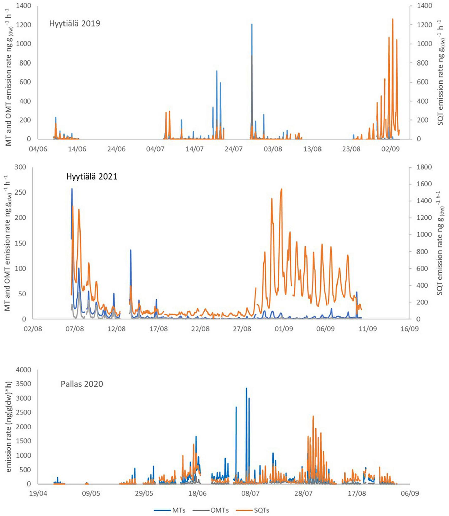
Monoterpene, oxygenated monoterpene and sesquiterpene emission rates in Hyytiälä and Pallas.
APPENDIX FIGURE 2
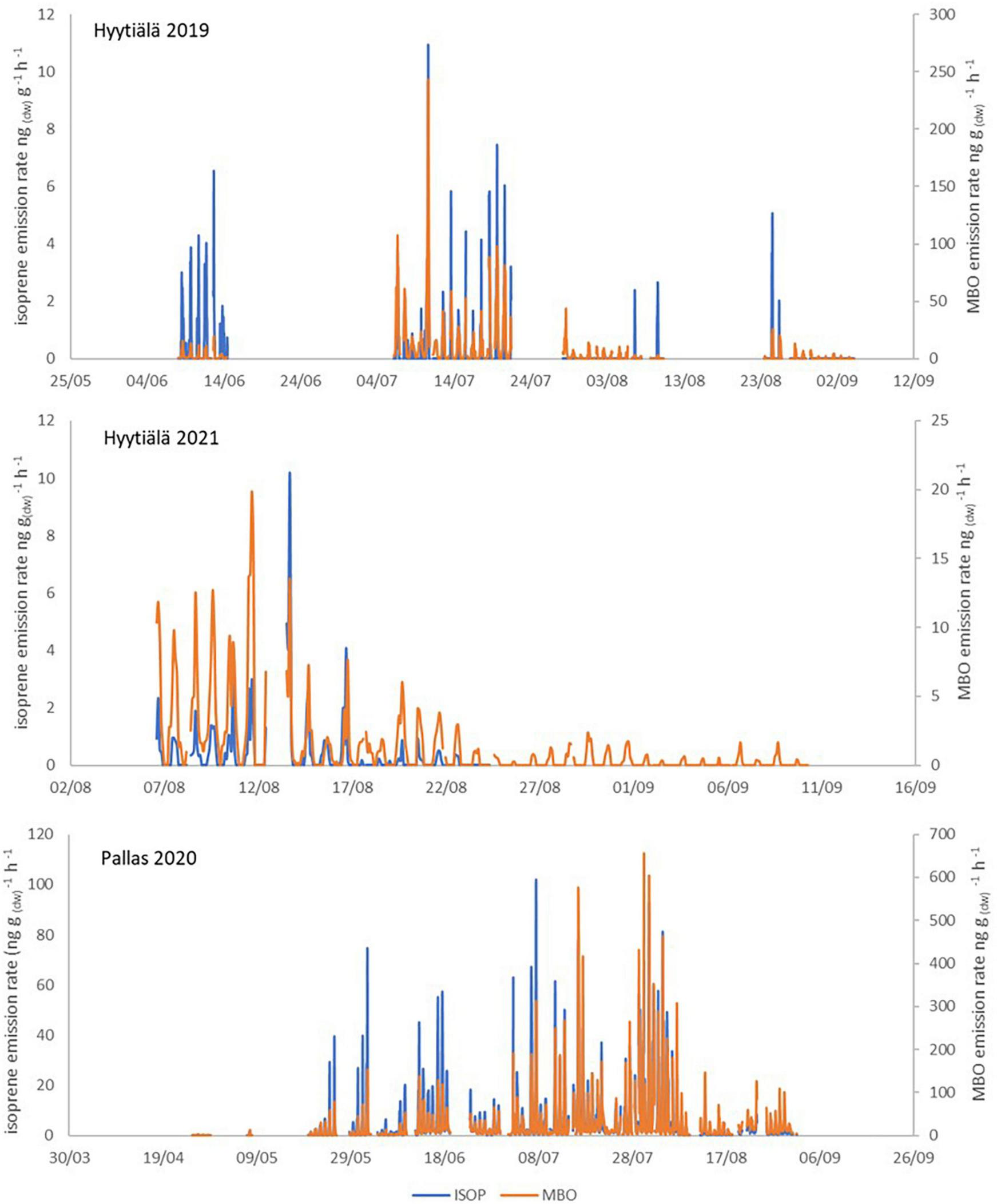
Isoprene and MBO emission rates in Hyytiälä and Pallas.
Summary
Keywords
biogenic volatile organic compound emissions, monoterpene, sesquiterpene, isoprene, Norway spruce emissions, SOA formation
Citation
Hakola H, Taipale D, Praplan A, Schallhart S, Thomas S, Tykkä T, Helin A, Bäck J and Hellén H (2023) Emissions of volatile organic compounds from Norway spruce and potential atmospheric impacts. Front. For. Glob. Change 6:1116414. doi: 10.3389/ffgc.2023.1116414
Received
05 December 2022
Accepted
28 February 2023
Published
23 March 2023
Volume
6 - 2023
Edited by
Yongjie Li, University of Macau, Macao SAR, China
Reviewed by
Steffen M. Noe, Estonian University of Life Sciences, Estonia; Pallavi Saxena, University of Delhi, India
Updates
Copyright
© 2023 Hakola, Taipale, Praplan, Schallhart, Thomas, Tykkä, Helin, Bäck and Hellén.
This is an open-access article distributed under the terms of the Creative Commons Attribution License (CC BY). The use, distribution or reproduction in other forums is permitted, provided the original author(s) and the copyright owner(s) are credited and that the original publication in this journal is cited, in accordance with accepted academic practice. No use, distribution or reproduction is permitted which does not comply with these terms.
*Correspondence: Heidi Hellén, heidi.hellen@fmi.fi
This article was submitted to Forests and Global Change Forests and the Atmosphere, a section of the journal Frontiers in Forests and Global Change
Disclaimer
All claims expressed in this article are solely those of the authors and do not necessarily represent those of their affiliated organizations, or those of the publisher, the editors and the reviewers. Any product that may be evaluated in this article or claim that may be made by its manufacturer is not guaranteed or endorsed by the publisher.