Abstract
Vegetation cover degradation is often a complex phenomenon, exhibiting strong correlation with climatic variation and anthropogenic actions. Conservation of biodiversity is important because millions of people are directly and indirectly dependent on vegetation (forest and crop) and its associated secondary products. United Nations Sustainable Development Goals (SDGs) propose to quantify the proportion of vegetation as a proportion of total land area of all countries. Satellite images form as one of the main sources of accurate information to capture the fine seasonal changes so that long-term vegetation degradation can be assessed accurately. In the present study, Multi-Sensor, Multi-Temporal and Multi-Scale (MMM) approach was used to estimate vulnerability of vegetation degradation. Open source Cloud computing system Google Earth Engine (GEE) was used to systematically monitor vegetation degradation and evaluate the potential of multiple satellite data with variable spatial resolutions. Hotspots were demarcated using machine learning techniques to identify the greening and the browning effect of vegetation using coarse resolution Normalized Difference Vegetation Index (NDVI) of MODIS. Rainfall datasets of Climate Hazards Group InfraRed Precipitation with Station data (CHIRPS) for the period 2000–2022 were also used to find rainfall anomaly in the region. Furthermore, hotspot areas were identified using high-resolution datasets in major vegetation degradation areas based on long-term vegetation and rainfall analysis to understand and verify the cause of change whether anthropogenic or climatic in nature. This study is important for several State/Central Government user departments, Universities, and NGOs to lay out managerial plans for the protection of vegetation/forests in India.
1 Introduction
Land is referred as an entity with zero consumption rate (Thepade and Chaudhari, 2021). Therefore, it is one of the most important resources to maintain the functioning of the socioeconomic system perfectly (Xie et al., 2022). Degradation of land is based on the continuous or long-term loss of natural resources. World’s 40% of land area is currently degraded and is increasing over time and directly threatening (Shao et al., 2024). Among all landscapes, forests are critical strongholds for environmental services and can help for ecological restoration (Fa et al., 2020; Sharma et al., 2022) apart from forest monitoring, natural resources such as agriculture monitoring is also important for understanding the consequence of a mismatch between land suitability and land use (Kılıç et al., 2024). According to the Forest Resource Assessment by Food and Agriculture Organization (FAO), 4 billion hectares of global land come under forest, half of which is found in the tropics and subtropics (Forneri et al., 2006; Singh et al., 2022; Nabuurs et al., 2023). Among all land uses, quantifying forest extent and change in forest is most important not only because forest protects climatic condition but also it supplies most essential flow of ecosystem services, such as fiber, energy, supports biodiversity, carbon storage, flux, and water (Coulston et al., 2014; Ferreira et al., 2023). Due to massive importance of forests, United Nations Framework Convention on Climate Change (UNFCCC) has shown significant interest on the protection of forest patches; the convention outlined that forest degradation contributes to total global carbon emission to a large extent, leading to global warming, and therefore, forest degradation needs immediate protection (Gao et al., 2020; Liang and Gamarra, 2020).
Tropical forests have always been critically acclaimed for rainfall generation because forests in these areas produce rainfall twice more than in any other latitude (Doughty et al., 2023); therefore, forest degradation in these regions can cause a reverse convective cloud cover and disturb the global rainfall circle (Watson et al., 2018; King et al., 2024). Tropical forest is niche of several species (Noulèkoun et al., 2024); therefore, deforestation and degradation of forest can lead to the extinction of biological diversity by habitat destruction and isolation of formerly contiguous forest and significant physical and biological consequences at the fringe or boundary zone between forest and deforested areas (Gascon et al. 2000; Rani et al., 2024). In the past, tropical deforestation globally reported approximately 1.1–2.2 PgC/year release (Gullison et al. 2007; Sasaki and Putz, 2009, Pujar et al., 2024) due to continuous increase in threats and pressure on forest resources; therefore, it is believed that demand for quantitative measurement, timely and accurately, can help in sustainable management of forests.
Earlier studies have often suggested that forest degradation is one of the major reasons for the discrepancy of forest cover maps (Sexton et al., 2015; Qin et al., 2024). To overcome this draw back, UNFCCC has defined forest as an area of more than 0.5–1.0 ha with tree crowning covering 10–30% (UNFCCC, 2002; Romijn et al., 2013; Asante et al., 2017). Furthermore, the convention has recognized forest habitats as important factors influencing the decline in forest-dependent fauna and flora (Rurangwa et al., 2021); therefore, it is important to understand forest degradation for forest restoration work (Roy et al., 2013; Jashimuddin et al., 2024). Southeast Asian countries have highest rate of tropical deforestation globally (Miettinen et al., 2011; Chen et al., 2023; Stan et al., 2024). In this region, food insecurity and poverty are the main concern enduring undue pressure on agricultural and forested land, and therefore, reconciliation of these lands is the main priority (Carrasco et al., 2016; Gonzalez-Redin et al., 2024). India is one of the mega-biodiversity nations lying in junction between three major biogeographic realms, namely, the Indo-Malayan, the Eurasian, and the Afro-tropical (Reddy et al., 2015). According to Forest Survey of India (FSI) reports, the country’s forest covers 7, 13,789 km2 (Forest Survey of India, 2021), which represents 21% of the total geographical area of the country. Although change in forest cover is highly debatable due to seasonal inference in countries such as India, Pasha and Dadhwal, 2024 claimed that forest cover is declining at the rate of 2.43 ha across the country.
In recent decades, remote sensing has gained its popularity due to its unique capability for providing imageries of the Earth’s surface in such a way that it allows easy identification of features, location, and characteristics in accordance to different time span (Singh et al., 2022; Chauhan et al., 2024). Remote sensing technologies use spectral properties to reveal information regarding the health of the canopies (Houborg et al., 2015; Wen et al., 2024). The vegetation dynamics of any land mass have always been treated as a significant indicator that can be used to quantitatively detect ecosystem processes at different scales by remote sensing experts (Sur et al., 2018). Absorption of leaf signatures is prominent due to leaf pigmentation (such as chlorophylls, carotenoids, and xanthophylls) in the visible spectral region (400–700 nm), with moderate absorptions by water in the shortwave-infrared (SWIR, 1300–2,100 nm) and only slight absorption by leaves in the near-infrared (NIR, 700–1,300 nm) region (Huete, 2012; Santana et al., 2024). To add further, in recent years, the increased availability of computing power through openly available cloud platforms (e.g., Google Earth Engine) and readily accessible machine learning algorithms from open source software tools (e.g., Python Scikit-learn) has enabled the processing of large volumes of satellite imagery over increasingly large geographical areas with reduced complexity and time (Gorelick et al., 2017; Sur et al., 2021; Verma et al., 2023; Singh et al., 2024). Therefore, this study is designed to make a spatial framework in GEE to compute forest degradation using a special Multi-Sensor, Multi-Temporal and Multi-Scale (MMM) approach. This approach is unique of its own because it will help to assess vegetation degradation over any selected period. This particular study is based on the temporal window 2000–2022 in a single frame capturing three distinct seasonal variations (summer, monsoon, and winter) using machine learning techniques for entire India. Furthermore, it demonstrates the distinctive utility of satellite images in GEE platform to identify the hotspots and evaluate the causes of vegetation degradation and take sustainable combating measures.
2 Study area
The study area (Figure 1) is focused on Indian landmass comprising of 28 states and 8 union territories. Since 1990, after economic liberalization of India, socio-economic development lead to considerable stress on the natural ecosystem (Visser, 2017), which needs immediate sustainable management strategies. Therefore, the study concentrates on vegetation including 14 major forest types of India based on multi-season satellite images, biogeography, climate, and elevation. Wet evergreen and semi evergreen forests are mainly located in the high-rainfall areas of Western Ghats, Andaman and Nicobar Islands, and north eastern region. Central India is mainly dominated by dry and moist deciduous forests. Mangroves are found in the coastal region of West Bengal, Odisha, Andhra Pradesh, Tamil Nadu, Maharashtra, Goa, and Gujarat. Montane, sub-alpine, and sub-tropical pine forests are distributed in the high-altitude Himalayan and north-east regions (Chakraborty et al., 2018). India has a typical climatic condition, often affected by heat waves, cold waves, fog, snowfall, floods and droughts, monsoon depressions, and cyclones (Dash et al., 2007). Combined action of physical factors and socio-economic factors makes Indian landmass more vulnerable and fragile.
Figure 1

Study area.
3 Methodology
The overall methodology adopted for the study is shown in Figure 2. Google Earth Engine (GEE) is an open source platform for geospatial data analysis. Its interface used in this study uses Java script and Python for data processing. The entire methodology can be divided into four broad structural domains: (i) selection of database for analysis, (ii) technical algorithm for understanding greening and browning, (iii) technical algorithm for understanding anomaly leading to wet and dry regions, (iv) visualization of degraded vegetation in high resolution.
Figure 2

Schematic diagram of the methodology.
3.1 Selection of database for analysis
3.1.1 Vegetation index datasets
The vegetation index product MOD13Q1 (V6.1) (Didan et al., 2015) is provided by Terra Moderate Resolution Imaging Spectroradiometer (MODIS). This study uses this product from 2000 to 2022 for analysis. It consists of two layers (a) Normalized Difference Vegetation Index (NDVI) and (b) Enhanced Vegetation Index (EVI) per pixel basis. The EVI layer minimizes canopy background variations and maintains sensitivity over dense vegetation conditions. The EVI also uses the blue band to remove residual atmosphere contamination caused by smoke and sub-pixel thin cloud. The EVI products are computed from atmospherically corrected bi-directional surface reflectance that has been masked for water, clouds, heavy aerosols, and cloud shadows. This product provides dataset of 250-m spatial resolution.
3.1.2 Rainfall datasets
Dataset from Climate Hazards Group Infra Red Precipitation with Station data (CHIRPS) is a quasi-global rainfall dataset (Funk et al., 2012). The CHIRPS dataset incorporates 0.05° resolution satellite imagery with in-situ station data to create gridded rainfall time series for trend analysis and seasonal monitoring of rainfall. In this study, monsoon datasets for the period 2000–2022 were utilized to compute the anomaly of the rainfall distribution.
3.1.3 Landsat datasets
Landsat is a joint program of the USGS and NASA, and since 1972 it has been observing the Earth continuously. The Landsat satellites image the entire surface of the Earth at a 30-m resolution approximately once every 2 weeks, including multispectral and thermal data. Three bands (Red, Green, and Blue) were used for monitoring vegetation degradation between 2000 and 2022.
3.1.4 Technical algorithm for understanding greening and browning
Theil–Sen slope and Mann–Kendall test were used to analyze long term (2000–2022) vegetation trend in a time-series of each pixel (Fensholt et al., 2012). Theil–Sen slope algorithm was preferred because of its efficiency to handle huge discrete dataset, and on the other hand, Mann–Kendall test was used along with Theil–Sen slope due to its advantage of not requiring samples to confirm a specific distribution and is free from the effect of outliers’ interference (Feng et al., 2023). Therefore, this study uses Theil– Sen slope and Mann–Kendall test to estimate the greening and browning trend of the time-series over the forest cover.
3.1.5 Technical algorithm for understanding rainfall anomaly
The impact of rainfall variability on vegetation in Indian landscape was characterized based on the analysis of time-series anomalies. The response of vegetation to moisture availability was analyzed, especially in dry, normal, and wet years. The spatiotemporal variability in rainfall anomalies was produced using the annual mean rainfall from 2000 to 2022. Equation (1) is the standard anomaly equation which is generally used in statistics to estimate the Z-score (Atkinson et al., 2011). Since the study covers a vast region, rainfall quantity is different in dry and wet regions. Thus, we have to standardize rainfall in order to compare the relative variability across the country.
where RA (i, x, y) represents the annual standardized rainfall anomaly in the ith year at the pixel location (x, y) and rainfall (i, x, y) represents the annual rainfall of ith year being processed. Mean [rainfall 2000–2022 (i, x, y)] represents the long-term mean annual rainfall from 2000 to 2022. STD [rainfall 2000–2022 (i, x, y)] represents the standard deviation of annual rainfall from 2000 to 2022.
3.1.6 Visualization in high resolution
Places with high browning trend in all three seasons and high rainfall anomaly were further observed in high-resolution datasets to infer the actual cause of the vegetation degradation.
4 Results and analysis
The main approach of this study was based on Multi-Sensor, Multi-Temporal and Multi-Scale (MMM) approach in an automotive way using cloud computing system Google Earth Engine (GEE) to identify vegetation degradation easily. The distinct patterns in three seasons (summer, monsoon, and winter) clearly demonstrated the role of climate variation in the region. In Figure 3, monsoon has the most greening effect with respect to the other two seasons, summer shows maximum browning effect, and winter shows moderate browning effect in the region. It is carefully observed that mostly degraded vegetation boundaries are clearly found in extreme eastern part of the country in the Seven Sisters states, Punjab, and Haryana foot hill region and a small portion of Jharkhand and Odisha.
Figure 3

Greening and browning trend of NDVI for the time span 2000–2022.
The bar graph in Figure 4 and Table 1 shows the browning and greening effect of summer season in India. The browning effect is most prominent in Madhya Pradesh due to the presence of large forest area in the state, which is highly affected in summer. Approximately 131271.577 km2 is under browning in this region, whereas 177416.1116 km2 remains green even in summer. Among Union territories, the most affected region is Delhi during summer, wherein approximately 516.049 km2 is affected by browning.
Figure 4

Bar Graph showing greening and browning trend of vegetation for the time span 2000–2022 for 29 states of India and 6 Union territories in summer season.
Table 1
| Summer | Monsoon | Winter | |||||
|---|---|---|---|---|---|---|---|
| Sl no | State | Browning sq. km | Greening sq. km | Browning sq. km | Greening sq. km | Browning sq. km | Greening sq. km |
| 1 | Jammu & Kashmir | 66013.486 | 176876.5686 | 35929.861 | 206920.8158 | 56466.583 | 186193.9775 |
| 2 | Punjab | 22508.028 | 28565.8836 | 3550.737 | 47522.15783 | 7344.427 | 43768.66949 |
| 3 | Himachal Pradesh | 15462.6 | 20567.9476 | 8130.016 | 27896.22283 | 7076.757 | 28971.59049 |
| 4 | Uttaranchal | 21678.594 | 32656.7856 | 9378.011 | 44956.74183 | 10298.69 | 44044.87849 |
| 5 | Chandigarh* | 60929.281 | 75186.5716 | 25315.498 | 110804.4798 | 23379.589 | 112688.2965 |
| 6 | Rajasthan | 55987.347 | 286978.2266 | 23243.451 | 319787.2778 | 32301.089 | 310662.8115 |
| 7 | Haryana | 9739.95 | 35029.8156 | 4131.619 | 40634.58383 | 6603.677 | 38203.26349 |
| 8 | Delhi* | 516.049 | 1650.2746 | 562.095 | 1600.501829 | 579.53 | 1626.116486 |
| 9 | Arunachal Pradesh | 43534.45 | 39209.3466 | 26164.26 | 56573.16683 | 19591.843 | 63103.60949 |
| 10 | Nagaland | 9994.642 | 7261.1916 | 7314.766 | 9936.067829 | 2620.257 | 14668.06549 |
| 11 | Madhya Pradesh | 131271.577 | 177416.1116 | 68656.221 | 240045.0338 | 17012.002 | 291667.6935 |
| 12 | Meghalaya | 12200.123 | 10902.8306 | 11348.144 | 11748.95783 | 4386.73 | 18744.75049 |
| 13 | Manipur | 10165.275 | 12797.5396 | 8151.392 | 14806.29583 | 5560.574 | 17423.17349 |
| 14 | Assam | 33869.441 | 45240.3386 | 29608.607 | 49495.31483 | 20016.481 | 59065.13449 |
| 15 | Uttar Pradesh | 106645.535 | 134672.9376 | 26652.777 | 214686.8948 | 29904.965 | 211442.9805 |
| 16 | Bihar | 35123.207 | 59593.1386 | 11348.569 | 83371.00283 | 9616.885 | 85129.45349 |
| 17 | Mizoram | 10409.014 | 11346.5716 | 8554.759 | 13196.21583 | 7330.816 | 14443.01349 |
| 18 | Tripura | 5570.793 | 5528.8246 | 4126.637 | 6968.527829 | 3171.655 | 7956.244486 |
| 19 | Jharkhand | 34847.713 | 45686.6136 | 9948.728 | 70589.14483 | 10201.733 | 70346.60549 |
| 20 | West Bengal | 17289.127 | 70204.7786 | 16371.478 | 71114.03483 | 16258.81 | 71207.99049 |
| 21 | Gujarat | 86634.994 | 95392.2306 | 29945.085 | 152090.6838 | 17100.133 | 164865.9235 |
| 22 | Daman & Diu* | 48.34 | 707.7386 | 47.989 | 703.6768286 | 13.586 | 782.6464857 |
| 23 | Dadra & Nagar Haveli | 341.612 | 814.8826 | 114.657 | 1037.602829 | 70.889 | 1125.399486 |
| 24 | Maharashtra | 83469.906 | 224397.7726 | 41188.338 | 266684.0588 | 24637.307 | 283181.5905 |
| 25 | Pondicherry* | 168.227 | 992.7776 | 125.209 | 1032.237829 | 190.869 | 1009.474486 |
| 26 | Goa | 1803.121 | 2481.2346 | 1217.836 | 3062.502829 | 447.244 | 3873.245486 |
| 27 | Tamil Nadu | 31548.307 | 98796.6416 | 32504.04 | 97837.53683 | 22773.762 | 107465.5355 |
| 28 | Kerala | 16631.058 | 22713.1226 | 17556.248 | 21780.94083 | 13975.62 | 25381.80349 |
| 29 | Lakshadweep* | 17.148 | 671.4906 | 13.357 | 671.0888286 | 15.678 | 712.8414857 |
| 30 | A & N Islands* | 3016.06 | 4160.0956 | 2459.623 | 4711.066829 | 1900.724 | 5287.202486 |
| 31 | Sikkim | 2803.369 | 4991.1926 | 1675.059 | 6115.818829 | 1333.003 | 6493.378486 |
| 32 | Odisha | 38156.318 | 117461.0556 | 21436.843 | 134180.1768 | 19145.658 | 136486.5045 |
| 33 | Andhra Pradesh | 48212.1 | 112289.9836 | 44853.119 | 115655.9258 | 30182.601 | 130308.8615 |
| 34 | Karnataka | 44213.755 | 147715.4386 | 34269.637 | 157664.8398 | 35351.268 | 156560.6435 |
| 35 | Telengana | 37537.912 | 77946.5866 | 18037.988 | 97448.74883 | 20946.948 | 94561.24749 |
| TGA | 3,287,263 | 3,287,263 | 3,287,263 | ||||
Long-term dynamics of vegetation (greening and browning) for 29 states of India and 6 Union territories.
*Union Territory.
Maximum rainfall in India is received in monsoon season during July and mid-November. The bar graph in Figure 5 and Table 1 shows the browning and greening effects of monsoon season in India. The greening effect is most prominent in monsoon season due to the availability of water in the country from rainfall. Rajasthan, the driest state of India, also shows profound greening effect on monsoon (319787.27 km2) because this is the only season in which vegetation and crop growth in Rajasthan is abundantly observed in the area. Apart from Punjab and Haryana, the two most agriculturally dominating states show a high concentration of greening area during Monsoon. Punjab state shows 47522.15 km2 under greening and 3550.737 km2 as browning, whereas Haryana state shows 40634.58 km2 under greening and 4131.61 km2 under browning.
Figure 5
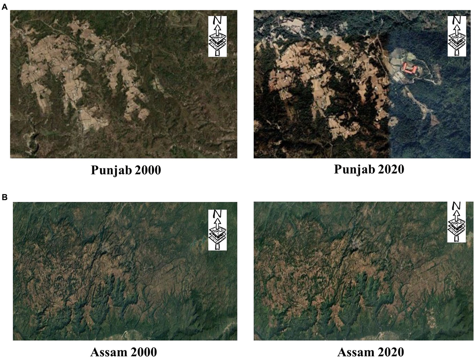
Examples of Vegetation Degradation Hotspots.
Winter season in India is very crucial because in most regions, it offer a chance for dual cropping, but on the other hand, deciduous forest in India suffer from browning effect and leaf shedding during this period, except for rain forests. Considering this reason, our analysis also brings out the fact that northern part of Himalayas remains green even in winter, while the degradation in vegetation is clearly observed as we come down to lower Himalayas or southern part of the region. The dynamics of vegetation degradation is exactly opposite to that of summers. The greening of vegetation is maximum in Madhya Pradesh during winter, wherein greening and browning is 291667.69 km2 and 17,012 km2, respectively. Apart from Madhya Pradesh, greening is also observed more in states of Gujarat and Maharashtra.
From the bar graphs shown in Figures 4–6, it is clear that almost all the states are undergoing browning effect in India. Alarming proportions are observed in Jammu and Kashmir, Odisha, and Andhra Pradesh, apart from the North-Eastern states such as Assam, Nagaland, Mizoram, Tripura, Manipur, Arunachal Pradesh, and Meghalaya. The proportion of forest cover in North Eastern India and Jammu and Kashmir is high because less agricultural land is available and the terrain is composed of hard and rocky mountains. Therefore, these regions are very vulnerable and needs proper management of plans over time by central and local government bodies.
Figure 6
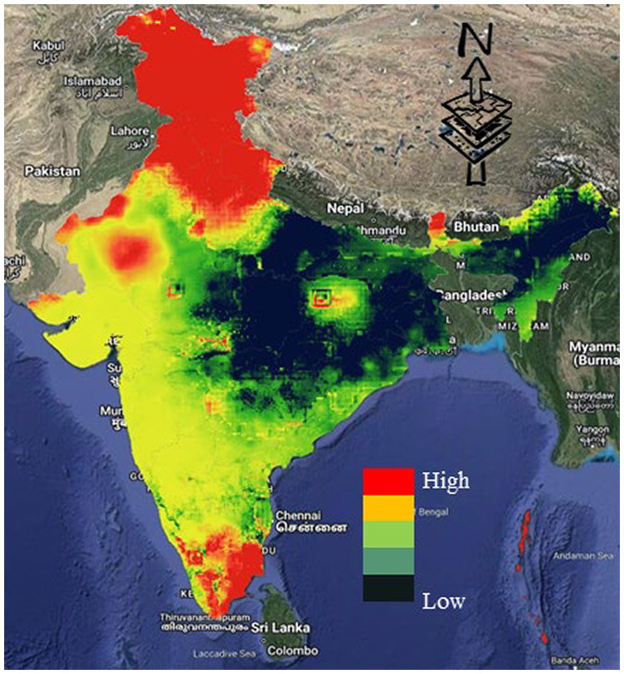
Rainfall Anomaly from 2000-2020.
Since rainfall in India is predominantly dependent on the monsoon, the rainfall datasets of monsoon months from July to October were considered. According to Figure 5, it is clear that anomaly of rainfall is high in the regions, which significantly shows red in color during 2000–2022, indicating them as dry zone, whereas on the other hand, the region which is almost black indicates that mostly the rainfall is constant over the selected years during monsoon season. Resultantly, the rainfall variation might affect the vegetation/forest cover in India because rainfall has significant effect on soil moisture and other climatic phenomena.
After the greening and browning analysis, the vegetation degradation hotspots were clearly visible; therefore, Natural Color Composite (RGB) was built using the Landsat archive datasets to clearly visualize the changes in forest cover in GEE. Two hot spot zones, namely, (a) Punjab and (b) Assam are shown as representatives of the entire study area. Two years (2000–2022) RGB datasets of Punjab clearly demonstrate the encroachment/anthropogenic pressure leading to the degradation of vegetation cover, and Assam forest patch has been cleared for agricultural purposes.
5 Conclusion
Remote sensing-based vegetation indices and rainfall datasets for 22 years were used to investigate the response of forest cover over Indian landmass. The research revealed a complex spatial pattern of diverse vegetation responses to seasonal variation, which is expressed through long-term trends. Indian vegetation condition showed resistance to dry spells and water scarcity despite abrupt rainfall trends. This means that the productivity of vegetation has been sustained even during dry conditions in different years. Nevertheless, it was found that rainfall impacted vegetation growth to some extent: negatively in summer years (2002) and positively in monsoon years. The research presented here used a new technique, named as MMM technique, using Multi-Sensor, Multi-Temporal and Multi-Scale datasets, which helped to compute in a single platform, for a unique visualization for the first time so as to manage sustainable vegetation cover from further degradation. It is recommended to set up a network of rainfall stations, runoff measurements, phenocams, and eddy covariance towers, to quantify the impacts of climate change and assess vegetation degradation vulnerability relative to future changes/developments across India. Such a network may also help to understand the exchange of carbon and water fluxes, water use efficiency, and the impact of drought at the microlevel.
Statements
Data availability statement
The original contributions presented in the study are included in the article/supplementary material, further inquiries can be directed to the corresponding author.
Author contributions
KS: Conceptualization, Data curation, Formal analysis, Funding acquisition, Investigation, Methodology, Project administration, Resources, Software, Supervision, Validation, Visualization, Writing – original draft, Writing – review & editing. VV: Data curation, Formal analysis, Funding acquisition, Methodology, Project administration, Resources, Software, Supervision, Validation, Visualization, Writing – review & editing, Writing – original draft. PP: Funding acquisition, Project administration, Resources, Supervision, Visualization, Writing – review & editing. GS: Funding acquisition, Project administration, Resources, Supervision, Visualization, Writing – review & editing. SC: Funding acquisition, Project administration, Resources, Supervision, Writing – review & editing. AN: Funding acquisition, Project administration, Resources, Supervision, Visualization, Writing – review & editing.
Funding
The author(s) declare that no financial support was received for the research, authorship, and/or publication of this article.
Conflict of interest
The authors declare that the research was conducted in the absence of any commercial or financial relationships that could be construed as a potential conflict of interest.
Publisher’s note
All claims expressed in this article are solely those of the authors and do not necessarily represent those of their affiliated organizations, or those of the publisher, the editors and the reviewers. Any product that may be evaluated in this article, or claim that may be made by its manufacturer, is not guaranteed or endorsed by the publisher.
References
1
Asante W. A. Dawoe E. Acheampong E. Bosu P. P. (2017). A new perspective on Forest definition and shade regimes for Redd+ interventions in Ghana’s cocoa landscape.
2
Atkinson P. M. Dash J. Jeganathan C. (2011). Amazon vegetation greenness as measured by satellite sensors over the last decade. Geophys. Res. Lett.38. doi: 10.1029/2011GL049118
3
Carrasco L. R. Papworth S. K. Reed J. Symes W. S. Ickowitz A. Clements T. et al . (2016). Five challenges to reconcile agricultural land use and forest ecosystem services in Southeast Asia. Conserv. Biol.30, 962–971. doi: 10.1111/cobi.12786
4
Chauhan M. Sur K. Chauhan P. Joshi H. Singh A. P. Borkar A. S. (2024). Lithological mapping of Nidar ophiolite complex, Ladakh using high-resolution data. Advances in Space Research.
5
Chakraborty A. Seshasai M. V. R. Reddy C. S. Dadhwal V. K. (2018). Persistent negative changes in seasonal greenness over different forest types of India using MODIS time series NDVI data (2001–2014). Ecol. Indic.85, 887–903. doi: 10.1016/j.ecolind.2017.11.032
6
Chen S. Woodcock C. Dong L. Tarrio K. Mohammadi D. Olofsson P. (2023). Review of drivers of forest degradation and deforestation in Southeast Asia. Remote Sens. App. Soc. Environ.33:101129. doi: 10.1016/j.rsase.2023.101129
7
Coulston J. W. Reams G. A. Wear D. N. Brewer C. K. (2014). An analysis of forest land use, forest land covers and changes at policy-relevant scales. Forestry87, 267–276. doi: 10.1093/forestry/cpt056
8
Dash S. K. Jenamani R. K. Kalsi S. R. Panda S. K. (2007). Some evidence of climate change in twentieth-century India. Clim. Chang.85, 299–321. doi: 10.1007/s10584-007-9305-9
9
Didan K. Munoz A. B. Solano R. Huete A. (2015). MODIS vegetation index user’s guide (MOD13 series)35, 2–33.
10
Doughty C. E. Keany J. M. Wiebe B. C. Rey-Sanchez C. Carter K. R. Middleby K. B. et al . (2023). Tropical forests are approaching critical temperature thresholds. Nature621, 105–111. doi: 10.1038/s41586-023-06391-z
11
Fa J. E. Watson J. E. Leiper I. Potapov P. Evans T. D. Burgess N. D. et al . (2020). Importance of indigenous peoples’ lands for the conservation of intact Forest landscapes. Front. Ecol. Environ.18, 135–140. doi: 10.1002/fee.2148
12
Feng X. Tian J. Wang Y. Wu J. Liu J. Ya Q. et al . (2023). Spatio-temporal variation and climatic driving factors of vegetation coverage in the Yellow River Basin from 2001 to 2020 based on kNDVI. Forests14:620. doi: 10.3390/f14030620
13
Fensholt R. Langanke T. Rasmussen K. Reenberg A. Prince S. D. Tucker C. et al . (2012). Greenness in semi-arid areas across the globe 1981–2007—an earth observing satellite based analysis of trends and drivers. Remote Sens. Environ.121, 144–158. doi: 10.1016/j.rse.2012.01.017
14
Ferreira V. Albariño R. Larrañaga A. LeRoy C. J. Masese F. O. Moretti M. S. (2023). Ecosystem services provided by small streams: an overview. Hydrobiologia850, 2501–2535. doi: 10.1007/s10750-022-05095-1
15
Forest Survey of India (2021). India state of Forest report 2009. Dehradun: Forest Survey of India.
16
Forneri C. Blaser J. Jotzo F. Robledo C. (2006). Keeping the forest for the climate's sake: avoiding deforestation in developing countries under the UNFCCC. Clim. Pol.6, 275–294. doi: 10.1080/14693062.2006.9685602
17
Funk C. Michaelsen J. Marshall M. T. (2012). Mapping recent decadal climate variations in precipitation and temperature across eastern Africa. WardlowBrian D.AndersonMartha C.VerdinJames P.. Remote sensing of drought: innovative monitoring approaches, 331, 331–355. CRC Press: Boca Raton, FL.
18
Gao Y. Skutsch M. Paneque-Gálvez J. Ghilardi A. (2020). Remote sensing of forest degradation: a review. Environ. Res. Lett.15:103001.
19
Gascon C. Williamson G. B. da Fonseca G. A. (2000). Receding forest edges and vanishing reserves. Science, 288, 1356–1358.
20
Gonzalez-Redin J. Gordon I. J. Polhill J. G. Dawson T. P. Hill R. (2024). Navigating sustainability: revealing the hidden forces in social–ecological systems. Sustain. For.16:1132. doi: 10.3390/su16031132
21
Gorelick N. Hancher M. Dixon M. Ilyushchenko S. Thau D. Moore R. (2017). Google earth engine: planetary-scale geospatial analysis for everyone. Remote Sens. Environ.202, 18–27. doi: 10.1016/j.rse.2017.06.031
22
Gullison R. E. Frumhoff P. C. Canadell J. G. Field C. B. Nepstad D. C. Hayhoe K. et al . (2007). Tropical forests and climate policy. Science, 316, 985–986.
23
Houborg R. Fisher J. B. Skidmore A. K. (2015). Advances in remote sensing of vegetation function and traits. Int. J. Appl. Earth Obs. Geoinf.43, 1–6. doi: 10.1016/j.jag.2015.06.001
24
Huete A. R. (2012). Vegetation indices, remote sensing and forest monitoring. Geogr. Compass6, 513–532. doi: 10.1111/j.1749-8198.2012.00507.x
25
Jashimuddin M. Hasan M. H. Baul T. K. Chakma N. Hossen S. Dutta S. et al . (2024). Principles of people-centric forest restoration projects in South-Eastern Bangladesh: implications for sustainability. Restor. Ecol.32:e14087. doi: 10.1111/rec.14087
26
Kılıç M. Gündoğan R. Guenal H. (2024). An illustration of a sustainable agricultural land suitability assessment system with a land degradation sensitivity. Environ. Dev. Sustain.26, 6085–6107. doi: 10.1007/s10668-023-02951-5
27
King J. A. Weber J. Lawrence P. Roe S. Swann A. L. Val Martin M. (2024). Global and regional hydrological impacts of global Forest expansion. EGUsphere2024, 1–27. doi: 10.5194/egusphere-2024-710
28
Liang J. Gamarra J. G. (2020). The importance of sharing global forest data in a world of crises. Sci. Data7:424. doi: 10.1038/s41597-020-00766-x
29
Miettinen J. Stibig H. J. Achard F. (2014). Remote sensing of forest degradation in Southeast Asia—Aiming for a regional view through 5–30 m satellite data. Glob. Ecol. Conserv.2, 24–36.
30
Nabuurs G. J. Mrabet R. Hatab A. A. Bustamante M. Clark H. Havlík P. et al . (2023). “Agriculture, forestry and other land uses (AFOLU)” in Climate change 2022: Mitigation of climate change (New York: Cambridge University Press), 747–860.
31
Noulèkoun F. Mensah S. Dimobe K. Birhane E. Kifle E. T. Naab J. et al . (2024). Both the selection and complementarity effects underpin the effect of structural diversity on aboveground biomass in tropical forests. Glob. Ecol. Biogeogr.33, 325–340. doi: 10.1111/geb.13800
32
Pasha S. V. Dadhwal V. K. (2024). National analysis on variations in estimates of forest cover dynamics over India (2001–2020) using multiple techniques and data sources. Spat. Inf. Res., 1–11. doi: 10.1007/s41324-024-00570-4
33
Pujar G. S. Taori A. Chakraborty A. Mitran T. (2024). “Sensing climate change through earth observations: perspectives at global and National Level” in Digital agriculture: A solution for sustainable food and nutritional security (Cham: Springer International Publishing), 225–280.
34
Qin Y. Xiao X. Tang H. Dubayah R. Doughty R. Liu D. et al . (2024). Annual maps of forest cover in the Brazilian Amazon from analyses of PALSAR and MODIS images. Earth Sys. Sci. Data16, 321–336. doi: 10.5194/essd-16-321-2024
35
Rani M. Panda D. Allen M. L. Pandey P. Singh S. K. Singh R. (2024). Assessment and prediction of human-elephant conflict hotspots in the human dominated area of Rajaji-Corbett landscape, Uttarakhand, India. J. Nat. Conserv.79:126601. doi: 10.1016/j.jnc.2024.126601
36
Reddy C. S. Jha C. S. Diwakar P. G. Dadhwal V. K. (2015). Nationwide classification of forest types of India using remote sensing and GIS. Environ. Monit. Assess.187, 1–30. doi: 10.1007/s10661-015-4990-8
37
Romijn E. Ainembabazi J. H. Wijaya A. Herold M. Angelsen A. Verchot L. et al . (2013). Exploring different forest definitions and their impact on developing REDD+ reference emission levels: a case study for Indonesia. Environ. Sci. Pol.33, 246–259. doi: 10.1016/j.envsci.2013.06.002
38
Roy P. S. Murthy M. S. R. Roy A. Kushwaha S. P. S. Singh S. Jha C. S. et al . (2013). Forest fragmentation in India. Curr. Sci., 774–780.
39
Rurangwa M. L. Aguirre-Gutiérrez J. Matthews T. J. Niyigaba P. Wayman J. P. Tobias J. A. et al . (2021). Effects of land-use change on avian taxonomic, functional and phylogenetic diversity in a tropical montane rainforest. Divers. Distrib.27, 1732–1746.a. doi: 10.1111/ddi.13364
40
Santana D. C. Theodoro G. D. F. Gava R. de Oliveira J. L. G. Teodoro L. P. R. de Oliveira I. C. et al . (2024). A new approach to identifying Sorghum hybrids using UAV imagery using multispectral signature and machine learning. Algorithms17:23. doi: 10.3390/a17010023
41
Sasaki N. Putz F. E. (2009). Critical need for new definitions of “forest” and “forest degradation” in global climate change agreements. Conserv. Lett.2, 226–232. doi: 10.1111/j.1755-263X.2009.00067.x
42
Sexton J. O. Noojipady P. Song X.-P. Feng M. Song D.-X. Kim D.-H. et al . (2015). Conservation policy and the measurement of forests. Nat. Clim. Chang.6, 192–196. doi: 10.1038/nclimate2816
43
Shao W. Zhang Z. Guan Q. Yan Y. Zhang J. (2024). Comprehensive assessment of land degradation in the arid and semiarid area based on the optimal land degradation index model. Catena234:107563. doi: 10.1016/j.catena.2023.107563
44
Sharma A. Tracy J. Panwar P. (2022). “Ecological restoration of degraded forests for achieving land degradation neutrality” in Land degradation neutrality: Achieving SDG 15 by Forest management. ed. PanwarP. (Singapore: Springer Nature), 191–204.
45
Singh M. Arshad A. Bijlwan A. Tamang M. Shahina N. N. Biswas A. et al . (2024). Mapping tree carbon density using sentinel 2A sensor on Google earth engine in Darjeeling Himalayas: implication for tree carbon management and climate change mitigation. Phy. Chem. Earth, Parts A/B/C134:103569. doi: 10.1016/j.pce.2024.103569
46
Singh M. Shahina N. N. Das S. Arshad A. Siril S. Barman D. et al . (2022). “Forest resources of the world: present status and future prospects” in Land Degradation Neutrality: Achieving SDG 15 by Forest Management. eds. PanwarP.ShuklaG.BhatJ. A.ChakravartyS. (Singapore: Springer), 1–23.
47
Singh S. Sur K. Verma V. K. Pateriya B. (2022). Quantitative assessment of channel planform dynamics across Satluj River in North India over 45 years: analysis using geospatial techniques. Water Conser. Sci. Eng.7, 453–464. doi: 10.1007/s41101-022-00154-z
48
Stan K. D. Sanchez-Azofeifa A. Hamann H. F. (2024). Widespread degradation and limited protection of forests in global tropical dry ecosystems. Biol. Conserv.289:110425. doi: 10.1016/j.biocon.2023.110425
49
Sur K. Dave R. Chauhan P. (2018). Spatio-temporal changes in NDVI and rainfall over Western Rajasthan and Gujarat region of India. J. Agrometeorol.20, 189–195. doi: 10.54386/jam.v20i3.541
50
Sur K. Verma V. K. Pateriya B. (2021). Surface water estimation at regional scale using hybrid techniques in GEE environment-a case study on Punjab state of India. Remote Sens. App.24:100625. doi: 10.1016/j.rsase.2021.100625
51
Thepade S. D. Chaudhari P. R. (2021). Land usage identification with fusion of thepade SBTC and sauvolathresholding features of aerial images using ensemble of machine learning algorithms. Appl. Artif. Intell.35, 154–170. doi: 10.1080/08839514.2020.1842627
52
UNFCCC (2002) Report of the conference of the parties on its seventh session, held at Marrakesh from 29 October to 10 November 2001 (FCCC/CP/2001/13/add.1, UNFCCC, Marrakesh, Morocco, 2001). Available at:http://unfccc.int/resource/docs/cop7/13a01.pdf
53
Verma V. K. Sur K. Prakash C. (2023). Ecotope-based diversity monitoring of wetland using infused machine learning technique. Water Conserv. Sci. Eng.8:38. doi: 10.1007/s41101-023-00212-0
54
Visser W. (Ed.) (2017). The world guide to sustainable Enterprise-volume 3: Europe. London: Routledge.
55
Watson J. E. Evans T. Venter O. Williams B. Tulloch A. Stewart C. et al . (2018). The exceptional value of intact forest ecosystems. Nat. Ecol. Evol.2, 599–610. doi: 10.1038/s41559-018-0490-x
56
Wen T. Liu J. Fu Y. Yue J. Li Y. Guo W. (2024). Development and evaluation of a new spectral index to detect Peanut southern blight disease using canopy hyperspectral reflectance. Horticulturae10:128. doi: 10.3390/horticulturae10020128
57
Xie W. Yu H. Li Y. Dai M. Long X. Li N. et al . (2022). Estimation of entity-level land use and its application in urban sectoral land use footprint: a bottom-up model with emerging geospatial data. J. Ind. Ecol.26, 309–322. doi: 10.1111/jiec.13191
Summary
Keywords
vegetation, land degradation, MMM approach, remote sensing, sustainability
Citation
Sur K, Verma VK, Panwar P, Shukla G, Chakravarty S and Nath AJ (2024) Monitoring vegetation degradation using remote sensing and machine learning over India – a multi-sensor, multi-temporal and multi-scale approach. Front. For. Glob. Change 7:1382557. doi: 10.3389/ffgc.2024.1382557
Received
05 February 2024
Accepted
15 May 2024
Published
06 June 2024
Volume
7 - 2024
Edited by
Kevin Boston, University of Arkansas at Monticello, United States
Reviewed by
Hayssam M. Ali, King Saud University, Saudi Arabia
Bhupendra Singh, VCSG Uttarakhand University, India
Updates
Copyright
© 2024 Sur, Verma, Panwar, Shukla, Chakravarty and Nath.
This is an open-access article distributed under the terms of the Creative Commons Attribution License (CC BY). The use, distribution or reproduction in other forums is permitted, provided the original author(s) and the copyright owner(s) are credited and that the original publication in this journal is cited, in accordance with accepted academic practice. No use, distribution or reproduction is permitted which does not comply with these terms.
*Correspondence: Koyel Sur, koyelsur3@gmail.com
Disclaimer
All claims expressed in this article are solely those of the authors and do not necessarily represent those of their affiliated organizations, or those of the publisher, the editors and the reviewers. Any product that may be evaluated in this article or claim that may be made by its manufacturer is not guaranteed or endorsed by the publisher.