Abstract
Accurate mapping of tree species is critical for forest management, carbon sequestration estimates and ecosystem assessment. Remote sensing provides an efficient approach using satellite image time series (SITS), but complex data poses challenges for classifiers and feature analysis. This study presents a deep learning-based classification method using Sentinel-1/2 SITS for mapping forest tree species and tree species biodiversity. Specifically, temporal data from unlabeled forest pixels were used for pretraining the model through self-supervised learning, followed by fine-tuning with species samples, enhancing model performance. Various configurations of temporal data were tested for classification, and their impact was evaluated. To address species maps accuracy overestimation caused by homogeneous pure-species stands, a pseudo-labeling approach was employed to incorporate mixed-species scenarios. Additionally, statistical and visualization methods were applied to SITS and model analysis. The results showed that longer time series tended to improve species identification and model confidence, with OA increasing from 0.496 (6–7 months) to 0.795 (1–12 months), macro-F1 from 0.384 to 0.779, and a significant improvement in predicted scores. As data from subsequent year was incorporated, accuracy growth slowed and stabilized, reaching OA of 0.847 and macro-F1 of 0.836, compared to 0.764 and 0.737 for the non-pretrained model. Certain vegetation indices, such as NDre and NDVIre, which are sensitive to physiological changes, highlight species differences during key phenological stages, especially between deciduous and evergreen species. This study demonstrates the potential of combining SITS with deep learning for species classification and provides a comprehensive analysis, contributing to ecological research and sustainable forest management.
1 Introduction
Forests are a key component of ecosystems, playing a crucial role in environmental sustainability and human wellbeing. Accurate mapping of forest tree species distribution and biodiversity is essential for forest management and conservation, ecosystem assessment, and the quantification of ecosystem carbon storage (Felton et al., 2020; Hermosilla et al., 2022; Wang and Gamon, 2019; Xiao et al., 2019). Tree species distribution information is vital for various research, such as assessing the impact of extreme weather events or climate change on forest ecosystems, and improving biomass estimation accuracy through tree species data (Fassnacht et al., 2014; Kumar et al., 2024; Lindner et al., 2010; Zhang et al., 2023). Forest biodiversity is closely tied to productivity and influenced by tree species composition, and biodiversity loss can significantly reduce forests carbon absorption capacity, affecting global carbon sequestration (Shirima et al., 2015). In many regions, tree species maps are typically derived from field surveys, the high costs of surveys often result in forest inventories being conducted only at multi-year intervals and species maps are not wall-to-wall. This does not meet the needs for mapping forest species over larger areas, and the accessibility and adequacy of existing data remain challenges (Blickensdörfer et al., 2024; White et al., 2016).
Remote sensing offers a promising and more cost-effective alternative to traditional field surveys (Kollert et al., 2021; Lechner et al., 2020). Earth observation satellites, such as Landsat and Sentinel, provide continuous images of the earth’s surface. These satellites can capture repeated images every few days and compose satellite image time series (SITS), which provide massive information about land cover (Miller et al., 2024). Moreover, these data can be processed and accessed for free through Google Earth Engine (GEE). Previous research has shown that the use of SITS yields excellent results, especially in vegetation studies, as multi-temporal images capture the phenological characteristics of plants more effectively (Foerster et al., 2012; Hemmerling et al., 2021). Phenological differences cause different tree species to be at various growth stages (e.g., greenness rise, leaf on, greenness fall, leaf off), leading to variations in appearance and physiological traits, resulting in distinct spectral reflectance and change patterns. Identifying distinct phenological characteristics and spectral-temporal changes among species has proven to be helpful for vegetation classification (Asner et al., 2008; Liu et al., 2023). Simply stacking multi-temporal images may lead to the omission of critical information due to algorithm limitations. Moreover, SITS often contain redundant features, increasing computational time and reducing classifier accuracy, a phenomenon known as the “curse of dimensionality”. The key challenge is how to mitigate the impact of high-dimensional data while identifying critical periods and optimal features (Camps-Valls et al., 2007; Hu et al., 2019; Löw et al., 2013). Common Machine Learning (ML) models such as Random Forest (RF), Support Vector Machine (SVM), have been widely explored for tree species classification (Fu et al., 2022; Hemmerling et al., 2021; Immitzer et al., 2019; Melnyk et al., 2023). However, these models process stacked temporal data independently, failing to capture the temporal dependencies inherent in the input (Ienco et al., 2017; Interdonato et al., 2019; Pelletier et al., 2019). Another problem is that traditional models rely heavily on input feature processing, struggling to leverage relationships between multi-temporal data and information redundancy. Consequently, many studies extracted key indicators based on feature selection algorithms or domain knowledge to enhance feature representation among species (Somers and Asner, 2014; Hu et al., 2019; You and Dong, 2020). Even so, feature engineering is time-consuming and challenging, and the resulting information is limited and highly dependent on the algorithms employed (Dou et al., 2021; Zhong et al., 2019).
Artificial intelligence (AI) has made significant advancements in the past few years, studies have shown that neural networks can identify and learn time dependencies in sequential data (Rußwurm and Körner, 2020; Zhong et al., 2019). In contrast to traditional ML, neural network-based deep learning (DL) automatically extract and learn features from vast amounts of data. Convolutional neural networks (CNNs) extract features in the short term through convolution, but may overlook long-term dependencies. Recurrent neural networks (RNNs) such as Long Short-Term Memory (LSTM), capture time dependencies by iteratively updating hidden state, which encodes information from previous time steps. However, this can increase computational complexity and noise, resulting in reduced efficiency (Rußwurm and Korner, 2017; Zhao et al., 2022). Transformer models based solely on the self-attention mechanism process long-term data without recursion, allowing each time step to compute correlations with others in parallel, thus enhancing training efficiency while mitigating noise accumulation and information loss (Vaswani et al., 2017). It has significantly impacted DL and has been effectively utilized in remote sensing research (Chen et al., 2022; Li et al., 2022). The advantages of Transformer in identifying key features and temporal dependencies makes it an excellent choice for tree species classification based on SITS. Given the scarcity of labeled data, a prevalent strategy involves combining pretrain and fine-tune. Pretraining a model on a large dataset allows it to learn general features and representations, followed by fine-tuning the model on a specific task dataset to adapt it for the intended purpose. This transfer of knowledge effectively enhances the model performance and generalization (Jing and Tian, 2021; Misra and Van Der Maaten, 2020). Although DL models demonstrate excellent performance, they are often considered as “black boxes” because of the hard interpretation of their decision-making processes. Explaining the feature learning pipeline can clarify the complex processes of information capture, supporting the reliability of results, and this explanatory process may also provide valuable insights for users (Lipton, 2018; Samek et al., 2017; Xu et al., 2021).
The Forest Inventory Data typically includes both pure and mixed species units, but many studies focus solely on pure stands, which may oversimplify scenarios like mixed stands and limit model generalization. Moreover, using the same source for validation may overestimate mapping accuracy (Blickensdörfer et al., 2024; Fassnacht et al., 2016). Adjusting the dataset to include more samples from diverse forest stands can address the limitations. Pseudo-labeling is a semi-supervised learning technique that generates labels for unlabeled samples through supervised training with labeled samples, enriching the dataset and improving model generalization (Blickensdörfer et al., 2024; Tan et al., 2015; Zhou, 2018). Combining DL with pseudo-labeling could achieve higher-quality dataset optimization, making it more representative of the study area forest.
The objective of this study is to employ a Transformer-based model to process SITS for tree species identification, while analyzing spectral-temporal data and interpreting the model. The model was pretrained on unlabeled forest pixels to enhance performance, and the dataset was optimized using Pseudo-labeling to include mixed-species scenes. Then the pretrained model was fine-tuned on the dataset, achieving precise forest tree species and tree species biodiversity mapping. Various methods based on statistic and visualization, were utilized to gain a comprehensive understanding of tree species classification using SITS and explore deep learning model. The original SITS data was analyzed from different perspectives, evaluating the contribution of spectral-temporal features, discussing the similarities and differences among tree species as well as the challenges of classification. Meanwhile, the impact of time series data composition on model performance was assessed and the model mechanism was analyzed.
2 Materials
2.1 Study area
The study area (approx. 35° 58′–37° 2′ E and 111° 45′–112° 32′ N) is located in the Shanxi Province, China. It includes the Huodong National Coal Mining Area and Taiyue Mountain National Forest Park, the largest forest reservation in Shanxi (Figure 1). The Taiyue Mountain and surrounding forests form an important nature reserve with a temperate continental climate, an average annual temperature of 9.2 °C, and 564 mm of precipitation. The study area covers a total of 7,715.17 km2, with elevations from 534 to 2,564 meters, and forests occupy 3,861.14 square kilometers, approximately 50% of the region, which belongs to the temperate northern forest zone. The main dominant tree species include: Larix principis-rupprechtii (LP), Pinus tabuliformis (PT), Pinus bungeana (PB), Platycladus orientalis (PO), Quercus wutaishanica (QW), Betula spp. (BA), Populus spp. (PS).
FIGURE 1

Study area and reference data. (A) The location of the study area in Shanxi Province, China. (B) The elevation information of study area. (C) The distribution of tree species reference data (Background: Sentinel-2 image from July 2023, bands R: 4, G: 3, B: 2; World Hillshade from ArcGIS Pro, Esri). Huodong: The Huodong National Coal Mining Area. Tree species: Larix principis-rupprechtii (LP), Pinus tabuliformis (PT), Pinus bungeana (PB), Platycladus orientalis (PO), Quercus wutaishanica (QW), Betula spp. (BA), Populus spp. (PS).
2.2 Remote sensing data
Based on the GEE platform, we used Sentinel-1 Ground Range Detected (GRD) backscatter products and Sentinel-2 MultiSpectral Instrument (MSI) Level-2A products from 2022 to 2023, including cloud removal, monthly median value extraction, and resampling to a spatial resolution of 10 meters, visit https://developers.google.com/earth-engine/datasets/catalog/sentinel for more details. We calculated commonly used vegetation indices and additional indices recognized in prior researches as valuable for vegetation remote sensing with Sentinel (Frampton et al., 2013; Li et al., 2014; Ngo et al., 2023; Schulz et al., 2024). Combined indices with the original bands, 33 variables include: B2-B8, B8A, B11-12, VV, VH, NDVI, GNDVI, LSWI, EVI, NDVIre1-3, NDre1-2, Clre, PSRI, MSAVI, MSRre, MTCI, CCCI, S2REP, RVI, VVVHR, NDIVV. Full names and formulas can be found in Supplementary Table S1. Temporal profiles of these indices for different tree species are provided in Supplementary Figures S1, S2, the plots highlight species-specific spectral, phenological, and structural differences, such as distinct temporal patterns between deciduous and evergreen trees, and backscatter contrasts between coniferous and broadleaf trees (Supplementary Figure S3).
The European Space Agency (ESA) WorldCover 10 m v200 product was used in this study to extract forest areas mask.
2.3 Ground reference dataset
As reference, we used the Forest Inventory data provided by Taiyue Mountain forest administration. The data was collected around 2020 and 2021 through field surveys and high-resolution images, recording forest resource attributes such as dominant and secondary species, stand age and area in polygons. We selected seven main tree species in the study area as target classes, categorizing other species as “Others” (mostly broadleaf) for the final tree species mapping (Figure 1). Reference points was randomly generated within each polygon, imposing constraints of over 20 meters between points and 30 meters from plot edges, and the number of points was based on plot area, resulting in a reference dataset. To address the simplification of mixed forest scenarios and accuracy overestimation resulting from the use of only pure-species samples, we also selected mixed-species plots to create pseudo-labeling samples, combining them with pure samples for DL model training and evaluation. The specific methods are detailed in section 3.1. We employed stratified sampling to select 60% of the samples from each species as an independent testing dataset to prevent data leakage (Table 1). The remaining 40% of samples were used for training and validation with five-fold cross-validation, each fold involved using one subset for validation. This process ensured validation on entirely different samples, aiming to thoroughly evaluate model performance, ensure generalization ability, and adjust model hyperparameters.
TABLE 1
| Short | Species | Type | Samples (pure: pseudo-labeled) | Training and validation | Testing |
| LP | Larix principis-rupprechtii | Deciduous | 8,924 (7,754:1,170) | 3,569 | 5,355 |
| PT | Pinus tabuliformis | Evergreen | 18,155 (11,936:6,219) | 7,262 | 10,893 |
| PB | Pinus bungeana | Evergreen | 4,666 (4,170:496) | 1,866 | 2,800 |
| PO | Platycladus orientalis | Evergreen | 8,532 (6,856:1,676) | 3,412 | 5,120 |
| QW | Quercus wutaishanica | Deciduous | 13,802 (8,710:5,092) | 5,520 | 8,282 |
| BA | Betula spp. | Deciduous | 8,053 (6,898:1,155) | 3,221 | 4,832 |
| PS | Populus spp. | Deciduous | 1,494 (1,322:172) | 597 | 897 |
| OT | Others | – | 2242 | 896 | 1,346 |
| Total | 65,868 | 26,343 | 39,525 |
The dataset for tree species mapping.
The tree species abbreviations, types, sample quantities (including pure units and pseudo-labeled samples); the number of samples used for training and validation in 5-fold cross-validation and for independent testing.
Additionally, forest mask was used to generate unlabeled pretraining forest samples by creating grid points at 100 m intervals (10 rows/columns for images), resulting in over 380,000 unlabeled samples.
3 Methods
3.1 Tree species dataset optimization
Forest inventory data consists of polygonal plots documenting the dominant and secondary tree species. Previous studies commonly used samples from pure units for model training and accuracy assessment (Immitzer et al., 2019; Yang et al., 2024), which may reduce dataset representativeness, lead to lower model performance in identifying mixed-species areas and overestimate mapping accuracy (Blickensdörfer et al., 2024). It’s easier to distinguish between evergreen and deciduous species due to their greater phenological feature differences. To ensure credibility for the pseudo samples added to the dataset, only mixed units of evergreen and deciduous species were used. Specifically, pure units of target tree species were selected firstly to generate pure samples, then evergreen-deciduous mixed units among the seven target tree species were selected to generate unlabeled samples. The process for generating pseudo-labels for unlabeled samples based on deep learning classification model are as Figure 2. First, the pretrained model was fine-tuned using labeled samples from pure units of two species (one evergreen and one deciduous), to obtain a binary classification model. Next, the unlabeled samples of mixed units were input into the binary classification model, which outputs predicted scores ranging from 0 to 1 for each sample. The class with the highest score was assigned as the pseudo-label, and samples with highest scores above 0.9 were added to the final dataset.
FIGURE 2
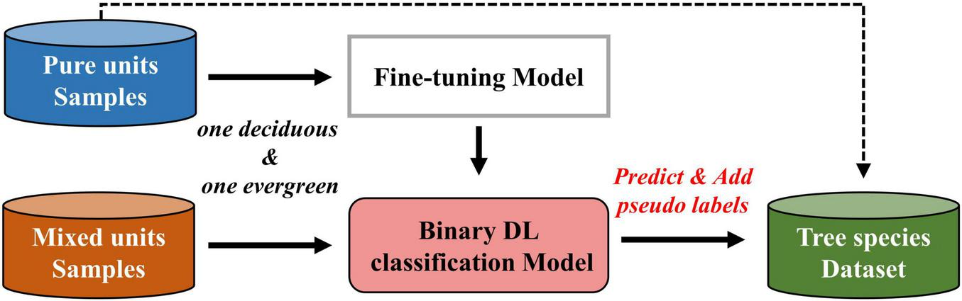
Optimizing the dataset through pseudo-labeled sample generation.
3.2 Classification model based on transformer
3.2.1 Transformer
The core of Transformer is the self-attention mechanism, which captures internal relationships between elements at any position in a sequence, excelling at handling long-term dependencies and capturing relevant information (Rußwurm and Körner, 2020). The complexity and temporal correlation of SITS data make Transformers an ideal choice for tree species classification tasks. The original pixels time series data X = {x1,x2,…,xn} is input, n representing the month. The data embedding process uses a linear dense layer to project the original time series observation data into a high-dimensional representation Linear(X), then the sine and cosine functions of different frequencies are used to generate “positional encodings”, which have the same dimension as the embeddings and are added to them (Vaswani et al., 2017):
Where n is the time position, i is the dimension index, and dmodel is the embedding dimension. The embedding dimension in this study is dmodel = 512.
The Em(X) is projected onto three matrices Q, K, V by stacking multiple query vectors (q), key vectors (k), and value vectors (v) using corresponding weight matrices WQ, WK, WV, these matrices are updated during the model training. Then, the scaled dot-product attention function measures similarity by dot-multiplying a query vectors (Q) with a set of key vectors (K), normalizes the result by dividing the dimension of key vector , and maps it to the weighted time series data X′:
To address the limitations of single-head attention in capturing information from complex time series data, Transformer introduces multi-head self-attention, which maps Q,K,V to different feature subspaces using distinct linear layers, executes self-attention in parallel across heads, and concatenates outputs to project into the final hidden representation:
Where headH is the self-attention output of each head. The model consists of Transformer blocks, including Multi-Head Attention, Feed-forward networks, residual connections, and layer normalization. By stacking multiple layers, the embedded data is processed by the first layer to produce a hidden representation, which serves as input for the next layer, facilitating information flow and the progressive extraction of high-level feature representations (Figure 3A). This study employed multi-head attention with 8 heads and stacked 3 Transformer layers to capture the complex relationships and information of time series data for identifying tree species.
FIGURE 3

(A) Transformer model architecture. (B,C) Illustrate the pretraining and fine-tuning processes.
3.2.2 Classification model construction
Self-supervised learning involves pretraining models on specific tasks to learn feature representations from the data, which can be applied to enhance model performance in downstream tasks, especially when the amount of labeled data is limited (Jing and Tian, 2021). In this study, we referenced the method of Yuan and Lin (2021) and employed a pretrain task that predicts the temporal data values of samples, enabling the model to learn the spectral-temporal feature context of tree pixels from a large set of unlabeled data (Figures 3B,C). During the pretrain stage, time series data from unlabeled forest samples, which were generated from the forest mask, were used to pretrain model. Specifically, we added uniformly distributed noise between −0.5 and 0.5 to the feature values of 4 time points from the 24 in the time series, and trained the model to predict original values of the noisy feature points, using Mean Square Error (MSE) as the optimization function:
Where n is the number of time points with added noise, oi is the original value, and is the predicted value. The model has a hidden size of 512, uses the Adam optimizer with a learning rate of 1e-4, a batch size of 512, is pretrained for 60 epochs (with 10 warm-up epochs), and has a dropout rate of 0.1.
After the pretrain stage, we extracted time series feature values for tree species sample along with their species labels, adapting the pretrained model for class identification by altering the output layer to create a classification model that maps input data to tree species. The model was fine-tuned using labeled sample data, employing Cross-Entropy loss as the optimization function to measure the difference between the model’s output and the actual labels for adjusting model parameters:
Where C the number of classes, yi is the ground truth, and is he predicted probability for class i. The model is fine-tuned for 100 epochs using the Adam optimizer with a learning rate of 2e-4 and a batch size of 512.
3.3 Spectral-temporal traits analysis
3.3.1 Separability index between tree species
Intra-class and inter-class variability are crucial metrics for evaluating a feature set’s ability to distinguish classed, meaning that a class should be most accurately classified when it maximizes differences with other classes while maintaining internal consistency (Hu et al., 2019). The Separability Index (SI) is used to describe the separability between pairs of classes (Somers et al., 2010), with higher SI values indicating better separability of the two species in a specific spectral-temporal feature. It is calculated using the following formula:
Where i,j represent two different species, while Mi,Mj and σi,σj denote the sample means and variances for the respective species. v = {NDVI,GNDVI,LSWI,…,NDIVV} represents the features used to calculate SI, and d={1,2,3,…,24} indicates the time points (months).
We calculated the SI for all species pairs to assess key variables and moments for distinguishing tree species. To comprehensively assess the separability among tree species, we averaged the paired indices to obtain a global separability index (SI-global), calculated as follows:
Where SIij represents the separability index between i and j, v and d is features and time points. We obtained a matrix with dimensions (v,d) representing the global separability index for each feature variable at all time points, indicating the overall capability to distinguish between the various tree species.
3.3.2 Principal component analysis
Principal component analysis (PCA) is commonly used for dimensionality reduction and serves as a descriptive statistical method to explain variance in multi-dimensional datasets. It projects original multi-dimensional data into a new coordinate system through linear transformations, consolidating information into a few principal components (PCs) while maximizing variance retention and reducing dimensionality (Jolliffe and Cadima, 2016). We applied PCA on tree species samples’ bands and index data. The data was standardized, and the covariance matrix was calculated to extract the main independent variables and select the principal components that explain the majority of the variance. We then analyzed the PCs and their relationships with the original features (bands and indices), aiming to assess the significance of these features. Additionally, PCA was employed on each month’s data separately to reveal that the importance of individual variables varies throughout the year.
3.4 Interpretation for deep learning classification model
3.4.1 Analysis of self-attention weight matrices
Extracting the self-attention weight matrix from the trained model reveals how it focuses on different time points or features, illustrating the influence of low-level inputs on high-level features and the mechanisms of feature transformation (Rußwurm and Körner, 2020). The weight matrix is an n-dimensional square matrix (n is the sequence length), where each element weightij indicates the attention of time point i on j. High weight values suggest the significance of certain time points in relation to high-level features. Transformer employs multi-head self-attention, where each head independently focuses on different parts of the input sequence. This allows the model to capture diverse features by highlighting various relationships, resulting in distinct distributions of high values across weight matrices. Examining the weight matrices of different heads reveals key time points and their relationships, helping to reveal underlying patterns in the data and understand the model’s decision-making process. Integrating the weights from all heads provides a global perspective across different layers, revealing overall attention patterns and enhancing our understanding of how the model processes input sequence data. We extracted and visualized the attention weight matrices for each tree species from all heads of layers.
3.4.2 Hidden features visualization
In Transformer neural network, input data is processed through multiple layers, resulting in increasingly complex features. This hierarchical structure gradually builds higher-level abstract features from simple raw characteristics. When processing SITS, the model first captures low-level features, such as changes in pixel reflectance and index fluctuations. As the data passes through intermediate layers, the model may identify patterns or trends in the time series, such as specific spectral variations for certain pixel types and differences between categories. In the deeper layers, the model extracts high-level features, which may include complex spatiotemporal relationships and changes in time series values, allowing it to link deep temporal features to the target task and improve accuracy.
We employed t-distributed Stochastic Neighbor Embedding (t-SNE) to visualize the hidden feature outputs from different layers of the classification model. t-SNE projects high-dimensional data points into a lower-dimensional space while preserving the neighborhood relationships of the original data, enabling better visualization in the low-dimensional space (van der Maaten and Hinton, 2008). The hidden features from different layers was projected into a two-dimensional space to visualize dynamics of the extracted features, approximating how the model extracts and captures key features from multidimensional time series data to distinguish between different tree species during classification.
3.4.3 Evaluation of soft outputs
The classification model analyzes the input time series data and applies a Softmax function to produce soft outputs, which are normalized prediction scores for each tree species. These scores indicate the model’s estimated probability of the sample belonging to each species, with the highest score determining the predicted output. In addition to evaluating the performance of the model based solely on overall or class-specific accuracy, we tried to examine how different constructions of time series data impact predictions from an “internal” perspective. The predicted scores of test samples’ true classes were used as a reference metric, which indirectly reflects the confidence and reliability of the classification model outputs. By observing how these predicted scores vary with changes in the time series data, we aim to dynamically monitor how the input data composition influences multi-species classification and the resulting accuracy variations.
3.5 Biodiversity estimation
To further analyze the forest ecosystem in the study area, we calculated biodiversity indices based on the final tree species classification map: Species Richness, the Shannon-Wiener Index, and Simpson’s Diversity Index (Peng et al., 2021). Species Richness reflects diversity by simply counting the number of species in a sample. The Shannon-Wiener Index takes into account both species richness and evenness, based on the relative abundance of each species in the sample. Simpson’s Diversity Index emphasizes dominant species by considering the square of relative abundance, highlighting species evenness. The formulas are as follows:
Where R is Species Richness, H is Shannon-Wiener Index, D is Simpson’ s Diversity Index, S is total number of species in sample, and pi is the proportion of individuals of species i relative to the total number of individuals. we calculated each index at a resolution of 100 m.
3.6 Accuracy evaluation
We generated a confusion matrix from validation results and calculated six commonly used metrics: Overall Accuracy (OA), Kappa, User’s Accuracy (UA), Producer’s Accuracy (PA), F1 Score and macro-F1. UA (Precision) and PA (Recall) focus on class-specific accuracy, while the F1 Score combines both for a comprehensive measure. OA, Kappa and macro-F1 evaluate overall performance.
Where k is the number of classes, TP is the number of true positives, FP is the number of false positives, FN is the number of false negatives,Ncorrect is the number of corrected classified samples, Ntotal is the number of all samples, Po is the overall accuracy, Pe is the proportion of agreement expected by chance.
Considering the potential bias caused by the spatial distribution of samples, we adopted an inverse sampling-intensity weighted method (De Bruin et al., 2022). This method corrects estimation bias by assigning more weight to sparsely sampled areas and less weight to densely sampled areas, based on the sample distribution density. Using the Kernel Density Estimation (KDE) method from the scikit-learn package in Python (Pedregosa et al., 2011), we estimated the sample point density and applied inverse sampling weights. Additional accuracy metrics, including weighted-OA, weighted-kappa, weighted-F1 and weighted-macro-F1, were calculated to provide a more comprehensive evaluation of accuracy.
4 Results
4.1 Model validation
Five-fold cross-validation was employed to evaluate the model performance and generalization ability based on 2 years data, with accuracy variations and F1-scores for each species shown in Figure 4. The model showed stable performance across different folds, with an average Kappa of 0.78, OA of 0.82, and macro-F1 of 0.80. The F1-scores for each tree species were also consistent, with average values as follows: LP 0.83, PT 0.88, PB 0.76, PO 0.83, QW 0.76, PA 0.84, PS 0.76, OT 0.75. The lowest standard deviation was for PT 0.003, while the LP, PB, PO, QW, and BA were around 0.013, highest standard deviation was for OT 0.037. These results indicate that the model is stable and reliable for tree species classification, and the final accuracy to be confirmed by the testing samples.
FIGURE 4

The results of 5-fold cross-validation. (A) Box plots for Kappa, OA, and macro-F1. (B) F1 scores for each tree species (bars represent the mean values, and error bars indicate the standard deviation).
4.2 The impacts of time series data construction
We first tested the model using only data from June to July 2022, and the results achieved an OA of only 0.49, Kappa of 0.38 and macro-F1 of 0.38. We then gradually extended the time series by adding 1 month of data at both the start and end in each iteration, analyzing the impact of varying time series length (Figure 5). The results showed that increasing the input length gradually improves the performance of the model. When the series was extended to include data from April to September, which is commonly used for vegetation and crop remote sensing studies, the classification accuracy significantly improved, with an OA of 0.68, Kappa of 0.62, and macro-F1 of 0.64. This time range covers the greenness rise and fall period for most tree species, as well as the leaf-on and off period for deciduous species. As the temporal depth increased to cover the late leaf-fall period of deciduous trees, feature differences between evergreen and deciduous species grew, resulting in a gradual improvement in each classification accuracy metrics. The OA approached 0.8, with a macro-F1 of 0.78, using monthly data for all of 2022, demonstrating effective species differentiation.
FIGURE 5
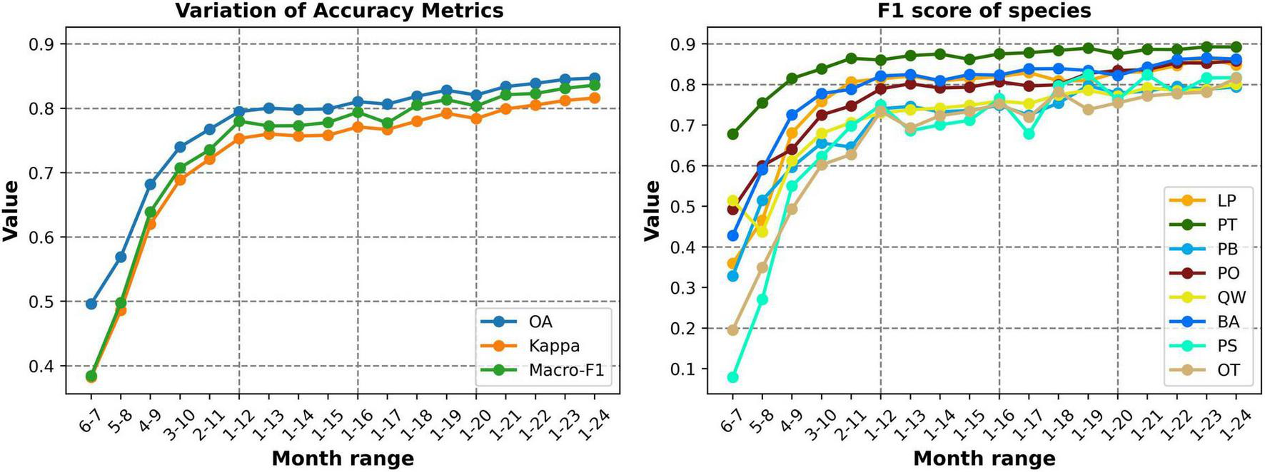
Accuracy and F1 Score variations of different time series construction (1–12 represent January to December 2022, 13–24 represent January to December 2023).
Additionally, we incorporated data from the following year (2023) into the time series, adding one month at a time (13–24 months represent January to December 2023). This approach aimed to determine whether extending the time series beyond an entire growth cycle would enhance accuracy of the model and capture more potential time dependencies and hidden features across annual data. The results showed that extending the length slightly improved classification accuracy, but the gains were much smaller than those seen when the temporal data did not cover a complete growth cycle. Moreover, simply extending the time series does not guarantee improved accuracy. For instance, when the data was extended by an additional 3 months (i.e., 1–15 months) beyond the full year of 2022, here was little improvement in accuracy, with the macro-F1 fluctuating around 0.77 and no increase in OA or Kappa. This indicating that the new data may lack significant additional information. As data from the second year (2023) growing season was incorporated, all metrics continued to grow gradually. Extending the temporal length to 24-months, covering 2 years, all accuracy metrics reached their highest level: OA 0.847, Kappa 0.815, and macro-F1 0.836, Both the accuracy metrics and the F1 score growth curve approached a stable state (Figure 5). We also tested the model using only Sentinel-2 24-months data for classification, and the results showed slightly lower accuracy compared to the combination of two data sources, with an OA of 0.819, Kappa of 0.782, and macro-F1 of 0.805 (confusion matrix in Supplementary Table S2).
The Inverse sampling-intensity weighted method was used to account for potential estimation bias from the spatial distribution of samples. Additional weighted accuracy metrics were calculated, with the confusion matrix shown in Table 2 (Estimated sampling intensity and sample weights distribution in Supplementary Figure S4). The results show a slight decrease in F1 scores for several species, with PO and BA decreasing from 0.85 and 0.86 to 0.81, respectively. There were also adjustments in the overall accuracy metrics, with OA decreasing from 0.847 to 0.834 and macro-F1 dropping from 0.836 to 0.813. These adjustments further improved the reliability of the results, and the overall performance remains satisfactory.
TABLE 2
| Map class | Reference class (samples) | Accuracy | ||||||||||
| LP | PT | PB | PO | QW | BA | PS | OT | UA | PA | F1 score | Weighted-F1 score | |
| LP | 4,349 | 229 | 0 | 4 | 117 | 181 | 15 | 10 | 0.88 | 0.81 | 0.84 | 0.81 |
| PT | 253 | 9,411 | 6 | 43 | 276 | 113 | 74 | 21 | 0.92 | 0.86 | 0.89 | 0.89 |
| PB | 7 | 46 | 2,318 | 277 | 357 | 1 | 0 | 33 | 0.76 | 0.82 | 0.79 | 0.77 |
| PO | 13 | 83 | 270 | 4,472 | 423 | 22 | 0 | 21 | 0.84 | 0.87 | 0.85 | 0.81 |
| QW | 230 | 793 | 177 | 293 | 6,763 | 212 | 29 | 124 | 0.78 | 0.81 | 0.80 | 0.79 |
| BA | 427 | 181 | 0 | 16 | 157 | 4,279 | 23 | 7 | 0.84 | 0.88 | 0.86 | 0.81 |
| PS | 48 | 93 | 1 | 8 | 22 | 22 | 756 | 4 | 0.79 | 0.84 | 0.81 | 0.78 |
| OT | 28 | 57 | 28 | 7 | 167 | 2 | 9 | 1,126 | 0.79 | 0.83 | 0.81 | 0.81 |
| OA = 0.847 | Kappa = 0.815 | macro-F1 = 0.836 | ||||||||||
| OA_w = 0.834 | Kappa_w = 0.791 | macro-F1_w = 0.813 | ||||||||||
Confusion matrix of the classification model using 24-months data.
Confusion matrix along with accuracy metrics, and adjusted metrics using Inverse sampling-intensity weighted (Weighted-F1 Score, OA_w, Kappa_w, and macro-F1_w represent the weighted metrics).
4.3 Forest tree species and biodiversity map
By using 24 months data, the model demonstrated its ability to produce high-quality tree species classification. We applied the trained model to process time series data of all forest pixels, producing a tree species distribution map for the entire region (Figure 6). The map showed good spatial consistency with the forest inventory reference data, demonstrating the reliability of the classification outcomes. The area statistics for each tree species are as follows: Pinus tabuliformis covers the largest area at 2,368.54 km2, followed by Quercus wutaishanica at 760.14 km2. Larix principis-rupprechtii, Pinus bungeana and Betula spp. have similar coverage, with 138.64 km2, 145.14 km2, and 136.29 km2, respectively. Populus spp. occupies a small area of 17.36 km2, while Others (mainly broadleaf) cover 123.53 km2.
FIGURE 6
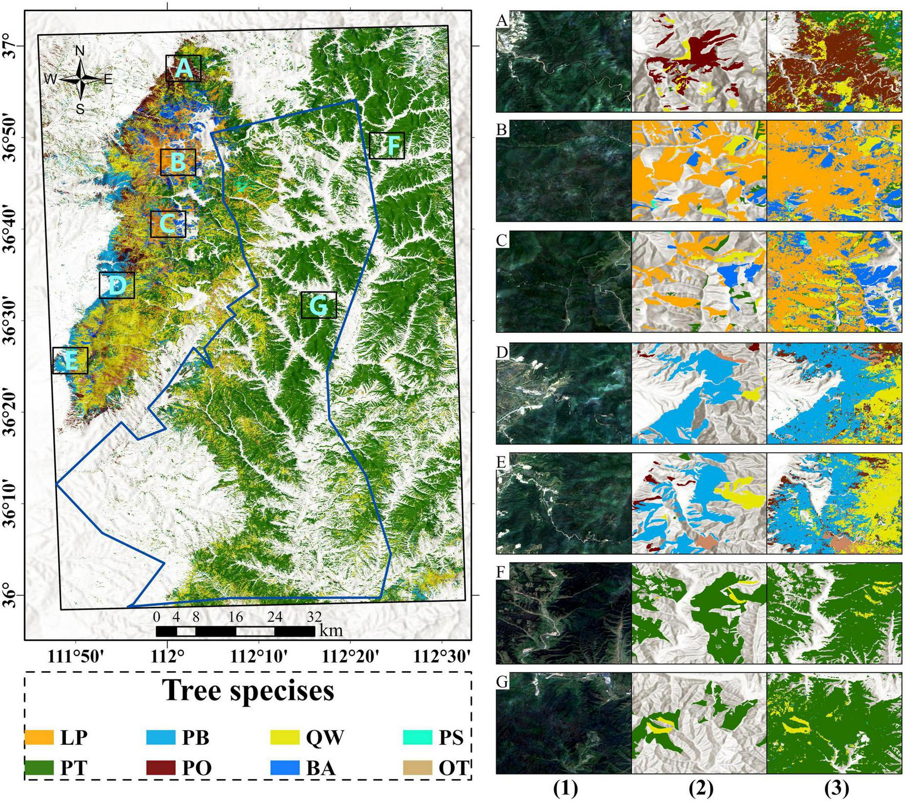
Tree species map of study area. A-G represent the comparison regions with: (1) Sentinel-2 RGB from July 2023 (2) forest investigation map and (3) predicted tree species map.
Three biodiversity indices were calculated using the tree species distribution map and displayed the results (Figure 7). The Species Richness ranges from 1 to 8, indicating the number of tree species within a unit. The Shannon-Wiener Index ranges from 0 to 1.949, with higher values indicating a more complex and even tree species composition. The Simpson’s Diversity Index ranges from 0 to 0.851, with values closer to 1 indicating that most individuals are concentrated in a few species, reflecting lower evenness. These results illustrate the biodiversity of the study area forest, offering insights into the health and resilience of ecosystem.
FIGURE 7
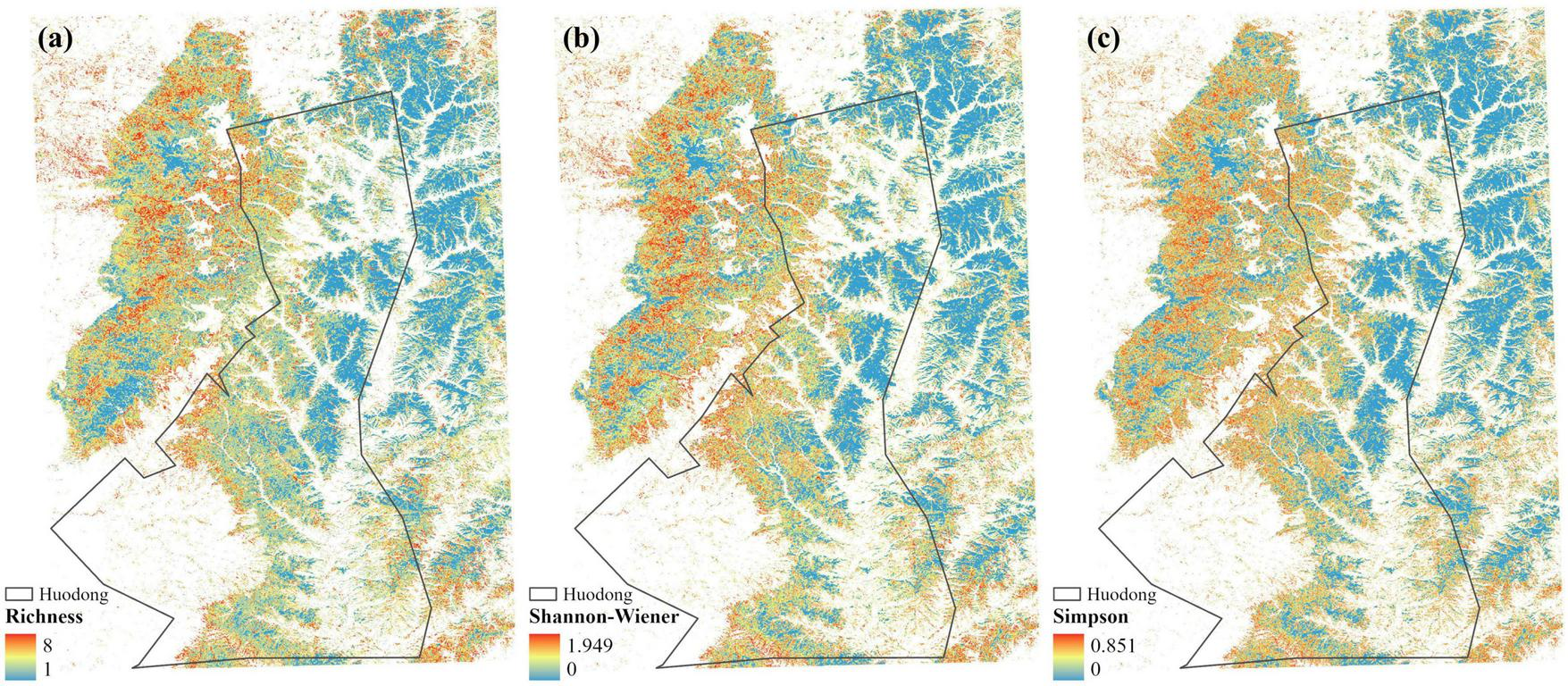
Biodiversity indices of the forest in study area. (A) Species Richness. (B) Shannon-Wiener Index. (C) Simpson’s Diversity Index.
4.4 Key features analysis by statistical methods
The global separability index (SI-global) combines the feature variable separability of various tree species, as shown in Figure 8A, where the intensity of colors indicates differentiation of a feature variable among tree species at a specific time point, reflecting its overall capability to distinguish between species. The results showed that the vegetation indices (e.g., NDVI, GNDVI, NDre1, CIre, etc.) calculated from NIR and red-edge bands demonstrate higher separability, compared to the original band values from satellite sensors. The specific separability indices of all pairs are shown in Supplementary Figure S5. We found that the distinction between deciduous and evergreen species exhibited significantly separability, and extracted the separability index map (Figures 8B,C) for four pairs of tree species (one pair of evergreen species (PT-PO), one pair of deciduous species (LP-BA), and two pairs of mixed deciduous and evergreen species (PT-BA and LP-PT).) The SI heatmaps for same-type species pairs showed low separability, indicating minimal differences in shallow features. In contrast, different species pairs exhibited significant separability, particularly from January to April, October to December, and July to September, with higher index values during these periods. Most deciduous trees are in leafless stages during these periods, leading to significant differences from evergreens in spectral reflectance. These results also highlighted the challenge of distinguishing species with similar phenology.
FIGURE 8
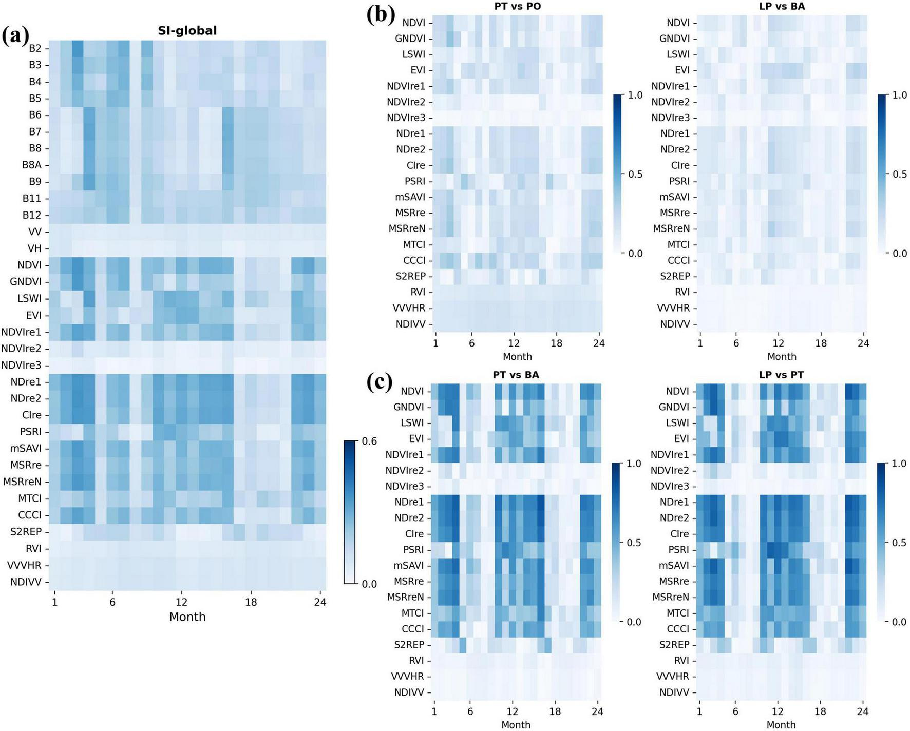
Separability index. The horizontal and vertical axes represent time points (months) and SI of variables, and the color of each cell indicates the separability value. (A) SI-global: Overall separability across all tree species pairs for spectral-temporal features. (B) SI for two pairs of the same tree type (both evergreen or both deciduous). (C) SI for two pairs of different tree types (evergreen vs. deciduous).
PCA was used for dimensionality reduction on the dataset with 33 variables. The results (Figure 9A) showed that the majority of the variance in tree species samples is concentrated in PC1 (37.91%) and PC2 (19.83%). We further analyzed the composition of the two principal components by displaying the distribution of variables (Figure 9B) and the top 10 important variables for each component (Figures 9C,D). Vegetation indices have high contributions in PC1, while optical bands dominate PC2, and SAR data shows minimal contribution in the PCA analysis. In PC1, the red edge indices (NDre1, NDre2, MSReN, MSRre, NDVIre1, Clre) and the optical vegetation indices calculated using near-infrared bands (NDVI, mSAVI, GNDVI, LSWI) contribute significantly, these variables primarily reflect the physiological indicators such as chlorophyll. PC2 is primarily influenced by the original optical satellite bands, reflecting the surface forest canopy’s spectral information, such as leaf color and brightness. To further investigate the importance of each variable at different time points, PCA was performed on monthly data (2023) to assess the contributions to the first two PCs, ranking changes are shown in Supplementary Figure S6, and monthly variable loadings in Supplementary Figure S7. While contributions fluctuated over time, the trend remained consistent with previous analysis. Vegetation indices made the largest contribution to PC1, consistently showing the highest contributions across different time. In contrast, PC2 was primarily influenced by the Sentinel-2 bands.
FIGURE 9
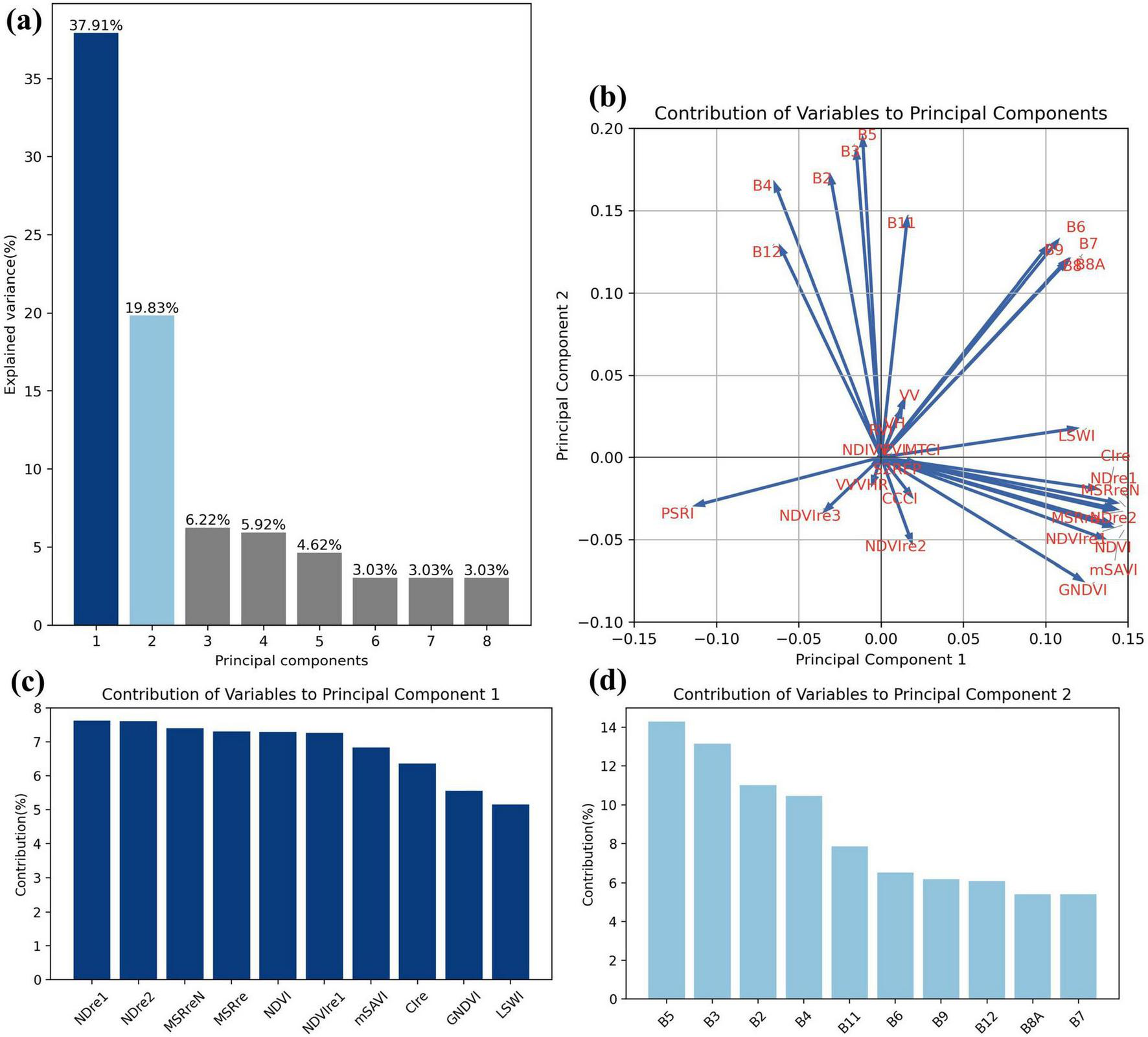
Principal component analysis. (A) Explained variance of first 8 principal components. (B) Biplot of Variable Loadings on PC1 and PC2. (C, D) Contributions of top 10 variables to PC1 and PC2.
4.5 Multidimensional analysis of deep learning classification model
4.5.1 Self-attention weight distribution
The multi-head and layers architecture of the model helps capture information from complex time series data, focusing on different aspects and learning dependencies at multiple levels. In the first layer, weight matrices across tree species are similar, but differences emerge in the second and third layers. We used one species (LP) as an example to illustrate how the model processes information, and all attention weights matrices from the first layer for LP samples was visualized firstly (Figure 10A). In the initial layer, the model aims to extract as much useful information as possible from the input by focusing on various time points. The attention weight matrices showed dispersed attention to help capture global features and some weight matrices exhibited patterns resembling spectral characteristics of tree. For instance, head-1 exhibited high self-attention occurs between 5–9 and 17–21 months (5–9 months of 2023), likely capturing seasonal features linked to leaf growth to shedding periods, as well as the fluctuation of vegetation indices. Conversely, head-3 corresponded to the leafless period of deciduous trees, highlighting the differentiation from evergreens. Head-6 and 7 exhibited attention focused on similar time periods, such as 1–4 and 10–15 or 21–24 months (non-growth seasons), as well as between 4 and 9 months and the corresponding period in the following year. These suggested the model capability to capture correlations, demonstrating its effectiveness in extracting cross-year and seasonal information.
FIGURE 10
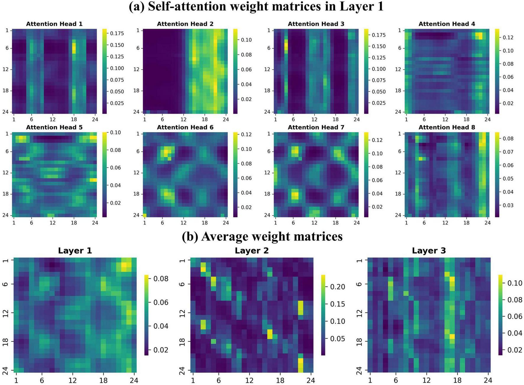
Self-attention weight matrices. The axes represent time points(months). (A) Attention weight distributions for the 8 heads in Layer 1 (LP samples). (B) Average attention weights across three layers.
We averaged the attention weights from all heads in each of the three layers and visualized the resulting matrices to gain a clearer understanding of the model processing mechanism (Figure 10B). In the higher attention layers, the model concentrates on key features and significant time points derived from the shallow features of lower layers, assigning them greater weight. In the second layer, feature extraction converged, with high attention concentrated on fewer time points. The attention weights became more dispersed in next layer, as the model integrates information and revisits valuable features and time points that may have been overlooked. This improvement helps prevent model overfitting to specific features and enhances its generalization, enabling it to more effectively capture both similarities and differences between species, ultimately leading to more reliable identification of tree species.
4.5.2 Dynamics of hidden features separability
400 samples for each specie were selected randomly to illustrate the hidden features extraction process. First, samples with the original 33 features was projected into a two-dimensional space by t-SNE (Figure 11A). The results revealed that the samples from different tree species could not be effectively distinguished, highlighting substantial similarities among the species in the original feature space. This indicated that relying solely on the original features makes it difficult to capture and express the distinct differences between tree species.
FIGURE 11

Visualization of feature separability based on t-SNE. (A) Original features. (B–D) Hidden features from each layer.
Next, the samples data was inputted into the trained classification model, which consists of three Transformer layers with hidden features of 512 dimensions. The hidden representation outputs from each layer was projected and visualized in a two-dimensional space (Figure 11). The hidden feature output of each layer consists of 512-dimensional representations for each sample across all time points. We averaged these features along the time dimension for t-SNE processing and projection into two-dimensional space. As shown in Figure 11, the hidden features extracted and processed through the Transformer layers exhibited more pronounced clustering of similar samples as the model progresses into deeper layers. After being processed by the first layer, a noticeable trend of clustering among similar samples emerged compared to the projection of original features, with LP and PT samples beginning to form clusters. By the second layer, distinct clustering and separation of all tree species became apparent (Figure 11C), and the projection of final layer showed even more pronounced inter-species separation (Figure 11D). The result showed that the samples of deciduous trees, including LP, QW, BA, PS, are closely positioned after dimensionality reduction. Similarly, the evergreen species PB and PO are also near each other.
4.5.3 Soft outputs variations in time series
We tested the impact of time series construction on the classification model in section 4.2, that longer time series data provides additional information beneficial for classification. Additionally, we extracted the soft outputs from models to illustrate how the model confidence in its predictions varies with the increasing length of time series, represented by prediction scores ranging from 0 to 1. The soft outputs for most time series constructions are presented as histograms, divided into 10 intervals of 0.1 (Figure 12A). Details of all tree species prediction scores across these time series constructions are presented in Supplementary Figure S8.
FIGURE 12
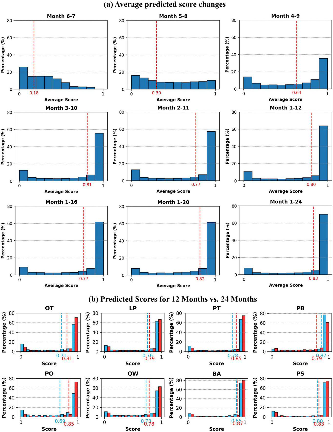
Soft outputs predicted scores. (A) The variation in average predicted scores across different time series compositions (Each value represents the sample percentage within each interval, the red dashed lines represent average score for all species). (B) The comparison of scores between 12-month (blue) and 24-month (red) data.
Similarly, when using only June-July 2022 data, the lack of temporal variation and significant phenological changes resulted in very low prediction scores, indicating inadequate model confidence and failure to identify tree species, with a macro-F1 below 0.4. With data from May to August, a noticeable shift in sample scores occurred, transitioning from a concentration in the lower range to a more even distribution across each interval. The average score also increased, and the proportion of samples with scores above 0.9 grew significantly. When data was extended to cover April to September, the average score reached 0.63, accompanied by a marked increase in high-scoring samples. The soft output prediction scores revealed the rapid accuracy improvement noted in section 4.2 from an internal model perspective, showing that the richer phenological information from April to September greatly enhances the model confidence in identifying tree species. As the time series covered the entire year of 2022, the proportion of samples with prediction scores between 0.9 and 1.0 rose to 64%, with an average score of 0.8, reflecting improved confidence in the classification model outputs.
Incorporating data from the following year into the time series did not significantly raise the average prediction score, but the proportion of the 0.9–1.0 range steadily increased, reaching 70% when covering 2 years, representing a 6% improvement compared to the 1-year results. We compared the prediction scores of each tree species using 1 year (1–12) and 2 years (1–24) of data (Figure 13B), revealing that extending the time series consistently improved the model prediction confidence for nearly all species. However, the average prediction score and the proportion of samples above 0.9 for PB decreased. Despite this, the F1-scores in the two composition were 0.74 and 0.79, confirming improved classification accuracy. The model likely overestimated PB in the 1 year of data, with an average score of 0.9, significantly higher than other species. The extended time series provided additional information, enabling better feature capture, which optimized the scores while improved classification accuracy.
FIGURE 13
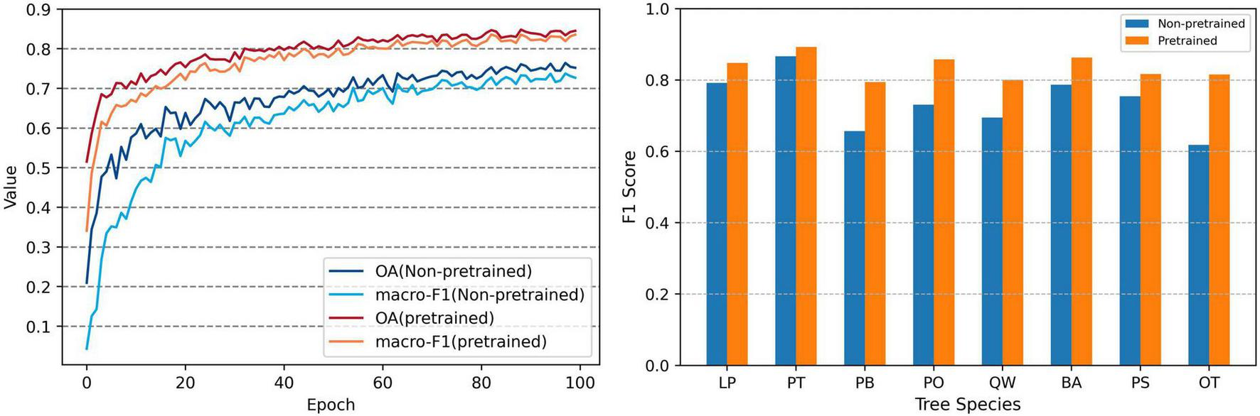
Variation in OA, macro-F1 and F1 Score between Non-pretrained and Pretrained models.
5 Discussion
5.1 Pretraining effects on model performance
The pretrain and fine-tune approach was employed to enhance the classification model ability to identify tree species. We trained a model without pretraining, and compared the changes in OA and macro-F1 during the training process with pretrained model, as well as the final F1 scores for each tree species (Figure 13). The results demonstrated that the model, which was pretrained on forest pixels, significantly improved the accuracy for classification, with noticeable enhancements in the identification accuracy across all species. Additionally, the accuracy curve over training epochs shows that the pretrained model reached the performance ceiling of the non-pretrained model around the 20th epoch, further boosting the accuracy ceiling. The cross-validation results further confirm the enhanced consistency of the pretrained model (Supplementary Figure S9). Existing studies have shown that pretraining models can effectively enhance generalization ability and performance (Jing and Tian, 2021; Misra and Van Der Maaten, 2020). But creating a pretraining task that aligns well with the target task is challenging and requires further research, such as transfer learning strategies and general models (Miller et al., 2024).
5.2 Significance of spectral-temporal features
Extending time series data generally improved classification accuracy for tree species in most cases (Figure 5), highlighting the advantage of using time series images with more varying information (Foerster et al., 2012). Using only June and July data resulted in an OA of just 0.49. Despite the period being the peak growing season for most plants, the shorter series lacked phenological variation, leaving the model to rely almost entirely on spectral reflectance values. Trees with similar phenological traits tend to exhibit highly similar spectral signatures, but key phenological changes are crucial for species identification, and longer time series capturing these shifts provide more information for better differentiation (Liu et al., 2023). Extending the data beyond a full year can still slightly improve accuracy of identifying tree species, but the gains were less significant than adding within-year data, and some additional data may not contribute valuable information. Visualizing the model soft outputs showed that adding an extra year of data boosts prediction confidence, allowing better identification of subtle differences between tree species and optimizing predictions (Figure 12). As time series length increases, classification accuracy for individual tree species and overall performance stabilized at a satisfactory level, and we believe that further extension may not significantly enhance true classification accuracy.
The physiological differences between deciduous and evergreen trees result in distinct spectral reflectance patterns, leading to a more pronounced separability between these two groups. The results indicated that during the leaf fall period, distinct types tree species show significant separability (Figure 8). In contrast, similar growth processes among the same type species lead to insignificant difference in feature values across time series, making accurate identification difficult using only original bands and indices. Many studies emphasize the significance of NIR and Red-edge indices for vegetation research (Frampton et al., 2013; Li et al., 2014), we also found that original bands are less effective for distinguishing between species compared to index variables, even when comparing two distinct types of trees. Vegetation indices effectively highlight differences between tree species by sensitively reflecting physiological indicators like chlorophyll and water content. PCA results also confirm the importance of vegetation index variables (Figure 9), with a high contribution from vegetation indices in the most significant principal component (PC1). PC1 primarily captures seasonal subtle variations in tree physiological characteristics, while PC2, influenced mainly by original bands, reflects differences in leaf color, consistent with previous studies (Schulz et al., 2024). There is variability in the importance of different variables to the principal components across different time periods, due to differences in sensitivity to phenological characteristics at various stages. However, the primary contributors to the two principal components remain the vegetation indices and spectral bands, respectively. We also calculated Pearson’s correlation coefficients among the 33 feature variables to assess inter-variable relationships (Supplementary Figure S10). The results revealed higher correlations and possible redundancy among optical bands with similar wavelengths and their derived vegetation indices, as well as among SAR-derived variables. In contrast, the correlations between variables from the two different sources were generally low. This suggests that adding SAR data to optical inputs may provide complementary information for distinguishing tree species, as the combined data achieved higher tree species classification accuracy compared to using only optical features, with macro-F1 scores of 0.836 and 0.805, respectively. This aligns with previous studies integrating multiple data sources, suggesting that additional information provided by SAR, such as vegetation structural characteristics, may contribute to improved classification performance, which is also reflected in the distinct backscatter profiles across species (Supplementary Figure S2).
5.3 Insights from model visualization
In addition to producing high-accuracy tree species classification maps using deep learning models on SITS, visualizing the model can help us understand its internal processes and bolster its reliability. Multi-head attention weight matrices revealed the model behavior in capturing information from various aspects of the input time series, including key phenological changes and periods of features similarity (section 4.5.1). The model employed nonlinear transformations and multi-head self-attention mechanisms to continuously extract and integrate features, enhancing class-relevant information while diminishing irrelevant features. This process evolves the input features into a more abstract and separable form, illustrating the significant advantage of deep learning in processing time series data and capturing information (Vaswani et al., 2017; Xu et al., 2020).
Projecting hidden features from each model layer and the original features, clearly illustrated how low-level inputs are transformed into high-level representations that effectively distinguish tree species (section 4.5.2). In the shallow layers of model, input retains low-level features closely tied to their original forms, leading to mixed distributions of different tree species. As the model progresses to deeper layers, it captures features of increasing complexity most relevant to the categories, transforming hidden features to project different tree species into a more distinct feature space for precise separation (Goodfellow et al., 2016). We also found that the samples of deciduous species cluster closely after projection, as do the evergreen species, which aligns with our feature analysis, indicating smaller differences and reduced separability among similar tree species. In the final output layer, we observed significant inter-class separation among samples, indicating that deeper phenological features are captured by the model. Similarities lead to close proximity in the projected space, while differences create distinct clusters.
5.4 Tree species distribution and biodiversity
The tree species distribution map and forest biodiversity results revealed a certain correlation between tree species distribution and elevation (Figure 6). Pinus tabuliformis dominates the forests of study area, primarily located in the low-elevation regions of eastern Taiyue Mountain and near the Huodong coal mining area, which also exhibited lower levels of biodiversity. According to information gathered from forestry departments, this trend may be attributed to large-scale plantings in the 1980s and reclamation plantings after mining activities, leading to a lack of species diversity. In contrast, Taiyue Mountain is predominantly covered by primary forests, which exhibited a richer species composition and higher levels of biodiversity. Many studies have found that primary forests have higher species diversity and biomass than planted and second-growth forests (Cavanaugh et al., 2014; Shirima et al., 2015). The second largest tree species in the study area, Quercus wutaishanica, is mainly in the southern part of Taiyue Mountain. Pinus bungeana is distributed along the western edge of Taiyue, forming a continuous strip, while Platycladus orientalis is located in the northwest, near the Pinus bungeana. Larix principis-rupprechtii and Quercus wutaishanica are concentrated in the high-altitude central region. The distribution and biodiversity data of tree species provided crucial information and effective support for forest ecosystem management and ecological research. For mining areas, where forest harvesting and replanting is a recurring process, it is crucial to implement more comprehensive and diverse planting strategies to protect and enhance both forest biodiversity and carbon sequestration capacity.
6 Conclusion
In this study, we presented a deep learning-based method with SITS to achieve high-precision forest tree species and tree species biodiversity mapping. By pretraining the model on unlabeled forest pixels, the model performance was significantly enhanced, resulting in faster convergence and higher accuracy compared to the non-pretrained. Increasing the time series length improves classification accuracy, indicating that incorporating multi-temporal information across different phenological stages benefits tree species classification. While adding data beyond a full year can still improve model performance and confidence to some extent, the improvement is neither guaranteed nor limitless. Most vegetation indices, such as NDVIre, NDre and MSRre, are more sensitive than satellite bands in reflecting differences between tree species during key phenological stages, particularly between evergreen and deciduous trees. The Transformer-based model effectively captures and processes these key features, enabling accurate species classification. The methodologies designed for tree species classification and multidimensional interpretation, facilitate efficient species identification and enhance understanding of the integration of SITS and deep learning. This is valuable for related ecological research, and more studies are needed in the future to further explore the combination of SITS and deep learning to gain a clearer understanding of ecosystems.
Statements
Data availability statement
The original contributions presented in the study are included in the article/Supplementary material, further inquiries can be directed to the corresponding author.
Author contributions
JT: Writing – original draft, Formal Analysis, Software, Conceptualization, Writing – review & editing, Methodology. JL: Conceptualization, Supervision, Funding acquisition, Writing – review & editing. TM: Methodology, Validation, Writing – review & editing, Investigation. XY: Writing – review & editing, Data curation, Validation, Investigation. ZH: Writing – review & editing, Data curation, Validation.
Funding
The author(s) declare that financial support was received for the research and/or publication of this article. This work was supported by the National Key Research and Development Program of China (2022YFE0127700).
Conflict of interest
The authors declare that the research was conducted in the absence of any commercial or financial relationships that could be construed as a potential conflict of interest.
Generative AI statement
The authors declare that no Generative AI was used in the creation of this manuscript.
Publisher’s note
All claims expressed in this article are solely those of the authors and do not necessarily represent those of their affiliated organizations, or those of the publisher, the editors and the reviewers. Any product that may be evaluated in this article, or claim that may be made by its manufacturer, is not guaranteed or endorsed by the publisher.
Supplementary material
The Supplementary Material for this article can be found online at: https://www.frontiersin.org/articles/10.3389/ffgc.2025.1599510/full#supplementary-material
References
1
Asner G. P. Jones M. O. Martin R. E. Knapp D. E. Hughes R. F. (2008). Remote sensing of native and invasive species in Hawaiian forests.Remote Sens. Environ.1121912–1926. 10.1016/j.rse.2007.02.043
2
Blickensdörfer L. Oehmichen K. Pflugmacher D. Kleinschmit B. Hostert P. (2024). National tree species mapping using Sentinel-1/2 time series and German National Forest Inventory data.Remote Sens. Environ.304:114069. 10.1016/j.rse.2024.114069
3
Camps-Valls G. Bandos Marsheva T. V. Zhou D. (2007). Semi-Supervised graph-based hyperspectral image classification.IEEE Trans. Geosci. Remote Sens.453044–3054. 10.1109/TGRS.2007.895416
4
Cavanaugh K. C. Gosnell J. S. Davis S. L. Ahumada J. Boundja P. Clark D. B. et al (2014). Carbon storage in tropical forests correlates with taxonomic diversity and functional dominance on a global scale.Glob. Ecol. Biogeogr.23563–573. 10.1111/geb.12143
5
Chen H. Qi Z. Shi Z. (2022). Remote sensing image change detection with transformers.IEEE Trans. Geosci. Remote Sens.601–14. 10.1109/TGRS.2021.3095166
6
De Bruin S. Brus D. J. Heuvelink G. B. M. Van Ebbenhorst Tengbergen T. Wadoux A. M. J.-C. (2022). Dealing with clustered samples for assessing map accuracy by cross-validation.Ecol. Inform.69:101665. 10.1016/j.ecoinf.2022.101665
7
Dou P. Shen H. Li Z. Guan X. (2021). Time series remote sensing image classification framework using combination of deep learning and multiple classifiers system.Int. J. Appl. Earth Obs. Geoinform.103:102477. 10.1016/j.jag.2021.102477
8
Fassnacht F. E. Latifi H. Stereńczak K. Modzelewska A. Lefsky M. Waser L. T. et al (2016). Review of studies on tree species classification from remotely sensed data.Remote Sens. Environ.18664–87. 10.1016/j.rse.2016.08.013
9
Fassnacht F. E. Neumann C. Forster M. Buddenbaum H. Ghosh A. Clasen A. et al (2014). Comparison of feature reduction algorithms for classifying tree species with hyperspectral data on three central european test sites.IEEE J. Sel. Top. Appl. Earth Obs. Remote Sens.72547–2561. 10.1109/JSTARS.2014.2329390
10
Felton A. Petersson L. Nilsson O. Witzell J. Cleary M. Felton A. M. et al (2020). The tree species matters: Biodiversity and ecosystem service implications of replacing Scots pine production stands with Norway spruce.Ambio491035–1049. 10.1007/s13280-019-01259-x
11
Foerster S. Kaden K. Foerster M. Itzerott S. (2012). Crop type mapping using spectral–temporal profiles and phenological information.Comput. Electron. Agric.8930–40. 10.1016/j.compag.2012.07.015
12
Frampton W. J. Dash J. Watmough G. Milton E. J. (2013). Evaluating the capabilities of Sentinel-2 for quantitative estimation of biophysical variables in vegetation.ISPRS J. Photogramm. Remote Sens.8283–92. 10.1016/j.isprsjprs.2013.04.007
13
Fu B. He X. Yao H. Liang Y. Deng T. He H. et al (2022). Comparison of RFE-DL and stacking ensemble learning algorithms for classifying mangrove species on UAV multispectral images.Int. J. Appl. Earth Obs. Geoinform.112:102890. 10.1016/j.jag.2022.102890
14
Goodfellow I. Bengio Y. Courville A. (2016). Deep learning, adaptive computation and machine learning.Cambridge, MA: The MIT Press.
15
Hemmerling J. Pflugmacher D. Hostert P. (2021). Mapping temperate forest tree species using dense Sentinel-2 time series.Remote Sens. Environ.267:112743. 10.1016/6/j.rse.2021.112743
16
Hermosilla T. Bastyr A. Coops N. C. White J. C. Wulder M. A. (2022). Mapping the presence and distribution of tree species in Canada’s forested ecosystems.Remote Sens. Environ.282:113276. 10.1016/j.rse.2022.113276
17
Hu Q. Sulla-Menashe D. Xu B. Yin H. Tang H. Yang P. et al (2019). A phenology-based spectral and temporal feature selection method for crop mapping from satellite time series.Int. J. Appl. Earth Obs. Geoinform.80218–229. 10.1016/j.jag.2019.04.014
18
Ienco D. Gaetano R. Dupaquier C. Maurel P. (2017). Land cover classification via multitemporal spatial data by deep recurrent neural networks.IEEE Geosci. Remote Sens. Lett.141685–1689. 10.1109/LGRS.2017.2728698
19
Immitzer M. Neuwirth M. Böck S. Brenner H. Vuolo F. Atzberger C. (2019). Optimal input features for tree species classification in central Europe based on multi-temporal sentinel-2 data.Remote Sens.11:2599. 10.3390/rs11222599
20
Interdonato R. Ienco D. Gaetano R. Ose K. (2019). DuPLO: A dual view point deep learning architecture for time series classification.ISPRS J. Photogramm. Remote Sens.14991–104. 10.1016/j.isprsjprs.2019.01.011
21
Jing L. Tian Y. (2021). Self-Supervised visual feature learning with deep neural networks: A survey.IEEE Trans. Pattern Anal. Mach. Intell.434037–4058. 10.1109/TPAMI.2020.2992393
22
Jolliffe I. T. Cadima J. (2016). Principal component analysis: A review and recent developments.Philos. Trans. R. Soc. Math. Phys. Eng. Sci.374:20150202. 10.1098/rsta.2015.0202
23
Kollert A. Bremer M. Löw M. Rutzinger M. (2021). Exploring the potential of land surface phenology and seasonal cloud free composites of one year of Sentinel-2 imagery for tree species mapping in a mountainous region.Int. J. Appl. Earth Obs. Geoinform.94:102208. 10.1016/j.jag.2020.102208
24
Kumar P. Kumar A. Patil M. Hussain S. Singh A. N. (2024). Factors influencing tree biomass and carbon stock in the Western Himalayas.India. Front. For. Glob. Change6:1328694. 10.3389/ffgc.2023.1328694
25
Lechner A. M. Foody G. M. Boyd D. S. (2020). Applications in remote sensing to forest ecology and management.One Earth2405–412. 10.1016/j.oneear.2020.05.001
26
Li F. Miao Y. Feng G. Yuan F. Yue S. Gao X. et al (2014). Improving estimation of summer maize nitrogen status with red edge-based spectral vegetation indices.Field Crops Res.157111–123. 10.1016/j.fcr.2013.12.018
27
Li K. Zhao W. Peng R. Ye T. (2022). Multi-branch self-learning Vision Transformer (MSViT) for crop type mapping with Optical-SAR time-series.Comput. Electron. Agric.203:107497. 10.1016/j.compag.2022.107497
28
Lindner M. Maroschek M. Netherer S. Kremer A. Barbati A. Garcia-Gonzalo J. et al (2010). Climate change impacts, adaptive capacity, and vulnerability of European forest ecosystems.For. Ecol. Manag.259698–709. 10.1016/j.foreco.2009.09.023
29
Lipton Z. C. (2018). The mythos of model interpretability.Commun. ACM6136–43. 10.1145/3233231
30
Liu X. Xie S. Yang J. Sun L. Liu L. Zhang Q. et al (2023). Comparisons between temporal statistical metrics, time series stacks and phenological features derived from NASA Harmonized Landsat Sentinel-2 data for crop type mapping.Comput. Electron. Agric.211:108015. 10.1016/j.compag.2023.108015
31
Löw F. Michel U. Dech S. Conrad C. (2013). Impact of feature selection on the accuracy and spatial uncertainty of per-field crop classification using support vector machines.ISPRS J. Photogramm. Remote Sens.85102–119. 10.1016/j.isprsjprs.2013.08.007
32
Melnyk O. Manko P. Brunn A. (2023). Remote sensing methods for estimating tree species of forests in the Volyn region, Ukraine.Front. For. Glob. Change6:1041882. 10.3389/ffgc.2023.1041882
33
Miller L. Pelletier C. Webb G. I. (2024). Deep learning for satellite image time-series analysis: A review.IEEE Geosci. Remote Sens. Mag.1281–124. 10.1109/MGRS.2024.3393010
34
Misra I. Van Der Maaten L. (2020). “Self-Supervised learning of pretext-invariant representations,” in Proceedings of the 2020 IEEE/CVF Conference on Computer Vision and Pattern Recognition (CVPR), (Seattle, WA: IEEE).
35
Ngo Y.-N. Ho Tong, Minh D. Baghdadi N. Fayad I. (2023). Tropical forest top height by GEDI: From sparse coverage to continuous data.Remote Sens.15:975. 10.3390/rs15040975
36
Pedregosa F. Varoquaux G. Gramfort A. Michel V. Thirion B. Grisel O. et al (2011). Scikit-learn: Machine learning in python.J. Mach. Learn. Res.122825–2830. 10.5555/1953048.2078195
37
Pelletier C. Webb G. Petitjean F. (2019). Temporal convolutional neural network for the classification of satellite image time series.Remote Sens.11:523. 10.3390/rs11050523
38
Peng X. Chen Z. Chen Y. Chen Q. Liu H. Wang J. et al (2021). Modelling of the biodiversity of tropical forests in China based on unmanned aerial vehicle multispectral and light detection and ranging data.Int. J. Remote Sens.428858–8877. 10.1080/01431161.2021.1954714
39
Rußwurm M. Korner M. (2017). “Temporal vegetation modelling using long short-term memory networks for crop identification from medium-resolution multi-spectral satellite images,” in Proceedings of the 2017 IEEE Conference on Computer Vision and Pattern Recognition Workshops (CVPRW), (Honolulu, HI: IEEE).
40
Rußwurm M. Körner M. (2020). Self-attention for raw optical satellite time series classification.ISPRS J. Photogramm. Remote Sens.169421–435. 10.1016/j.isprsjprs.2020.06.006
41
Samek W. Binder A. Montavon G. Lapuschkin S. Muller K.-R. (2017). Evaluating the visualization of what a deep neural network has learned.IEEE Trans. Neural Netw. Learn. Syst.282660–2673. 10.1109/TNNLS.2016.2599820
42
Schulz C. Förster M. Vulova S. V. Rocha A. D. Kleinschmit B. (2024). Spectral-temporal traits in Sentinel-1 C-band SAR and Sentinel-2 multispectral remote sensing time series for 61 tree species in Central Europe.Remote Sens. Environ.307:114162. 10.1016/j.rse.2024.114162
43
Shirima D. D. Totland Ø Munishi P. K. T. Moe S. R. (2015). Relationships between tree species richness, evenness and aboveground carbon storage in montane forests and miombo woodlands of Tanzania.Basic Appl. Ecol.16239–249. 10.1016/j.baae.2014.11.008
44
Somers B. Asner G. P. (2014). Tree species mapping in tropical forests using multi-temporal imaging spectroscopy: Wavelength adaptive spectral mixture analysis.Int. J. Appl. Earth Obs. Geoinform.3157–66. 10.1016/j.jag.2014.02.006
45
Somers B. Delalieux S. Verstraeten W. W. Van Aardt J. A. N. Albrigo G. L. Coppin P. (2010). An automated waveband selection technique for optimized hyperspectral mixture analysis.Int. J. Remote Sens.315549–5568. 10.1080/01431160903311305
46
Tan K. Hu J. Li J. Du P. (2015). A novel semi-supervised hyperspectral image classification approach based on spatial neighborhood information and classifier combination.ISPRS J. Photogramm. Remote Sens.10519–29. 10.1016/j.isprsjprs.2015.03.006
47
van der Maaten L. Hinton G. (2008). Visualizing data using t-SNE.J. Mach. Learn. Res.92579–2605.
48
Vaswani A. Shazeer N. Parmar N. Uszkoreit J. Jones L. Gomez A. N. et al (2017). “Attention is all you need,” in Proceedings of the 31st International Conference on Neural Information Processing Systems (NeurIPS 2017), (California, CA: Long Beach).
49
Wang R. Gamon J. A. (2019). Remote sensing of terrestrial plant biodiversity.Remote Sens. Environ.231:111218. 10.1016/j.rse.2019.111218
50
White J. C. Coops N. C. Wulder M. A. Vastaranta M. Hilker T. Tompalski P. (2016). Remote sensing technologies for enhancing forest inventories: A review.Can. J. Remote Sens.42619–641. 10.1080/07038992.2016.1207484
51
Xiao J. Chevallier F. Gomez C. Guanter L. Hicke J. A. Huete A. R. et al (2019). Remote sensing of the terrestrial carbon cycle: A review of advances over 50 years.Remote Sens. Environ.233:111383. 10.1016/j.rse.2019.111383
52
Xu J. Yang J. Xiong X. Li H. Huang J. Ting K. C. et al (2021). Towards interpreting multi-temporal deep learning models in crop mapping.Remote Sens. Environ.264:112599. 10.1016/j.rse.2021.112599
53
Xu J. Zhu Y. Zhong R. Lin Z. Xu J. Jiang H. et al (2020). DeepCropMapping: A multi-temporal deep learning approach with improved spatial generalizability for dynamic corn and soybean mapping.Remote Sens. Environ.247:111946. 10.1016/j.rse.2020.111946
54
Yang B. Wu L. Liu M. Liu X. Zhao Y. Zhang T. (2024). Mapping forest tree species using sentinel-2 time series by taking into account tree age.Forests15:474. 10.3390/f15030474
55
You N. Dong J. (2020). Examining earliest identifiable timing of crops using all available sentinel 1/2 imagery and google earth engine.ISPRS J. Photogramm. Remote Sens.161109–123. 10.1016/j.isprsjprs.2020.01.001
56
Yuan Y. Lin L. (2021). Self-Supervised pretraining of transformers for satellite image time series classification.IEEE J. Sel. Top. Appl. Earth Obs. Remote Sens.14474–487. 10.1109/JSTARS.2020.3036602
57
Zhang Y. Wang N. Wang Y. Li M. (2023). A new strategy for improving the accuracy of forest aboveground biomass estimates in an alpine region based on multi-source remote sensing.GIScience Remote Sens.60:2163574. 10.1080/15481603.2022.2163574
58
Zhao W. Qu Y. Zhang L. Li K. (2022). Spatial-aware SAR-optical time-series deep integration for crop phenology tracking.Remote Sens. Environ.276:113046. 10.1016/j.rse.2022.113046
59
Zhong L. Hu L. Zhou H. (2019). Deep learning based multi-temporal crop classification.Remote Sens. Environ.221430–443. 10.1016/j.rse.2018.11.032
60
Zhou Z.-H. (2018). A brief introduction to weakly supervised learning.Natl. Sci. Rev.544–53. 10.1093/nsr/nwx106
Summary
Keywords
tree species classification, remote sensing, deep learning, biodiversity, Sentinel-1/2
Citation
Tan J, Li J, Ma T, Yan X and Huo Z (2025) Leveraging Sentinel-1/2 time series and deep learning for accurate forest tree species mapping. Front. For. Glob. Change 8:1599510. doi: 10.3389/ffgc.2025.1599510
Received
25 March 2025
Accepted
19 June 2025
Published
04 July 2025
Volume
8 - 2025
Edited by
Fernando J. Aguilar, University of Almería, Spain
Reviewed by
Emilio Ramírez-Juidías, University of Seville, Spain
Rajesh Vanguri, Sapienza University of Rome, Italy
Updates
Copyright
© 2025 Tan, Li, Ma, Yan and Huo.
This is an open-access article distributed under the terms of the Creative Commons Attribution License (CC BY). The use, distribution or reproduction in other forums is permitted, provided the original author(s) and the copyright owner(s) are credited and that the original publication in this journal is cited, in accordance with accepted academic practice. No use, distribution or reproduction is permitted which does not comply with these terms.
*Correspondence: Jing Li, lijing@cumtb.edu.cn
Disclaimer
All claims expressed in this article are solely those of the authors and do not necessarily represent those of their affiliated organizations, or those of the publisher, the editors and the reviewers. Any product that may be evaluated in this article or claim that may be made by its manufacturer is not guaranteed or endorsed by the publisher.