Changing climate may drive large shifts in vegetation zones of Oregon, USA

Anticipating plausible future ecosystem states is necessary for effective ecosystem management. We use climate analog-based impact models and a co-production process with land managers to project future vegetation changes for the state of Oregon, United States, (2041–2070, RCP 8.5) at a management-relevant spatial resolution (270-m). We explore multiple analog-based methodologies, evaluate analog model performance with contemporary validation, and leverage climate analogs to assess projection uncertainty by quantifying areas where multiple vegetation trajectories are plausible under a single climate scenario. We find that analog-based models performed well at reproducing landscape-level vegetation composition, and moderately well at reproducing vegetation at the pixel level. Our results suggest that 64% of the study area will experience future climate conditions that support different potential natural vegetation types and 59% will experience climates corresponding with different potential plant physiognomic types, compared to reference-period conditions. We project a 60% reduction of mesic conifer-dominated forests with transitions to mixed evergreen forest types. We also project losses to dry forests, cold forests and parklands, with commensurate expansions of shrublands, grasslands, and geographic redistribution of dry forest types. We find that in many areas, several vegetation trajectories are plausible under a single climate scenario. Finally, we provide guidance for using future vegetation projections and uncertainty outputs in management decisions using the Resist-Accept-Direct (RAD) adaptation framework.

1 Introduction

Evidence of climate-driven ecosystem transformations is accumulating globally (Sullivan et al., 2022; Manrique-Ascencio et al., 2024; Ma et al., 2024) and across the western United States (US). In the western U.S., low-elevation dry forests are transitioning to non-forest following high-severity disturbance, due to both increasingly inhospitable climate and a lack of seed sources which limit tree reestablishment post-disturbance (Coop et al., 2020; Davis et al., 2019; Boag et al., 2020; Guiterman et al., 2022). Additionally, dry forests are experiencing increased rates of drought-related tree mortality (Hartmann et al., 2022), which may lead to significant changes in dominant species composition and to changes in physiognomic type (Allen and Breshears, 1998; Rodman et al., 2022). Further, subalpine forests (Higuera et al., 2021) are experiencing novel fire regimes which may lead to novel vegetation recovery trajectories and decreasing resilience (Whitman et al., 2019; Turner et al., 2019).

Given the pace and scale of these transformations (Coop et al., 2020), natural resource managers increasingly have to consider climate-driven impacts to the ecosystems they manage. Effective resource management requires knowing which locations are at risk of change, and what kinds of changes are likely (Krosby et al., 2020). In this study, we model potential climate-driven vegetation transitions across 22 million hectares within the state of Oregon. We chose to focus on the state of Oregon given the diversity of ecosystem types within the state from dry shrublands to mesic coastal forests, the presence of strong climate gradients, and willing co-production partners that span federal, state, and non-government organizations. Our contribution is threefold: (1) we use a novel approach to project potential vegetation transitions based on climate analogs and leverage the approach's unique characteristics to develop estimates of projection uncertainty; (2) we project impacts at a spatial resolution (270 m pixels) relevant for management; and (3) we co-produce this study with natural resource managers of federal, state, tribal, and private lands, to ensure the results are actionable for management decision-making.

Anticipating climate impacts to Oregon's ecosystems is crucial for understanding how ecosystem services (e.g., carbon storage, habitat provision for threatened and endangered species, timber production, and recreation) and economies associated with these services may change in the future. Previous mechanistic modeling studies highlight the potential for widespread climate-driven vegetation changes in Oregon including loss of subalpine forests (Halofsky et al., 2022b; Kim et al., 2018), shifts from mesic to warm and xeric forests (Halofsky et al., 2022a), and transition of conifer-dominated forests to mixed (conifer and broad-leaf) forests (Halofsky et al., 2022a,b; Case et al., 2020; Sheehan et al., 2015), woodlands and shrublands (Kim et al., 2018). These mechanistic model projections are broadly consistent with observational studies and empirical models that report compositional changes to forests and potential physiognomic vegetation type transitions within Oregon (Boag et al., 2020; Dodson and Root, 2013; Bennett et al., 2023; Serra-Diaz et al., 2018).

In this study, we use analog impact models (AIMs), an empirical modeling approach, which are increasingly employed for climate-impact projections (e.g., Dobrowski et al., 2021; Coffield et al., 2021; Chaudhary et al., 2023; Povak and Manley, 2024; Yegorova et al., 2025). AIMs rely on reverse climate analogs—places that today have the projected future climate of a focal location. Reverse analogs (“analogs” from here on) answer the question, “where does the future climate of my location of interest occur today?” (Hamann et al., 2015, Figure 1a). AIMs make projections of future plausible ecological states by intersecting locations of reverse analogs with state variables (e.g., vegetation data), and summarizing the vegetation conditions at reverse analog locations (Figure 1b). For a detailed discussion of analogs and AIMs see Yegorova et al. (2025).

Figure 1

Figure 1. Reverse climate analogs (a) are locations in the reference period with climates similar to the projected future climate at location X (focal location). Analog impact models (AIM) (b) use information about state variables found at reverse analog locations (e.g., vegetation type) to project potential changes to those state variables at the focal location under a future climate. In this simplified example there are six reverse analogs identified. The six analog locations, in total, represent three different vegetation types (b). The most commonly supported vegetation type is used as a primary (or plurality) projection. However, secondary and tertiary projections can provide relevant information for resource managers. We use information about the proportion of votes for the plurality projection to assess projection uncertainty. For example, if the proportion of votes for the primary and secondary vegetation types is similar, we consider both types as plausible vegetation projections.

AIMs possess several characteristics that contribute to our understanding of potential vegetation changes. First, AIMs are spatial models—they can capture spatially structured information because reverse analogs tend to be found proximally to their focal locations (Hamann et al., 2015; Yegorova et al., 2025). In contrast, non-spatial models, including most regression approaches, start with geographic information (e.g., georeferenced plots), translate it into aspatial information (e.g., climate space), and then transfer model forecasts back into geographic space. This approach to modeling loses information about spatial patterns of occupancy, neighborhood effects, and other spatially structured processes that are not explicitly included in a model. In contrast, spatial models can account for the influence of location, which succinctly summarizes the effects of spatially structured processes regardless of whether they are included in the model directly. Spatial models usually outperform non-spatial models at reconstructing existing ecological patterns (Miller et al., 2007) and tend to provide more conservative projections of climate impacts, due to the influence of occupancy patterns and spatial inertia (Crase et al., 2014; Swanson et al., 2013). Second, AIMs can identify locations expected to develop novel climates (Williams et al., 2007)—climates not currently found in the region of interest, or even globally. In the paleorecord, novel climates are associated with the emergence of novel ecological communities (Ordonez et al., 2016). Therefore, identifying the locations of expected novel climates allows one to highlight areas where future community composition may have no contemporary analog. Third, AIMs provide a means to visualize and communicate uncertainty or alternative outcomes in model projections, which is crucial for adaptation planning (Beier et al., 2017). Specifically, AIMs highlight areas where the model is either incapable of distinguishing between climates of different vegetation types or where multiple alternative vegetation projections are plausible under the projected climate (Figure 1b, see Section 2). Reporting multiple alternative projections enables users to better understand model outputs and judge which projections are resulting from unlikely model assumptions or unrepresented processes.

Although the scope of climate adaptation products has rapidly grown in the last three decades, the uptake of these products by resource managers has not kept pace (Lemos et al., 2012). For example, Krosby et al. (2020) show that in the Pacific Northwest there are multiple climate-relevant tools available that are underutilized by resource managers. Co-production, or collaborative development of science with potential end users, can increase the use of science products (Kirchhoff et al., 2013; Jagannathan et al., 2020). Consequently, we co-produced this study with representatives of natural resource management entities in Oregon in an attempt to make the outputs relevant and accessible to end-users. Our co-production process was characterized by iterative collaborative engagement over the course of 2 years through a series of meetings and workshops. Our co-production partners influenced data inputs to our model, interpreted model outputs, and shaped the format of the final products. Additionally, we attempt to improve our study usability by interpreting our results using the Resist-Accept-Direct framework (RAD, Schuurman et al., 2020). The RAD framework acknowledges that the traditional management approach of resisting incoming ecological changes may not be feasible or sufficient in the face of ongoing ecological transformations, and expands consideration of management options to include intentional acceptance of change or intentionally directing ecosystems into a new state (Schuurman et al., 2020). The RAD framework is increasingly used in natural resource management (Resist-Accept-Direct Framework, 2025), and our intent in presenting our results in the RAD framework is to increase our results' usability.

In this study, we model vegetation distribution for the mid-21st century (2041–2070, RCP 8.5) for the state of Oregon. We compare reference and projected vegetation distributions to highlight areas of vegetation stability and areas vulnerable to climate-driven transition. We assess projection uncertainty and highlight areas where multiple alternative vegetation states are likely. Lastly, to improve the usability of our results, we provide an example of how our model outputs can inform management actions under the Resist-Accept-Direct (RAD) framework (Schuurman et al., 2020), which is increasingly used to frame management decision-making in the face of changing climate (e.g., Davis et al., 2023). Our study contributes to a growing body of climate impact projections in the Pacific Northwest with a novel, analog-based, approach, and a co-production process. Our findings are intended to improve the ability of government agencies and other interested parties (i.e., non-governmental organizations) to manage landscapes in an era of rapid change.

2 Methods

2.1 Co-production process

We worked with The Nature Conservancy-Oregon (TNC) to recruit co-production participants from an extensive network of TNC's partners. TNC's role in the process was crucial, as their established relationships with managers facilitated the relationship development necessary for a co-production process. Interested parties were invited to an in-person workshop that aimed to identify common goals among the co-production partners, familiarize partners with the project methods, and get partner buy-in. The initial in-person workshop was followed by five virtual meetings. The formal co-production process concluded with an in-person workshop that presented project results and a virtual meeting releasing project data outputs. Overall, 41 managers and scientists representing 14 different entities participated in at least one meeting. Supplementary Table S1 summarizes participating organizations.

Our co-production process followed Beier et al.'s (2017) recommended co-production practices. The initial in-person workshop focused on identifying partners' information needs and on understanding how our proposed project could fill those needs (recommended practice #3). We iteratively addressed the assumptions of the model (recommended practice #5) by dedicating co-production meetings to examining components of the modeling process (such as vegetation data inputs, climate definitions, modeling methodology), and to questioning early project outputs. Finally, as a group, we focused on evaluating and communicating the uncertainty in our results (recommended practice #7). Two of our outputs are dedicated to assessing uncertainty of modeling results.

2.2 Climate data

Following Dobrowski et al. (2021), we characterized climate using four variables: annual evapotranspiration (AET), climatic water deficit (CWD), average daily maximum temperature of July (T_max7), and average daily minimum temperature of December (T_min12). Water balance variables (AET and CWD) summarize simultaneous water and energy availability, are strongly associated with vegetation distribution patterns (Stephenson, 1998), and are commonly used to model vegetation distribution (Kane et al., 2015; Lutz et al., 2010). T_min12 and T_max7 characterize climate seasonality, are ecologically relevant correlates of vegetation distribution (Woodward, 1987) and provide a more specific definition of climate compared to average seasonal temperature (Mahony et al., 2017).

Reference climate is represented by annual data for the 1981–2010 period, downscaled from monthly 4 km resolution gridMet data (Abatzoglou, 2013) to 90 m resolution using generalized additive models with latitude, longitude, and elevation as covariates. The future climate is represented by the annual data for the 2041–2070 period, downscaled to 90 m resolution from the MACA v2 dataset, trained with GridMet (Abatzoglou and Brown, 2012). Future data represent an ensemble mean for 20 global circulation models from the Climate Model Intercomparison Project, all using inputs from the RCP 8.5 scenario (Taylor et al., 2012). The downscaled climate data were developed for the state of Oregon and a 100 kilometer buffer around the state to allow for analog searches beyond the border of the state (further information on climate dataset development in Supplementary Data Sheet 1, Supplement 1).

2.3 Vegetation data

We surveyed co-production partners to identify a vegetation product that would best meet their needs for management applications. No single product satisfied all partners, yet the majority preferred the US Forest Service Region 6 Potential Natural Vegetation (PNV) dataset (Simpson et al., in press, data and documentation available at https://teui-region6-usfs.hub.arcgis.com/pages/pnv). The PNV dataset consists of vegetation zones (“vegzones”) which represent the late seral species assemblages that could develop in the absence of disturbance (Simpson et al., in press). Each vegzone is named after a dominant or co-dominant late seral species in that community. Vegzones are further differentiated into “subzones” representing climate variations within a given vegzone (wet, very wet, warm dry, etc.). PNV is modeled using the gradient nearest neighbor imputation, based on climate, geomorphology, geology and floristics (PNV USFS. PNV., n.d. USFS). Preliminary description of PNV modeling process can be found at the PNV Region 6 web-site (PNV. USFS). The relationships between vegezones used in this study and the four climate variables can be seen in Supplementary Figure S9. Land managers consider vegzones and subzones to be discrete vegetation types with unique ecological dynamics. Managers use PNV vegzones and subzones to infer characteristics such as productivity, habitat potential and expected responses to disturbances, and to frame desired conditions at several scales. While the naming convention is based upon late seral vegetation, there is no assumption that vegetation is currently in or will in the future reach late seral assemblage. Similarly it is also not assumed that the late seral assemblages used to name vegzones represent an optimal or desired ecological state. PNV data have a 30-meter resolution.

In the 1981–2010 reference period, there were 22 PNV vegzones and 76 subzones in the state of Oregon (after excluding developed, rock, water, and wetland-associated subzones). We performed vegetation projections at the subzone level, and then aggregated these to two coarser levels of thematic resolution: (1) vegzones, and (2) “physiognomic types” defined by our co-production partners. The physiognomic types included: subalpine parklands (“parklands” from here on and in PNV vegzone descriptions), cold forest, mesic forest, dry forest, very dry forest, dry woodland, mixed evergreen forest, hardwoods, shrublands, and grasslands. The crosswalk between PNV subzones and physiognomic types is presented in Supplementary Table S2.

The PNV dataset covers Oregon, Washington and California, but does not include Idaho and Nevada, where many climate analogs for eastern and central Oregon are found. To make projections into these areas, we crosswalked Landfire's 2020 biophysical settings (BpS) product (Rollins, 2009) to PNV vegzone and physiognomic vegetation type (Supplementary Table S3). BpS data have a 30-meter resolution. We report results at the vegzone and physiognomic type levels, and we provide the data for subzone-level projections to our project partners.

For both vegetation and climate datasets, we removed pixels classified as developed, water, rock, and wetland vegetation, as the distribution of these cover types is primarily influenced by factors other than climate. AIMs perform a comparison between a focal pixel's climate and the climate of all potential analogs, that is all pixels on the landscape. We found that at 90 meter resolution (the resolution of the climate data), the search for analogs was too computationally expensive. To alleviate the computational burden of finding climate analogs, we aggregated vegetation data to 270 m resolution by assigning the modal vegetation value of the eighty one 30 m pixels within the aggregated 270 m pixel. Climate data were aggregated to 270 m resolution using the mean value of the nine pixels comprising each 270 m pixel. We performed spatial data manipulation in R 4.3.2, using the terra package (Hijmans, 2023).

2.4 Analog impact model (AIM)

To find climate analogs, we performed pairwise comparison of the projected future climate at each focal location to reference climate at potential reverse analog locations (Figure 1a). We limited the pool of potential analogs to a randomly selected sample of 500,000 pixels (10% of the study area) for computational feasibility. We measured dissimilarity between a focal climate and potential analog climates using Mahalanobis distance (MD). MD calculates the distance in climate space (defined by our four climate variables) between mean climates (averaged over a 30 year period) of focal and potential analog locations, and scales it by the interannual variability of the focal climate (Mahony et al., 2017).

Following Mahony et al. (2017), we set a cut-off value for analogous climates at two standard deviations (2σ) of the focal climate's interannual climate variability. Potential analog climates that are more than 2σ away from their focal climate are considered non-analogous and are not used in projections. We converted MDs between the focal and potential analog climates into σ units and retained the 100 reverse analogs with the lowest σ values. Some focal locations did not have 100 analogs with σ <2; in those cases, we retained all that did and reported the total number retained.

To project plausible future vegetation at a focal pixel, we intersected the locations of the 100 reverse analogs with the vegetation data to produce a distribution of potential vegetation types deemed plausible at the focal site in the future (Figure 1b). We explored two approaches for assigning a vegetation type to each focal location: a “plurality” approach (e.g., Dobrowski et al., 2021) and a “sampling” approach. In the plurality approach, the vegetation type with the greatest number of analog votes is projected at a focal pixel (primary projection in Figure 1b). In addition to maintaining the plurality vote, we also retained information on the secondary and tertiary vegetation types with the most votes, as a means to understand variation in potential outcomes (Figure 1b). We report the number of analog votes for the primary vegetation class as a measure of the likelihood of alternative vegetation outcomes. The plurality approach is expected to have a smoothing effect on the overall projected vegetation composition, as it biases the projections toward more common vegetation types because rare vegetation types are unlikely to gain the highest number of votes. To address this issue, we also developed a “sampling” approach: we took a single random sample (n = 1) from the vegetation projected by 100 reverse analogs and used it as the projection of future vegetation at the focal location. Selecting a single sample is expected to weight vegetation projections by their relative prevalence among 100 analogs, while also retaining a degree of stochasticity which allows for less common vegetation types to be represented.

2.5 Projection uncertainty

We used two measures of projection uncertainty: (1) mean σ of reverse analogs, which represents climate dissimilarity between the focal and analog climates and (2) analog agreement, which we interpret as the possibility for multiple vegetation trajectories under a single future climate (Dobrowski et al., 2021). To assess the climatic dissimilarity of analogs we calculated the mean σ value of the analogs used for vegetation projections. We considered projections made with lower mean σ to have lower uncertainty compared to those with larger σ values because the historical climate at analog locations better matches the projected future climate of the focal location.

We quantified analog agreement as the number of votes received by the primary vegetation type at each focal pixel (Figure 1b). Low values of analog agreement can arise from two potential sources: future climate can support multiple vegetation types, or our model is unable to meaningfully discern between climates associated with multiple vegetation classes. Either possibility indicates projection uncertainty. High values of analog agreement, on the other hand, suggest that the future climate condition used in this model is primarily associated with a single vegetation type. We use these measures of uncertainty to suggest management approaches under the RAD framework.

2.6 Contemporary validation

To assess the skill of the AIM, we asked how well our model reproduced existing vegetation patterns. This approach is commonly used to assess the skill of mechanistic (Halofsky et al., 2013; Kim et al., 2018) and empirical species distribution models (see Rehfeldt et al., 2006) and has been previously used with AIMs (e.g., Parks et al., 2019; Pugh et al., 2016). We conducted contemporary validation on a subset of 100,000 randomly chosen focal pixels (3% of the study area). For these pixels, we selected 100 contemporary analogs—locations whose reference climate is analogous to that of a focal location's reference climate; simply, places that today have similar climates.

The best contemporary analogs of a focal pixel are often pixels adjacent to that focal location, because climate is self-similar in space (i.e., is spatially structured). This spatial aggregation of contemporary analogs is likely to capture the effects of not only climate but also other spatially-structured variables because biotic and abiotic variables are also spatially autocorrelated (Legendre and Fortin, 1989). However, reverse analogs are unlikely to match the spatial distribution of contemporary analogs. To avoid inflating contemporary validation performance due to spatial proximity of contemporary analogs, we explored the effect of using an exclusion radius of 85, 122, and 183 kilometers around each focal pixel. These distances represent the 10th, 25th, and 50th percentile of mean distances to reverse analogs, respectively.

We examined the AIM's performance in two ways: (1) how well it reproduced vegetation types at the scale of individual pixels, and (2) how well it reproduced state-level vegetation composition (i.e., proportions of landscape occupied by vegetation types). For the pixel-level accuracy assessment, we report raw accuracy (i.e., percent of pixels correctly classified) and Cohen's Kappa (Cohen, 1960). Cohen's Kappa accounts for the number of classes and their relative prevalence and is considered a more balanced measure of classification accuracy. For landscape-level composition accuracy, we calculated the Bray-Curtis dissimilarity index (McCune et al., 2002) between AIM-reconstructed and reference-period landscape composition. The Bray-Curtis index takes into account both the vegetation types and their relative prevalence to assess the difference between two communities. It ranges from 0 to 1. An AIM-derived contemporary prediction identical to the observed community would have a score of 0, while a prediction with no vegetation classes in common with the observed community would have a score of 1. To provide context for interpreting these performance measures, we compared results from the AIM validation model to a null model in which “null analogs” were based on 100 random locations (outside of the same exclusion radius) to estimate a focal pixel's reference period PNV.

3 Results

3.1 Climatic changes

Contemporary CWD for Oregon averages 201 mm with SD of 100 mm. Average CWD increased by 44 mm (climate became more water-limited) between the reference and future time periods. This change represents approximately half a standard deviation of reference period CWD for the state of Oregon. The largest increases in CWD (80–90 mm) are projected for south-western and western Oregon (Supplementary Figure S1a), areas which have some of the lowest reference-period CWD in the state. On average, AET is projected to increase by 16 mm (mean reference AET value 484 mm), with the greatest increases in high elevation areas that are currently energy-limited: the crest of the Cascades and Wallowa mountains (Supplementary Figure S1b). The mean projected T_min12 increase is 2.1 °C (mean reference T_min12 value is 3.7 °C) and mean projected T_max7 increase is 3.6 °C (from mean reference T_max7 of 28.6 °C, Supplementary Figures S1c, d).

3.2 Vegetation projections

AIMs model climate redistribution, and assume that vegetation is in pseudo-equilibrium with climate, as do other empirical models (Araújo et al., 2005). Consequently, we describe “vegetation transitions” when in fact a more accurate description is that there is a “transition of climates associated with physiognomic type/vegzone X.” We herein use both phrases interchangeably.

We organize and summarize our results by vegetation (physiognomic types and vegzones) and level 3 ecoregions within the state (Omernik, 1987) (Figure 2). We report results for all thematic resolutions (vegzone and physiognomic type) from the sampling approach, unless otherwise noted. Visualizations of results form the plurality approach, can be found in Supplementary Figures (Supplemental Data Sheet 1), as referenced in the main text.

Figure 2

Figure 2. Study area (Oregon) location on the map of the United States (US), and level 3 ecoregions in the state of Oregon. The upper left map shows Oregon's location within the US. The main map shows level 3 ecoregions in the state of Oregon (Omernik, 1987). We use level 3 ecoregions to describe projection patterns in the results.

3.3 Physiognomic types

By the future 2041–2070 period, 59% of the study area is projected to support a different physiognomic type than in the reference period (Figures 3A, B, 4). Climates associated with conifer-dominated physiognomic types are projected to shrink from 64% to 27% of the study area (Figure 4). This reduction is driven by declines in mesic coniferous forests (from 24% to 9%), as well as dry forests (from 18 to 13%), very dry forests (8% to 1%) and woodlands (9% to 7%). Climates that support mesic forest in the reference period are projected to transition to mixed evergreen (coniferous and broadleaf) forest types, which increase from 2% to 19% of the study area. Climates supporting dry forest types are projected to transition to climates supporting shrublands, which expand from 33% to 46% of the study area, and grasslands, which increase from 0.5% to 3.1% of the study area (Figure 4). Climates associated with cold forests and parklands are projected to nearly disappear, changing to mesic and dry forest types (Figure 4). Dry forests and dry woodlands decrease less compared to other coniferous forest types, by 29% and 17%, respectively, but they are projected to redistribute on the landscape. Only 24% of dry forests and 11% of dry woodlands are projected to remain stable between the reference and future period.

Figure 3

Figure 3. Distribution of physiognomic types in the reference period (1981–2010) (A) and projected physiognomic types in the future period (2041–2070) using the sampling (B) method. White areas in maps (A, B) indicate masked out vegzones: developed, wetland and water classes. Black lines are level 3 ecoregions (Omernik, 1987).

Figure 4

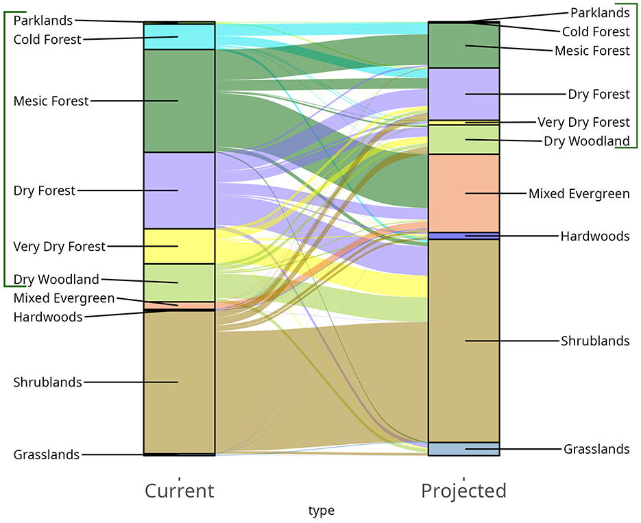
Figure 4. Current and projected landscape composition (based on the sampling approach), and composition changes. The height of each color column indicates the proportion of the study area occupied by climate associated with the physiognomic type in the reference (“Current”) or future time period (“Projected”). The width of the flow lines and their trajectory indicate the proportion of a given physiognomic type that remains in the same class or changes to a different class. The brackets on the left and right highlight conifer-dominated physiognomic types: parklands, cold forest, mesic forest, dry forest, very dry forest, and dry woodland.

Primary vegetation projections from the plurality approach are qualitatively similar to the sampling approach at the physiognomic type level (Table 1), however the plurality approach tended to over-represent the most common physiognomic types (Table 1) and vegzones, at the expense of less common vegetation types.

Table 1

Table 1. Comparison of reference and projected landscape composition at the physiognomic type level for sampled and plurality methods (see Section 2 for further description).

3.4 Vegzone projections

The proportion of the landscape expected to transition increases with thematic resolution: 63% of the landscape is projected to shift to a climate associated with a different vegzone. The vegzone components of physiognomic type groupings do not necessarily respond uniformly (Supplementary Figure S2). For example, dry forests are projected to decrease on the landscape. However, two of the dry forest vegzones, Jeffrey pine and Douglas-fir, are projected to expand (Supplementary Figure S2), while the rest of dry forest vegzones, Ponderosa pine, Pinyon-Juniper and White Fir-Grand Fir, are projected to decrease in area (Supplementary Figure S2). On the other hand, all components of the subalpine parklands and cold forest are projected to decline. Parklands, Lodgepole Pine, Mountain Hemlock and Pacific Silver Fir, Subalpine Fir-Engelmann Spruce, and Red Fir-Shasta Fir are projected to decrease by more than 90% relative to the reference period (Supplementary Figure S2). These are regionally the coldest vegzones, which occupy a relatively small area in the reference period (Supplementary Figure S2). See Supplementary Figures S3, S4 for maps representing vegzone-level projected vegetation distribution.

3.5 Geographic distribution of transitions

Transitions of the climate associated with physiognomic types are projected throughout the state of Oregon (Figure 5). In western Oregon, future climate is expected to support warmer and drier forest types (e.g., mixed evergreen forest vs. mesic coniferous forest, and mesic coniferous forest vs. cold forest). In the East Cascades and Blue Mountains, future climate is expected to support drier forest types or non-forested physiognomic types. Areas where future climate is projected to support the same vegetation as contemporary climate (“Stable”−41% of the study area) include the north end of the Coast Range, limited areas of the Cascades, and the shrublands of eastern Oregon. Definitions of transition types can be found in Supplementary Table S4.

Figure 5

Figure 5. Areas of projected vegetation transitions and transition types. Black lines are level 3 ecoregions (Omernik, 1987). Supplementary Table S4 describes how individual vegzone transitions translate to this taxonomy. White areas indicate areas masked out of the analysis: developed, wetland, and water classes.

3.6 Projection uncertainty

Overall, we found high climate similarity between projected future climates and reference climates (Figure 6A). We did not find strong evidence of emergence of novel climates: 99.94% of the pixels in the study area had at least 100 analogs with σ <2. The mean σ value of analogs was 0.13 and 93% of pixels had σ less than 0.5. Southwest Oregon is an exception to this, with mean σ greater than 1 (Figure 6A).

Figure 6

Figure 6. Measures of uncertainty. Mean Sigma (σ, climatic dissimilarity) of the best one hundred analogs (A). Blue areas show high climate similarity between the future and reference climates, red areas—less so. Analog agreement (B)—the number of analog votes for the plurality vegetation type (i.e., most common vegetation type selected by 100 analogs). We consider projections made at locations with greater analog agreement (purple areas) more certain than at areas with lower analog agreement (gray and red areas). White areas in the map represent excluded vegetation (wetlands) and cover types (developed areas, rock, wetlands, and water). Black lines are level 3 ecoregions (Omernik, 1987).

Mean analog agreement was 78% at the physiognomic type level and 71% at the vegzone level. Analog agreement varied across the state (Figure 6B). Large swaths of Western Oregon, Western Cascades and portions of the Basin and Range ecoregions had high analog agreement (>50 votes for plurality vegetation, approximately 90% of the area), suggesting that conditions are projected to be suitable for a single physiognomic type. By contrast, portions of the Blue Mountains ecoregion, parts of the Oregon Coast, parts of the Cascades, and the Basin and Range ecoregion had low analog agreement (<50 votes, approximately 10% of the study area), indicating multiple plausible future vegetation types.

In areas of high projection uncertainty due to low analog agreement, considering secondary and tertiary analog projections in addition to the primary one is necessary (Supplementary Figure S10c). The plurality method provides information about primary and secondary plausible vegetation types. For example, in the Blue Mountains ecoregion, climates that are projected to support mostly shrubland may also support dry forests, woodlands and grasslands (Figures 7B, C). A map of secondary plurality vegetation projections for the state can be found in Supplementary Figure S7. Vegzone-level analog agreement, and primary and secondary plurality projections can be found in Supplementary Figure S4.

Figure 7

Figure 7. Reference vegetation (A), and primary (B) and secondary (C) physiognomic type projections from the plurality method for the Blue Mountains ecoregion. Analog agreement can be used to identify areas, where projected climate may support multiple vegetation types (areas of low analog agreement). Primary and secondary projections provide information about alternative vegetation types possible in these “low agreement” areas. White areas in the map represent excluded vegetation and cover types. Grey areas (marked “NA” in the legend) indicate locations where no alternative vegetation type was projected (C). Black lines are level 3 ecoregions (Omernik, 1987).

3.7 Contemporary validation

We report model skill for the plurality and the sampling approaches to highlight their difference and relative strengths. Overall, the sampling approach had higher skill at reproducing reference period landscape-level composition (Bray Curtis dissimilarity index = 0.13) compared to the plurality approach (Bray Curtis dissimilarity index = 0.21, Figure 8, Supplementary Figure S8, Supplementary Tables S5, S6). In contrast, the plurality approach showed higher skill at reproducing vegetation types at the individual pixel scale (Cohen's Kappa 0.49) compared to the sampling approach (Cohen's Kappa 0.42, Supplementary Table S5). At the landscape level, the plurality approach reduced the overall number of vegzones from 21 to 20, overrepresenting more common vegetation types and underrepresenting less common ones (Figure 8). Normalized difference between actual and reconstructed vegzone-level compositions can be viewed in Supplementary Figure S8. In contrast, the sampling approach reproduced all of the reference period vegzones and captured less common vegetation types (Figure 8). Both the plurality and the sampling approach overestimated the prevalence of shrublands and underestimated prevalence of dry forests and woodlands (Douglas-fir, Ponderosa pine and Pinyon-Juniper-Cypress vegzones in Figure 8).

Figure 8

Figure 8. Reference period and AIM-reconstructed landscape composition at the PNV vegzone thematic level using the sampling and the plurality approach. The Bray-Curtis dissimilarity scores comparing actual and reconstructed compositions can be viewed in Supplementary Table S5. The Y axis represents the number of pixels occupied by a vegzone in the validation subset (100,000 randomly chosen pixels). Normalized differences between actual and AIM-reconstructed landscape compositions can be viewed in Supplementary Figure S8.

At the pixel level, model skill varied by exclusion distances (better performance with smaller exclusion radii), and with the thematic resolution of the vegetation data (better performance at coarser thematic resolutions, Supplementary Table S6). The probability of reproducing focal vegetation correctly at the pixel level increased with the number of votes for the plurality vegetation type (Supplementary Figure S5). Both the plurality and the sampling methods outperformed the null models at the pixel level (by 0.39 and 0.33 Cohen's kappa units, vegzone thematic resolution). At the landscape level, the null sampling approach performed well, as expected. The null sampling model takes a random sample of the landscape, which allows it to reproduce landscape composition well. However, the null sampling method performs poorly at reproducing the correct vegetation at the pixel level (Supplementary Table S6). The null plurality approach was significantly outperformed by the sampling and the plurality AIM models at the landscape level. More details on the landscape level and pixel level comparisons can be found in Supplementary Tables S5, S6.

4 Discussion

Climate change has the potential to alter vegetation composition and the geographic distribution of vegetation types in Oregon. The AIM-based projections suggest that by the second half of the 21st century (2041–2070), 59% of Oregon's landscape will have climates associated with a different plant physiognomic type (Figures 3, 4). The largest transitions are projected for areas with climates currently associated with (1) mesic coniferous forests, with 50% of these areas transitioning to climates of mixed evergreen forests, and (2) dry forest types, with 23% of these areas transitioning to climates associated with shrublands. The projections for vegetation transition are even higher at finer thematic resolutions, with 63% of the landscape projected to transition to a different vegzone (Supplementary Figure S4). These projected transitions are distributed throughout the state, indicating widespread vulnerability to climate-driven vegetation turnover (Figure 5).

4.1 Regional patterns of transition and stability

To be useful, projections of vegetation transitions have to be interpreted with respect to their uncertainty, including the possibility for multiple alternative vegetation states under a future climate. In this and subsequent sections, we interpret our findings by comparing our projections to those from other studies and by considering measures of projection uncertainty.

We project loss of high elevation, energy-limited, forest types which is in agreement with other modeling studies for this region (Halofsky et al., 2013; Case et al., 2020; Halofsky et al., 2022b). We also project that nearly all climates associated with cold forests and parklands will be replaced by climates favoring mesic forests at the crest of the Cascades, and dry forest at the crest of Blue Mountains.

Our projections for western Oregon are consistent with results from several mechanistic-modeling studies for this area, which suggest that climate will shift to favor mixed evergreen (conifer and broadleaf-dominated) forest instead of conifer-dominated mesic forest (Sheehan et al., 2015; Case et al., 2020; Turner et al., 2015; Yospin et al., 2015; Halofsky et al., 2022b). This transition may manifest as a change in the relative dominance of species that already co-occur in some locations. For example, Douglas-fir is a co-dominant species in both mixed evergreen and mesic conifer forest types. The mixed evergreen physiognomic type has a significant component of broadleaf evergreen and deciduous species, while the mesic conifer type has a significant presence of western hemlock. Therefore, transitions between conifer and the mixed evergreen types may manifest as a replacement of more mesic coniferous species with broadleaf evergreen and deciduous trees and shrubs, while retaining a component of Douglas-fir codominance.

In contrast, our projections for forest to non-forest transition in the Blue Mountains and East Cascades (Figure 5) contribute to a divergent set of results from modeling and observational studies for these regions. While we project the loss of climates associated with forests, the low analog agreement in these areas (Figure 6B) indicates that future climate may allow for multiple vegetation types. In many of these low agreement areas, the second most-supported vegetation type is dry forest or dry woodland (Pinyon-Juniper-Cypress, Douglas-Fir, Ponderosa and Jeffrey Pine vegzones; Figures 7B, C). Additionally, our model validation results show that AIMs tend to overestimate the extent of shrubland vegzone and underestimate dry- and very dry forest vegzones (Douglas-fir, Pinyon-Juniper-Cypress, and Ponderosa pine, Figure 8), suggesting that some of the forest-to-shrubland transitions may be overestimated. Other modeling and observational studies also diverge in their forecasts of future vegetation for these ecoregions. For example, mechanistic-model based studies project continued dominance of coniferous forests (Kim et al., 2018; Sheehan et al., 2015; Halofsky et al., 2013; Case et al., 2020). In contrast, an empirical model suggests conifer regeneration may be unlikely, especially following high severity fire, in much of the Blue Mountains and the lower elevations of the East Cascades (Davis et al., 2023). Finally, an observational study by Boag et al. (2020) reported a lack of post-fire conifer regeneration in low-elevation forests of the Blue Mountains that burned at high severity, suggesting that a forest-to-non forest transition may be underway in these areas. We interpret these divergent findings to mean that the future of forests in the Blue Mountains and East Cascades is uncertain. The future climate of these ecoregions might bring dry forests to the cusp of transition, where high severity disturbance may trigger a conversion to a different physiognomic type. In the face of an uncertain future, actively reducing forest vulnerability to high severity disturbances through thinning and prescribed burning may prolong forest dominance in these areas (Davis et al., 2024).

Our results suggest multiple areas of vegetation stability, despite changing climate (Figure 5). However, these projections of vegetation stability should be interpreted with caution and consideration to the underlying assumptions of our modeling approach. In southwest Oregon, the mixed evergreen physiognomic type is projected to remain stable despite changing climate. However, higher-than-average σ values for these projections indicate a looser correspondence between focal and analog climates, reducing our confidence in these projections. The projected stability in the Basin and Range ecoregion, on the other hand, may be an artifact of insufficiently resolved shrubland data and our inability to account for non-native species invasion dynamics. Large parts of the Basin and Range ecoregion had reverse analogs in Idaho and Nevada, areas outside of the Region 6 PNV dataset. For these locations, we crosswalked BpS vegetation classes to PNV vegzones (see Section 2). The Basin and Range ecoregion is projected to continue to support shrubland vegzone, however the stable shrubland vegzone may mask transitions among the eight shrubland subzones. For example, Creutzburg et al. (2015) project a climate-driven increase in moist shrub steppe and fluctuating levels of dry shrub steppe in the second half of the 21st century. Additionally, the shrub steppe in this ecoregion are threatened by ongoing annual grass invasion (Smith et al., 2022; Creutzburg et al., 2022) and subsequent fire regime changes (Bradley et al., 2018; Balch et al., 2013) which often lead to permanent shrubland-to-grassland conversion (Chambers et al., 2019). Our projections do not represent invasion dynamics, and therefore may mistakenly project continued shrub dominance when a conversion to annual grassland may be more likely.

4.2 Projection uncertainty

Information about uncertainty of modeled results provides key context for their interpretation and application. Overall, neither climatic novelty (σ > 2) nor poor climatic match between focal and analog climates (σ approaching 2) was a significant source of uncertainty in our study (Figure 6A). The lack of evidence of novel climates emerging by 2041–2070 is contrary to other studies (Dobrowski et al., 2021; Mahony et al., 2017). There are two potential reasons we did not find novel climates. First, our vegetation projections excluded large valleys (e.g., Willamette Valley, Upper Klamath Basin) because they are classified as “developed” vegetation types. However, large valleys are the most likely locations to develop novel climates (Mahony et al., 2017; Dobrowski et al., 2021). These low topographic positions are already the warmest locations on the landscape, which means that finding an even warmer reference period climate to match the projected climates in these areas is unlikely. Second, the fine spatial resolution of climate data in this study allowed us to find analogs in locations where coarser climate data may overlook them. Fine grain climate data are associated with reduced projections of climate novelty (Hamann et al., 2015; Ordonez et al., 2016; Dobrowski and Parks, 2016; Heikkinen et al., 2020). This reduced novelty is likely due to the increased variability captured by fine grain climate data.

We highlight the southwest corner of Oregon as an area of weaker climatic similarity between focal and analog climates (Figure 6A), and therefore an area of less certain vegetation projections, compared to the rest of the state. High σ values for projections in southwest Oregon may be a result of our data limitations: we searched for analogs in the state of Oregon and a 100 kilometer buffer around it. Extending the search further south along the California coast may yield more climatically similar analogs (lower σ). Mahony et al. (2017) also report high σ values for southwest Oregon, despite their continent-wide search for analogs. However, Mahony et al. (2017) used coarser climate data in their study (4 × 4 km²) compared to ours (270 × 270 m²), which leaves the possibility for more climatically similar analogs to be found with finer-grain climate data (Ordonez et al., 2016; Heikkinen et al., 2020). Alternatively, this area's future climate may become increasingly novel, suggesting that southwest Oregon may develop novel plant assemblages.

We interpret low analog agreement as an indicator of projection uncertainty. This interpretation is supported by our contemporary validation results: greater analog agreement is associated with a greater probability of correctly reproducing reference period vegetation at the pixel level (Supplementary Figure S5). This uncertainty can originate from two sources: the future climate projected for a particular pixel could support multiple vegetation classes, e.g., climates supporting vegetation ecotones (e.g., Allen and Breshears, 1998; Gosz, 1993) or it could indicate the model's inability to meaningfully distinguish among climates of multiple vegetation classes. Distinguishing between these possibilities may require pixel-by-pixel or region-by-region consideration of primary, secondary, and tertiary vegetation projections. However, both possibilities suggest projection uncertainty.

While the mean analog agreement for the study area was high (78%), it varied geographically and showed distinct areas of high and low projection uncertainty (Figure 6B). Significant portions of the Blue Mountains, East Cascades, Basin, and Range ecoregions and portions of Oregon coast are areas where the projected physiognomic vegetation type is one of several possible. In these areas, any single vegetation projection is associated with heightened uncertainty, and evaluating alternative vegetation types is necessary to understand possible development trajectories.

Analog agreement and climate dissimilarity should be considered in tandem to characterize the uncertainty of projections. For example, southwestern Oregon has high analog agreement, and high climate dissimilarity (σ > 1). In this case, the high climate dissimilarity of analogs undermines the certainty associated with high analog agreement, and the overall vegetation projection should be considered uncertain.

Overall, we recommend interpreting AIM outputs at a spatial unit that represents an aggregate of individual pixels (for example, subwatershed, watershed, ecoregions) as opposed to interpreting individual pixels. While we provide projections at a fine spatial grain, the moderate pixel-level validation success (Cohen's Kappa 0.35–0.49, Supplementary Table S6) suggests caution for interpreting pixel-level results. However, AIM showed skill at reproducing overall vegetation composition (Figure 8, Supplementary Table S5). Therefore, we interpret the projection for climate driven vegetation composition shifts with more confidence than the exact locations of these shifts.

4.3 Other sources of uncertainty and caveats

Our projections of vegetation changes are subject to multiple assumptions, which additionally contribute to the uncertainty of our projections. Our projections are based on the mean of an ensemble of climate models under the high emissions pathway (RCP 8.5) and therefore overlook the uncertainty associated with climate model selection and other emissions pathways. Climate uncertainty can be an equal or greater contributor, compared to model uncertainty, in species distribution modeling (Wenger et al., 2013) and analog-based modeling specifically (Grenier et al., 2013; Yegorova et al., 2025). A more robust approach is to consider climate projections from several models and under different emission pathways to represent the uncertainty of future climate scenarios (e.g., Lawrence et al., 2021). We suggest interpreting the results of our study accordingly, as one of potentially many vegetation futures. One way to fill in this information gap is to consider our study in conjunction with other efforts that do consider several climate scenarios (e.g., Kim et al., 2018). Additionally, our projections are for the 2041–2070 period, and therefore do not consider climate trajectories and vegetation projections for the last quarter of the century. Our interpretations implicitly assume climate stabilization following the projection period, this stabilization is unlikely given current emissions and climate projections.

As with other empirical models, our study assumes that vegetation shifts will follow climate. However, whether and when the vegetation types will change depends on many factors, including catalyzing disturbance (Crausbay et al., 2017; Thom et al., 2017), management history, species' dispersal capacity (Corlett and Westcott, 2013), competition (Liang et al., 2018) and other biotic interactions (Brown and Vellend, 2014) all of which modulate plant response to climate. Long-lived species, such as trees, can persist for decades or centuries in climates that are no longer favorable to continued establishment of seedlings (Dobrowski and Swanson, 2015; Serra-Diaz et al., 2018). In such cases, disturbance events that kill mature individuals (fire, forest harvest, drought, insect infestation etc.) can catalyze an abrupt transition from one vegetation type to another. Management actions aimed at reducing severe disturbances may significantly delay climate-driven vegetation conversions. Nevertheless, with changing climate and fire regimes, observations of forest to non-forest shifts are accumulating across the western US (Coop et al., 2020; Davis et al., 2019) and in low-elevation forests of Oregon specifically (Boag et al., 2020; Dodson and Root, 2013). To colonize habitat opened by disturbance, species must be able to disperse, establish and successfully compete. However, the mean distance to analog in our study (180 km, Supplementary Figure S6) corresponds to a climate velocity of 3 km/year, exceeding dispersal distances for many plant species (Corlett and Westcott, 2013). Finally, we make projections with vegzones, a necessary simplification to communicate the effects of climate change. The use of vegetation classes (vegzones) assumes species assemblages will respond to climate deterministically, which is not supported by the paleorecord (Jackson and Blois, 2015; Rapacciuolo et al., 2014; Jackson and Overpeck, 2000). However, vegzones are intended to communicate site climatic potential, and thus vegzones are particularly suitable for analog-based modeling, as both are defined based on climate.

4.4 Considering plurality and sampling projections

Projecting plausible vegetation under a future climate is a classification problem: which vegetation class should we associate with a given climate? The sampling and the plurality approaches address this classification problem from different angles. The plurality approach takes a deterministic lens, it summarizes the most likely vegetation at a given pixel. Meanwhile, the sampling approach takes a more stochastic lens: it selects a single random sample out of 100 possible futures. These approaches provide complementary information, and the outputs from both approaches should be considered. The sampling approach is more informative when considering landscape-level shifts in vegetation composition—it carries fewer methodological artifacts. The plurality approach, on the other hand, provides information about the most likely vegetation type at a given location, as well as the means to assess the likelihood of alternative vegetation development pathways (via primary and secondary maps of plausible vegetation) (Figures 7B, C).

4.5 Co-production

Our goal in co-producing this study was to create products that would be useful to managers. However, an assessment of the effects of co-production was beyond the scope of this study. We focus our discussion on how the co-production affected modeling decisions, as opposed to how it impacted the use of science products. The iterative engagement with our co-production partners had a strong effect on modeling inputs and interpretation of outputs. The most specific effects are the choices of climate and vegetation data in our project. For example, TNC-Oregon commissioned the climate data downscaling specifically for the purposes of providing fine-grain climate impact projections. The 270-m grain projections in this study represent a significant improvement of spatial resolution compared to other available products in the region. Similarly, management partners had the decisive role in selecting vegetation data inputs, and advocated for considering secondary and tertiary vegetation projections. As a result, our products use the vegetation classification that is already part of many of our partners' workflows.

A less tangible result of this co-production effort is the learning and knowledge production resulting from repeated engagement among partners. The co-production group created a rich environment for checking ecological plausibility of modeling results, considering and interpreting projection uncertainty, and comparing our project's outputs to other knowledge about climate impacts. For example, we project that large swaths of western Oregon may become more suitable to mixed evergreen forests than the mesic coniferous forests that currently occupy them. Our partners pointed out that the vegzones comprising these two physiognomic vegetation types share Douglas-fir as a common co-dominant species. With their guidance we interpreted this projected transition as a likely shift in the abundance of species that co-occur, as opposed to complete species turnover.

4.6 How can AIM projections inform management?

To demonstrate the utility of our vegetation projections, we provide an example of how they can inform management decisions using the RAD framework (Schuurman et al., 2020). Considering our results in the RAD framework emerged from the discussions with our co-production partners. We suggest that the choice of how to manage an area can be informed in part by plausible vegetation projections and their uncertainty estimates. We additionally consider the agreement between our projections and those from independent studies to provide a broader context for potential management decisions. We present the following scenarios as a starting point for discussing plausible future vegetation changes and their management, rather than a prescription of specific management actions.

Areas projected to retain reference-period vegetation under the future climate (stable areas, Figure 5) are candidates for either “resist” or “accept” management, depending on the biome, severity of biotic and abiotic stressors, management context, and goals. In forested vegetation types, resistance management could include forest thinning and prescribed burning to reduce the probability of high severity fires. However, these areas might also be considered lower priority for intensive management due to their projected stability in the face of climate change (and therefore are candidates for acceptance management). A high severity disturbance is expected to only temporarily change the ecological function in these areas, since forests are expected to regenerate to their pre-disturbance state over decades, if climate stabilized at the 2041–2070 projections. However, acceptance management may not be an option in the shrublands of the Great Basin ecoregion, another area projected to maintain its reference period vegetation. Here, despite the climate continuing to be suitable for shrublands in the future, annual invasive grasses threaten to drive vegetation type conversion from shrubland to annual invasive grassland. Management that prevents or limits annual invasive grass species spread (resistance management) may be crucial for the Great Basin's shrublands continued existence (Creutzburg et al., 2022).

Areas that are projected to transition to a different vegetation type, and have high agreement among analogs (Figures 5, 6B, Supplementary Figure S10b), are candidates for “accepting” the incoming changes. In these areas, climate is projected to be more suitable for a different vegetation type than the one currently present. Managers may be able to delay potential transitions by reducing the hazards of high severity fire, or reducing drought stress through thinning. However, climate is likely to overwhelm the effectiveness of resistance management in these areas over decades. Large parts of western Oregon, East Cascades and parts of the Blue Mountains ecoregion fall into this category. Acceptance management may entail not attempting to replant conifers in a trailing edge forest that is killed by a high severity disturbance. Some projected transitions may be less drastic than others. For example, we project that mixed evergreen forests are likely to replace conifer dominated forests in western Oregon, a finding that is corroborated by other modeling studies (Sheehan et al., 2015; Case et al., 2020; Turner et al., 2015; Yospin et al., 2015). Due to a common codominant species in these forest types, Douglas-fir, transition from mesic conifer to mixed evergreen forest may primarily entail a shift in relative dominance of species that already co-occur.

Areas that are projected to transition, but have low analog agreement (e.g., <50% of analog votes for primary plurality vegetation type, Supplementary Figure S10c) are candidates for directing or even resisting, depending on the suite of vegetation types projected and the objectives for management. If reference period vegetation is one of the likely candidates in a “low analog agreement” area, resistance management could be a viable option. Otherwise, directing vegetation toward the most desirable type of the potential options may be appropriate. To assess the suite of plausible vegetation types, we suggest examining the primary and secondary plurality vegetation types (Figure 7), as well as projections from other studies. For example, large parts of the Blue Mountains ecoregion are projected to transition from forested to non-forested physiognomic types but also have low analog agreement (Figures 6B, 7). The uncertainty of projections for these areas is corroborated by the disagreement between analog-based projections and those from other studies. In these areas, resistance management aimed to reduce the severity of potential fires may prolong continued forest cover, particularly in areas where varied, fine-scale, topography may maintain suitable biophysical conditions. However, the high uncertainty of projections in these areas suggests that managers and scientists need a better understanding of if, when, and where resisting or directing vegetation trajectories will be effective (Millar et al., 2019; Krawchuk et al., 2020).

As with all modeling results, our projections of vegetation stability and change should be interpreted in the context of managers' local knowledge, management goals, current conditions, and observations of recent vegetation dynamics. Additionally, given the uncertainties about the magnitude of climate change and its effects, a rigorous monitoring and adaptive management program is crucial to help managers and modelers learn about where transitions are occurring and what kind of management actions are effective at directing or resisting transitions and maintaining ecosystem services (Gaines et al., 2022). For example, monitoring survival rates of post-fire replanted seedlings informs where such resistance management efforts are still effective, and where a different type of management may be necessary.

5 Conclusions

Our study suggests that under a high warming scenario (RCP 8.5), the overall composition of vegetation types, and their geographic locations are likely to change throughout the state of Oregon. Considering different lines of evidence in aggregate can provide greater understanding of the range of potential futures and encourage adaptation action. Areas of projection agreement for Oregon across different modeling methods increase managers' ability to anticipate vegetation transitions and manage them. On the other hand, areas of projection disagreement highlight places where we have less ability to anticipate future transitions. These areas of greater uncertainty may require careful monitoring and a rigorous and nimble adaptive management approach to allow managers and scientists to learn about when, and what kind of transitions are occurring, and which types of management are effective at achieving desired goals.

Our study contributes to a growing body of climate impact projections in the Pacific Northwest with a novel, analog-based, approach, and a co-production process. Using AIMs allowed us to significantly improve on the spatial and thematic resolution of projections, compared to existing projections for this region. Co-producing this project with users of outputs provided several benefits. As a result of regular co-production meetings, our partners are familiar with the methods, caveats and strengths of the approach, which may encourage the use and interpretation of the model outputs. The co-production process created a rich opportunity for knowledge development and exchange, which in itself may be the most valuable, even if intangible product of this project.

Data availability statement

The climate data used in this study is available upon request from The Nature Conservancy - Oregon. The United States Forest Service Region 6 Potential Natural Vegetation data are publicly available at https://teui-region6-usfs.hub.arcgis.com/pages/data-viewer/. Data outputs from this study will be publicly available in the Dryad data repository (https://doi.org/10.5061/dryad.pzgmsbd20).

Author contributions

SY: Methodology, Investigation, Validation, Formal analysis, Writing – review & editing, Visualization, Data curation, Writing – original draft, Project administration, Funding acquisition, Conceptualization. SD: Conceptualization, Supervision, Investigation, Funding acquisition, Writing – review & editing. SP: Resources, Methodology, Writing – review & editing, Supervision, Conceptualization. KD: Resources, Investigation, Funding acquisition, Writing – review & editing. KM: Funding acquisition, Resources, Investigation, Writing – review & editing. RH: Funding acquisition, Writing – review & editing, Investigation. TT: Writing – review & editing, Investigation. TH: Investigation, Visualization, Writing – review & editing, Methodology, Data curation. KK: Methodology, Writing – review & editing, Investigation. MW: Methodology, Writing – review & editing, Investigation. CN: Investigation, Writing – review & editing. SJ: Methodology, Writing – review & editing, Investigation. KF: Writing – review & editing, Investigation. UW: Writing – review & editing, Investigation, Data curation.

Funding

The author(s) declare that financial support was received for the research and/or publication of this article. The funding for this work was supported by the Weyerhaeuser Family Foundation (awarded to Nature Conservancy-Oregon), the US Geological Survey Northwest Climate Adaptation Science Center (grant no. G17AC000218 to SY and grant no. G23AC00072-00 to SD and SY), and the University of Montana. The project's contents are solely the responsibility of the authors and do not necessarily represent the views of the Northwest Climate Adaptation Science Center or the USGS. This research was supported in part by the USDA Forest Service, Rocky Mountain Research Station. The findings and conclusions in this publication are those of the authors and should not be construed to represent any official USDA or U.S. Government determination or policy. This research used resources provided by the SCINet project and/or the AI Center of Excellence of the USDA Agricultural Research Service, ARS project numbers 0201-88888-003-000D and 0201-88888-002-000D.

Conflict of interest

SJ was employed by Resilient Forestry LLC.

The remaining authors declare that the research was conducted in the absence of any commercial or financial relationships that could be construed as a potential conflict of interest.

Generative AI statement

The author(s) declare that no Gen AI was used in the creation of this manuscript.

Any alternative text (alt text) provided alongside figures in this article has been generated by Frontiers with the support of artificial intelligence and reasonable efforts have been made to ensure accuracy, including review by the authors wherever possible. If you identify any issues, please contact us.

Publisher's note

All claims expressed in this article are solely those of the authors and do not necessarily represent those of their affiliated organizations, or those of the publisher, the editors and the reviewers. Any product that may be evaluated in this article, or claim that may be made by its manufacturer, is not guaranteed or endorsed by the publisher.

Supplementary material

The Supplementary Material for this article can be found online at: https://www.frontiersin.org/articles/10.3389/ffgc.2025.1637821/full#supplementary-material

References

Abatzoglou, J. T. (2013). Development of gridded surface meteorological data for ecological applications and modelling. Int. J. Climatol. 33, 121–131. doi: 10.1002/joc.3413

Crossref Full Text | Google Scholar

Abatzoglou, J. T., and Brown, T. J. (2012). A comparison of statistical downscaling methods suited for wildfire applications. Int. J. Climatol. 32, 772–780. doi: 10.1002/joc.2312

Crossref Full Text | Google Scholar

Allen, C. D., and Breshears, D. D. (1998). Drought-induced shift of a forest–woodland ecotone: rapid landscape response to climate variation. Proc. Natl. Acad. Sci. 95, 14839–14842. doi: 10.1073/pnas.95.25.14839

PubMed Abstract | Crossref Full Text | Google Scholar

Araújo, M. B., Pearson, R. G., and Rahbek, C. (2005). Equilibrium of species' distributions with climate. Ecography 28, 693–695. doi: 10.1111/j.2005.0906-7590.04253.x

Crossref Full Text | Google Scholar

Balch, J. K., Bradley, B. A., D'Antonio, C. M., and Gómez-Dans, J. (2013). Introduced annual grass increases regional fire activity across the Arid Western USA (1980-2009). Glob. Change Biol. 19, 173–183. doi: 10.1111/gcb.12046

PubMed Abstract | Crossref Full Text | Google Scholar

Beier, P., Hansen, L. J., Helbrecht, L., and Behar, D. (2017). A how-to guide for coproduction of actionable science. Conserv. Lett. 10, 288–296. doi: 10.1111/conl.12300

Crossref Full Text | Google Scholar

Bennett, M., Shaw, D. C., and Lowrey, L. (2023). Recent douglas-fir mortality in the klamath mountains ecoregion of oregon: evidence for a decline spiral. J. For. 121, 246–261. doi: 10.1093/jofore/fvad007

Crossref Full Text | Google Scholar

Boag, A. E., Ducey, M. J., Palace, M. W., and Hartter, J. (2020). Topography and fire legacies drive variable post-fire juvenile conifer regeneration in Eastern Oregon, USA. For. Ecol. Manag. 474:118312. doi: 10.1016/j.foreco.2020.118312

Crossref Full Text | Google Scholar

Bradley, B. A., Curtis, C. A., Fusco, E. J., Abatzoglou, J. T., Balch, J. K., Dadashi, S., et al. (2018). Cheatgrass (Bromus Tectorum) distribution in the intermountain Western United States and its relationship to fire frequency, seasonality, and ignitions. Biol. Invasions 20, 1493–1506. doi: 10.1007/s10530-017-1641-8

Crossref Full Text | Google Scholar

Brown, C. D., and Vellend, M. (2014). Non-climatic constraints on upper elevational plant range expansion under climate change. Proc. Biol. Sci. Royal Soc. 281:20141779. doi: 10.1098/rspb.2014.1779

PubMed Abstract | Crossref Full Text | Google Scholar

Case, M. J., Kim, J. B., and Kerns, B. K. (2020). Using a vegetation model and stakeholder input to assess the climate change vulnerability of tribally important ecosystem services. For. Trees Livelihoods 11:618. doi: 10.3390/f11060618

Crossref Full Text | Google Scholar

Chambers, J. C., Brooks, M. L., Germino, M. J., Maestas, J. D., Board, D. I., Jones, M. O., et al. (2019). Operationalizing resilience and resistance concepts to address invasive grass-fire cycles. Front. Ecol. Evol. 7:185. doi: 10.3389/fevo.2019.00185

Crossref Full Text | Google Scholar

Chaudhary, S., Rajagopalan, K., Kruger, C. E., Brady, M. P., Fraisse, C. W., Gustafson, D. I., et al. (2023). Climate analogs can catalyze cross-regional dialogs for US specialty crop adaptation. Sci. Rep. 13:9317. doi: 10.1038/s41598-023-35887-x

PubMed Abstract | Crossref Full Text | Google Scholar

Coffield, S. R., Hemes, K. S., Koven, C. D., Goulden, M. L., and Randerson, J. T. (2021). Climate-driven limits to future carbon storage in California's Wildland ecosystems. AGU Adv. 2. doi: 10.1029/2021AV000384

Crossref Full Text | Google Scholar

Cohen, J. (1960). A coefficient of agreement for nominal scales. Educ. Psychol. Meas. 20, 37–46. doi: 10.1177/001316446002000104

Crossref Full Text | Google Scholar

Coop, J. D., Sean, A. P., Stevens-Rumann, C. S., Crausbay, S. D., Higuera, P. E., Hurteau, M. D., et al. (2020). Wildfire-driven forest conversion in western North American landscapes. Bioscience 70, 659–73. doi: 10.1093/biosci/biaa061

PubMed Abstract | Crossref Full Text | Google Scholar

Corlett, R. T., and Westcott, D. A. (2013). Will plant movements keep up with climate change? Trends Ecol. Evol. 28, 482–488. doi: 10.1016/j.tree.2013.04.003

PubMed Abstract | Crossref Full Text | Google Scholar

Crase, B., Liedloff, A., Vesk, P. A., Fukuda, Y., and Wintle, B. A. (2014). Incorporating spatial autocorrelation into species distribution models alters forecasts of climate-mediated range shifts. Glob. Change Biol. 20, 2566–79. doi: 10.1111/gcb.12598

PubMed Abstract | Crossref Full Text | Google Scholar

Crausbay, S. D., Higuera, P. E., Sprugel, D. G., and Brubaker, L. B. (2017). Fire catalyzed rapid ecological change in lowland coniferous forests of the Pacific Northwest over the oast 14,000 years. Ecology 98, 2356–69. doi: 10.1002/ecy.1897

Crossref Full Text | Google Scholar

Creutzburg, M. K., Henderson, E. B., and Conklin, D. R. (2015). Climate change and land management impact rangeland condition and sage-grouse habitat in Southeastern Oregon. AIMS Environ. Sci. 2, 203–236. doi: 10.3934/environsci.2015.2.203

Crossref Full Text | Google Scholar

Creutzburg, M. K., Olsen, A. C., Anthony, M. A., Maestas, J. D., Cupples, J. B., Vora, N. R., et al. (2022). A geographic strategy for cross-jurisdictional, proactive management of invasive annual grasses in oregon. Rangelands 44, 173–180. doi: 10.1016/j.rala.2021.12.007

Crossref Full Text | Google Scholar

Davis, K. T., Dobrowski, S. Z., Higuera, P. E., Holden, Z. A., Veblen, T. T., Monica, T. R., et al. (2019). Wildfires and climate change push low-elevation forests across a critical climate threshold for tree regeneration. Proc. Natl. Acad. Sci. U.S.A. 116, 6193–6198. doi: 10.1073/pnas.1815107116

PubMed Abstract | Crossref Full Text | Google Scholar

Davis, K. T., Peeler, J., Fargione, J., Haugo, R. D., Metlen, K. L., Robles, M. D., et al. (2024). Tamm review: a meta-analysis of thinning, prescribed fire, and wildfire effects on subsequent wildfire severity in conifer dominated forests of the Western US. For. Ecol. Manag. 561:121885. doi: 10.1016/j.foreco.2024.121885

Crossref Full Text | Google Scholar

Davis, K. T., Robles, M. D., Kemp, K. B., Higuera, P. E., Chapman, T., Metlen, K. L., et al. (2023). Reduced fire severity offers near-term buffer to climate-driven declines in conifer resilience across the Western United States. Proc. Natl. Acad. Sci. U.S. A. 120:e2208120120. doi: 10.1073/pnas.2208120120

PubMed Abstract | Crossref Full Text | Google Scholar

Dobrowski, S. Z., Littlefield, C. E., and Lyons, D. S. (2021). Protected-area targets could be undermined by climate change-driven shifts in ecoregions and biomes. Earth Environ. 2:198. doi: 10.1038/s43247-021-00270-z

Crossref Full Text | Google Scholar

Dobrowski, S. Z., and Parks, S. A. (2016). Climate change velocity underestimates climate change exposure in mountainous regions. Nat. Commun. 7:12349. doi: 10.1038/ncomms12349

PubMed Abstract | Crossref Full Text | Google Scholar

Dobrowski, S. Z., and Swanson, A. K. (2015). Forest structure and species traits mediate projected recruitment declines in Western US tree species. Glob. Ecol. 28:12302. doi: 10.1111/geb.12302

Crossref Full Text | Google Scholar

Dodson, E. K., and Root, H. T. (2013). Conifer regeneration following stand-replacing wildfire varies along an elevation gradient in a ponderosa pine Forest, Oregon, USA. For. Ecol. Manag. 302, 163–170. doi: 10.1016/j.foreco.2013.03.050

Crossref Full Text | Google Scholar

Gaines, W. L., Hessburg, P. F., Aplet, G. H., Henson, P., Prichard, S. J., Churchill, D. J., et al. (2022). Climate change and forest management on federal lands in the Pacific Northwest, USA: managing for dynamic landscapes. For. Ecol. Manag. 504:119794. doi: 10.1016/j.foreco.2021.119794

Crossref Full Text | Google Scholar

Gosz, J. R. (1993). Ecotone hierarchies. Ecol. Appl. Ecol. Soc. Am. 3, 369–376. doi: 10.2307/1941905

PubMed Abstract | Crossref Full Text | Google Scholar

Grenier, P., Parent, A.-C., Huard, D., Anctil, F., and Chaumont, D. (2013). An assessment of six dissimilarity metrics for climate analogs. J. Appl. Meteorol. Climatol. 52, 733–752. doi: 10.1175/JAMC-D-12-0170.1

Crossref Full Text | Google Scholar

Guiterman, C. H., Gregg, R. M., Marshall, L. A. E., Beckmann, J. J., van Mantgem, P. J., Falk, D. A., et al. (2022). Vegetation type conversion in the US Southwest: frontline observations and management responses. Fire Ecol. 18:6. doi: 10.1186/s42408-022-00131-w

Crossref Full Text | Google Scholar

Halofsky, J. E., Bronson, J. J., Schaupp, W. C. Jr, Williams, M. P., Kerns, B. K., Kuhn, B. A., et al. (2022a). Climate Change Effects on Vegetation and Disturbance in Southwest Oregon (No. PNW-GTR-995). USFS. Available online at: https://www.fs.usda.gov/research/treesearch/download/63850.pdf#page=197

Google Scholar

Halofsky, J. E., Hemstrom, M. A., Conklin, D. R., Halofsky, J. S., Kerns, B. K., and Bachelet, D. (2013). Assessing potential climate change effects on vegetation using a linked model approach. Ecol. Modell. 266, 131–43. doi: 10.1016/j.ecolmodel.2013.07.003

Crossref Full Text | Google Scholar

Halofsky, J. E., Peterson, D. L., and Gravenmier, R. A. (2022b). Climate change vulnerability and adaptation in the Columbia River Gorge National Scenic Area, Mount Hood National Forest, and Willamette National Forest. Pacific Northwest Research Station. doi: 10.2737/PNW-GTR-1001

Crossref Full Text | Google Scholar

Hamann, A., Roberts, D. R., Barber, Q. E., Carroll, C., and Nielsen, S. E. (2015). Velocity of climate change algorithms for guiding conservation and management. Glob. Change Biol. 21, 997–1004. doi: 10.1111/gcb.12736

PubMed Abstract | Crossref Full Text | Google Scholar

Hartmann, H., Bastos, A., Das, A. J., Esquivel-Muelbert, A., Hammond, W. M., Martínez-Vilalta, J., et al. (2022). Climate change risks to global forest health: emergence of unexpected events of elevated tree mortality worldwide. Ann. Rev. Plant Biol. 73, 673–702. doi: 10.1146/annurev-arplant-102820-012804

PubMed Abstract | Crossref Full Text | Google Scholar

Heikkinen, R. K., Leikola, N., Aalto, J., Aapala, K., Kuusela, S., Luoto, M., et al. (2020). Fine-grained climate velocities reveal vulnerability of protected areas to climate change. Sci. Rep. 10:1678. doi: 10.1038/s41598-020-58638-8

PubMed Abstract | Crossref Full Text | Google Scholar

Higuera, P. E., Shuman, B. N., and Wolf, K. D. (2021). Rocky mountain subalpine forests now burning more than any time in recent millennia. Proc. Natl. Acad. Sci. U.S.A. 118:e2103135118. doi: 10.1073/pnas.2103135118

PubMed Abstract | Crossref Full Text | Google Scholar

Hijmans, R. (2023). Terra: Spatial Data Analysis. R Package Version 1.7-39. The R Foundation for Statistical Computing. Available online at: https://scholar.google.com/citations?user=NWdPabcAAAAJandhl=enandoi=sra (Accessed February 20, 2025).

Google Scholar

Jackson, S. T., and Blois, J. L. (2015). Community ecology in a changing environment: perspectives from the quaternary. Proc. Natl. Acad. Sci. U.S.A. 112, 4915–4921. doi: 10.1073/pnas.1403664111

PubMed Abstract | Crossref Full Text | Google Scholar

Jackson, S. T., and Overpeck, J. T. (2000). Responses of plant populations and communities to environmental changes of the late quaternary. Paleobiology 26, 194–220. doi: 10.1017/s0094837300026932

Crossref Full Text | Google Scholar

Jagannathan, K., Arnott, J. C., Wyborn, C., Klenk, N., Mach, K. J., Moss, R. H., et al. (2020). Great expectations? Reconciling the aspiration, outcome, and possibility of co-production. Curr. Opin. Environ. Sustain. 42, 22–29. doi: 10.1016/j.cosust.2019.11.010

Crossref Full Text | Google Scholar

Kane, V. R., Lutz, J. A., Alina Cansler, C., Povak, N. A., Churchill, D. J., Smith, D. F., et al. (2015). Water balance and topography predict fire and forest structure patterns. For. Ecol. Manag. 338, 1–13. doi: 10.1016/j.foreco.2014.10.038

Crossref Full Text | Google Scholar

Kim, J. B., Kerns, B. K., Drapek, R. J., Pitts, G. S., and Halofsky, J. E. (2018). Simulating vegetation response to climate change in the blue mountains with MC2 dynamic global vegetation model. Clim. Serv. 10, 20–32. doi: 10.1016/j.cliser.2018.04.001

Crossref Full Text | Google Scholar

Kirchhoff, C. J., Lemos, M. C., and Dessai, S. (2013). Actionable knowledge for environmental decision making: broadening the usability of climate science. Ann. Rev. Environ. Resourc. 38, 393–414. doi: 10.1146/annurev-environ-022112-112828

Crossref Full Text | Google Scholar

Krawchuk, M. A., Meigs, G. W., Cartwright, J. M., Coop, J. D., Davis, R., Holz, A., et al. (2020). Disturbance refugia within mosaics of forest fire, drought, and insect outbreaks. Front. Ecol. Environ. 18, 235–44. doi: 10.1002/fee.2190

Crossref Full Text | Google Scholar

Krosby, M., Davis, K., Rozance, M. A., Bagley, A., Dohrn, C., Lyons, D., et al. (2020). Managing Post-Fire, Climate-Induced Vegetation Transitions in the Northwest: A Synthesis of Existing Knowledge and Research Needs. Seattle, WA: Northwest Climate Adaptation Science Center, University of Washington.

Google Scholar

Lawrence, D. J., Runyon, A. N., Gross, J. E., Schuurman, G. W., and Miller, B. W. (2021). Divergent, plausible, and relevant climate futures for near- and long-term resource planning. Clim. Change 167:38. doi: 10.1007/s10584-021-03169-y

Crossref Full Text | Google Scholar

Legendre, P., and Fortin, M. J. (1989). Spatial pattern and ecological analysis. Vegetatio 80, 107–38. doi: 10.1007/BF00048036

Crossref Full Text | Google Scholar

Lemos, M. C., Kirchhoff, C. J., and Ramprasad, V. (2012). Narrowing the climate information usability gap. Nat. Clim. Change 2, 789–794. doi: 10.1038/nclimate1614

Crossref Full Text | Google Scholar

Liang, Y., Duveneck, M. J., Gustafson, E. J., Serra-Diaz, J. M., and Thompson, J. R. (2018). How disturbance, competition, and dispersal interact to prevent tree range boundaries from keeping pace with climate change. Glob. Change Biol. 24, e335–51. doi: 10.1111/gcb.13847

PubMed Abstract | Crossref Full Text | Google Scholar

Lutz, J. A., van Wagtendonk, J. W., and Franklin, J. F. (2010). Climatic water deficit, tree species ranges, and climate change in Yosemite National Park. J. Biogeogr. 37, 936–950. doi: 10.1111/j.1365-2699.2009.02268.x

Crossref Full Text | Google Scholar

Ma, R., Zhang, J., Shen, X., Liu, B., Lu, X., and Jiang, M. (2024). Impacts of climate change on fractional vegetation coverage of temperate grasslands in China from 1982 to 2015. J. Environ. Manag. 350:119694. doi: 10.1016/j.jenvman.2023.119694

PubMed Abstract | Crossref Full Text | Google Scholar

Mahony, C. R., Cannon, A. J., Wang, T., and Aitken, S. N. (2017). A closer look at novel climates: new methods and insights at continental to landscape scales. Glob. Change Biol. 23, 3934–3955. doi: 10.1111/gcb.13645

PubMed Abstract | Crossref Full Text | Google Scholar

Manrique-Ascencio, A., Prieto-Torres, D. A., Villalobos, F., and Guevara, R. (2024). Climate-driven shifts in the diversity of plants in the neotropical seasonally dry forest: evaluating the effectiveness of protected areas. Glob. Change Biol. 30:e17282. doi: 10.1111/gcb.17282

PubMed Abstract | Crossref Full Text | Google Scholar

McCune, B., Grace, J. B., and Urban, D. L. (2002). Analysis of Ecological Communities, Vol. 28. Gleneden Beach, OR: MjM software design.

Google Scholar

Millar, C. I., Charlet, D. A., Delany, D. L., King, J. C., and Westfall, R. D. (2019). Shifts of demography and growth in limber pine forests of the Great Basin, USA, across 4000 yr of climate variability. Quat. Res. 91, 691–704. doi: 10.1017/qua.2018.120

Crossref Full Text | Google Scholar

Miller, J., Franklin, J., and Aspinall, R. (2007). Incorporating spatial dependence in predictive vegetation models. Ecol. Modell. 202, 225–242. doi: 10.1016/j.ecolmodel.2006.12.012

Crossref Full Text | Google Scholar

Omernik, J. M. (1987). Ecoregions of the Conterminous United States. Annals of the Association of American Geographers. Assoc. Am. Geogr. 77, 118–25. doi: 10.1111/j.1467-8306.1987.tb00149.x

Crossref Full Text | Google Scholar

Ordonez, A., Williams, J. W., and Svenning, J. C. (2016). Mapping climatic mechanisms likely to favour the emergence of novel communities. Nat. Clim. Change. 6, 1104–1109. doi: 10.1038/nclimate3127

Crossref Full Text | Google Scholar

Parks, S. A., Dobrowski, S. Z., Shaw, J. D., and Miller, C. (2019). Living on the edge: trailing edge forests at risk of fire-facilitated conversion to non-forest. Ecosphere 10:e02651. doi: 10.1002/ecs2.2651

Crossref Full Text | Google Scholar

Povak, N. A., and Manley, P. N. (2024). Evaluating climate change impacts on ecosystem resources through the lens of climate analogs. Front. Forests Glob. Change 6:1286980. doi: 10.3389/ffgc.2023.1286980

Crossref Full Text | Google Scholar

Pugh, T. A. M., Müller, C., Elliott, J., Deryng, D., Folberth, C., Olin, S., et al. (2016). Climate analogues suggest limited potential for intensification of production on current croplands under climate change. Nat. Commun. 7:12608. doi: 10.1038/ncomms12608

PubMed Abstract | Crossref Full Text | Google Scholar

Rapacciuolo, G., Maher, S. P., Schneider, A. C., Hammond, T. T., Jabis, M. D., Walsh, R. E., et al. (2014). Beyond a warming fingerprint: individualistic biogeographic responses to heterogeneous climate change in California. Glob. Change Biol. 20, 2841–2855. doi: 10.1111/gcb.12638

PubMed Abstract | Crossref Full Text | Google Scholar

Rehfeldt, G. E., Crookston, N. L., Warwell, M. V., and Evans, J. S. (2006). Empirical Analyses of plant-climate relationships for the Western United States. Int. J. Plant Sci. 167, 1123–1150. doi: 10.1086/507711

Crossref Full Text | Google Scholar

Resist-Accept-Direct Framework (2025). National Parks Service. Available online at: https://www.nps.gov/subjects/climatechange/resistacceptdirect.htm (Accessed August 2, 2025).

Google Scholar

Rodman, K. C., Crouse, J. E., Donager, J. J., Huffman, D. W., and Sánchez Meador, A. J. (2022). Patterns and drivers of recent land cover change on two trailing-edge forest landscapes. Forest Ecol. Manag. 521:120449. doi: 10.1016/j.foreco.2022.120449

Crossref Full Text | Google Scholar

Rollins, M. G. (2009). LANDFIRE: a nationally consistent vegetation, wildland fire, and fuel assessment. Int. J. Wildland Fire 18:235. doi: 10.1071/WF08088

Crossref Full Text | Google Scholar

Schuurman, G. W., Hawkins-Hoffman, C., Cole, D. N., Lawrence, D. J., Morton, J. M., Magness, D. R., et al. (2020). Resist-Accept-Direct (RAD)—a Framework for the 21st-Century Natural Resource Manager. 2020/2213. Washington, DC: National Park Service.

Google Scholar

Serra-Diaz, J. M., Maxwell, C., Lucash, M. S., Scheller, R. M., Laflower, D. M., Miller, A. D., et al. (2018). Disequilibrium of fire-prone forests sets the stage for a rapid decline in conifer dominance during the 21st century. Sci. Rep. 8:6749. doi: 10.1038/s41598-018-24642-2

PubMed Abstract | Crossref Full Text | Google Scholar

Sheehan, T., Bachelet, D., and Ferschweiler, K. (2015). Projected major fire and vegetation changes in the Pacific Northwest of the conterminous United States under selected CMIP5 climate futures. Ecol. Modell. 317, 16–29. doi: 10.1016/j.ecolmodel.2015.08.023

Crossref Full Text | Google Scholar

Simpson, M., Kertis, J., Acker, S. A., Hochhalter, P. A., Bell, D. M., and Gregory, M. J. (in press). Potential Natural Vegetation Classification Mapping for Washington, Oregon, California Using Gradient Nearest Neighbor Imputation. Washington, DC: US Forest Service.

Google Scholar

Smith, J. T., Allred, B. W., Boyd, C. S., Davies, K. W., Jones, M. O., Kleinhesselink, A. R., et al. (2022). The elevational ascent and spread of exotic annual grass dominance in the Great Basin, USA. Divers. Distrib. 28, 83–96. doi: 10.1111/ddi.13440

Crossref Full Text | Google Scholar

Stephenson, N. (1998). Actual evapotranspiration and deficit: biologically meaningful correlates of vegetation distribution across spatial scales. J. Biogeogr. 25, 855–870. doi: 10.1046/j.1365-2699.1998.00233.x

Crossref Full Text | Google Scholar

Sullivan, A., Baker, E., Kurvits, T., Popescu, A., Paulson, A. K., Christianson, A. C., et al. (2022). Spreading Like Wildfire: The Rising Threat of Extraordinary Landscape Fires. Nairobi, Kenya: United Nations Environment Programme.

Google Scholar

Swanson, A. K., Dobrowski, S. Z., Finley, A. O., Thorne, J. H., and Schwartz, M. K. (2013). Spatial regression methods capture prediction uncertainty in species distribution model projections through time. Glob. Ecol. Biogeogr. J. Macroecol. 22, 242–51. doi: 10.1111/j.1466-8238.2012.00794.x

Crossref Full Text | Google Scholar

Taylor, K. E., Stouffer, R. J., and Meehl, G. A. (2012). An overview of CMIP5 and the experiment design. Bull. Am. Meteorol. Soc. 93, 485–98. doi: 10.1175/BAMS-D-11-00094.1

Crossref Full Text | Google Scholar

Thom, D., Rammer, W., and Seidl, R. (2017). Disturbances catalyze the adaptation of forest ecosystems to changing climate conditions. Glob. Change Biol. 23, 269–82. doi: 10.1111/gcb.13506

PubMed Abstract | Crossref Full Text | Google Scholar

Turner, D. P., Conklin, D. R., and Bolte, J. P. (2015). Projected climate change impacts on forest land cover and land use over the Willamette River Basin, Oregon, USA. Climat. Change 133, 335–48. doi: 10.1007/s10584-015-1465-4

Crossref Full Text | Google Scholar

Turner, M. G., Braziunas, K. H., Hansen, W. D., and Harvey, B. J. (2019). Short-interval severe fire erodes the resilience of subalpine lodgepole pine forests. Proc. Natl. Acad. Sci. U.S.A. 116, 11319–28. doi: 10.1073/pnas.1902841116

PubMed Abstract | Crossref Full Text | Google Scholar

USFS. PNV. (n.d.). Potential Natural Vegetation (PNV). USFS, Region 6. Available online at: https://teui-region6-usfs.hub.arcgis.com/pages/pnv (Accessed August 14, 2023).

Google Scholar

Wenger, S. J., Som, N. S., Dauwalter, D. C., Isaak, D. C., Neville, H. M., Luce, C., et al. (2013). Probabilistic accounting of uncertainty in forecasts of species distributions under climate change. Glob. Change Biol. 19, 3343–3354. doi: 10.1111/gcb.12294

PubMed Abstract | Crossref Full Text | Google Scholar

Whitman, E., Parisien, M.-A., Thompson, D. K., and Flannigan, M. (2019). Short-interval wildfire and drought overwhelm boreal forest resilience. Sci. Rep. 9:18796. doi: 10.1038/s41598-019-55036-7

PubMed Abstract | Crossref Full Text | Google Scholar

Williams, J. W., Jackson, S. T., and Kutzbach, J. E. (2007). Projected distributions of novel and disappearing climates by 2100 AD. Proc. Natl. Acad. Sci. U.S.A. 10, 5738–42. doi: 10.1073/pnas.0606292104

PubMed Abstract | Crossref Full Text | Google Scholar

Woodward, F. I. (1987). Climate and Plant Distributions. Cambridge University Press.

Google Scholar

Yegorova, S.V., Dobrowski, S. Z., Yung, L., Parks, S. A., Bocinsky, R. K., Davis, K. T., et al. (2025). Spatial climate analogs in climate change research, impact assessment, and decision-making. Bioscience 75, 362–378. doi: 10.1093/biosci/biaf031

Crossref Full Text | Google Scholar

Yospin, G. I., Bridgham, S. D., Neilson, R. P., Bolte, J. P., Bachelet, D. M., Gould, P. J., et al. (2015). A new model to simulate climate-change impacts on forest succession for local land management. Ecol. Appl. 25, 226–242. doi: 10.1890/13-0906.1

PubMed Abstract | Crossref Full Text | Google Scholar