Abstract
Effective monitoring of land cover dynamics is essential for sustainable ecosystem and resource management, particularly in rapidly changing landscapes. This study presents an enhanced 3D Convolutional Neural Network (3D-CNN) architecture with skip connections for detecting land use/land cover (LULC) changes using high-resolution Sentinel-2 imagery. The proposed framework jointly exploits spatial and temporal patterns through volumetric kernels and architectural innovations such as skip connections to improve learning depth and accuracy. Applied to Fars Province, Iran, the model achieved superior classification performance, with an overall accuracy of 98.94% using fused NDVI and Sentinel-1 radar bands (VV, VH). The model’s performance is expressed as a Spatial Consistency Index (CI) rather than simple accuracy, achieving 98.94% consistency against the FRWMO operational baseline and 97.8% validation accuracy via independent PlanetScope (2023) samples. The model achieved a spatial consistency index of 98.94% over stable land-cover zones, with cross-split mean accuracy of 80.6% confirming its generalization capability. Unlike conventional methods, our model captures subtle and large-scale transitions without relying solely on static classification comparisons. While map-based reference data was used for consistency evaluation, future research will incorporate independent ground truth for robust validation. Our results highlight the potential of deep, spatiotemporally aware models in national-scale environmental monitoring applications.
1 Introduction
Land cover/land use change (LCC) is a dynamic process encompassing a spectrum of changes, ranging from minimal alterations to substantial transformations. The speed and nature of these changes vary across time and space (Avetisyan et al., 2021). While some areas remain relatively stable (e.g., mature forests), others are subject to rapid and continuous transformations (e.g., urban expansion over former agricultural lands). The growth of human population and technological advancements have accelerated LCC (Mariye et al., 2022; Ul Hussan et al., 2024). A substantial body of literature exists on land cover change (LCC) resulting from both anthropogenic and natural processes, including deforestation, agricultural expansion, and urbanization. However, most studies have focused on relatively small-scale changes. This research proposes a novel three-dimensional convolutional neural network (3D CNN) architecture to address large-scale land use/land cover change detection using high-resolution Sentinel-2 satellite imagery (Naeini et al., 2024). Recent advancements have further refined these approaches, with studies demonstrating the power of deep learning ensemble networks for classifying multi-year Sentinel-2 images (Jagannathan et al., 2025) and the use of 3D CNNs for processing spatio-temporal data cubes, even with limited ground truth (Carneiro et al., 2025). The application of CNNs to high-resolution imagery like PlanetScope has also proven effective for detailed LULC change analysis (Şimşek, 2025), while case studies in complex urban environments like Rome have validated the utility of Sentinel-2 for accurate land cover mapping (Blondeau-Patissier et al., 2020; Cecili et al., 2023).
Annual LCC data is important for various applications, from crafting socio-economic policies to supporting environmental and natural resource management (Navin and Agilandeeswari, 2020). The impact of the latter on the global climate through the carbon cycle has been recognized since the early 1980s. Terrestrial ecosystems act as both carbon sources and sinks (Cole et al., 2021; Hari and Tyagi, 2022; Piao et al., 2020), making LCC a crucial factor in climate change mitigation (Chai et al., 2025). The importance of LCC data is further emphasized by the United Nations Framework Convention on Climate Change (UNFCCC) Article 4, which requires annual reporting on land-use change and forestry. This reporting is based on forest and natural resource areas’ inventories, as well as on data on changes in these areas due to human activities. Countries often rely on diverse data sources to represent land use, including agricultural censuses, forestry records, urban and natural land data, land registry information, and remote sensing data (Kumar et al., 2022; Wang et al., 2022; Yang et al., 2020). Remote sensing data offers the advantage of explicitly mapping land areas and their transformations. However, despite the emergence of multiple remote sensing-based monitoring systems, land inventories continue to rely heavily on census and forest inventory data.
Moreover, the lack of detailed, up-to-date land-use data, especially for large and diverse regions, particularly in developing countries, where the delicate balance of natural resources is under threat from unsustainable land use practices (Ayatollahi, 2022) hinders accurate monitoring and management. Often, limited human resources and financial constraints, further exacerbate monitoring challenges (Jamali, 2020). Strengthening land monitoring systems through improved data acquisition, technological advancements, and efficient resource allocation is thus crucial for effective land management and the protection of natural ecosystems globally. Accurate data on land degradation and resource utilization can guide targeted interventions and resource allocation for conservation and restoration efforts.
This research addresses the challenge posed to monitoring large-scale LCC with limited resources in large and diverse regions. For that purpose, it proposes the use of Sentinel-2 data and deep learning techniques for accurate land cover change (LCC) detection to support natural resource management and conservation efforts. Traditional LCC analysis methods, including Random Forest, Support Vector Machines, Multi-Layer Perceptrons, Nearest Neighbors, Maximum Likelihood, and similarity indices, have been widely employed (Al-Dousari et al., 2023; Amini et al., 2022; Avcı et al., 2023; Martins et al., 2020; Wen et al., 2021). The deep neural network architecture designed in this research uses a novel 3D Convolutional Neural Network (CNN) structure for land use/land cover change detection (Lu et al., 2025). It is worth noting that the basics and mathematical relationships of deep convolutional neural networks have been fully described in various studies (Al-Dousari et al., 2023; Amini et al., 2022; Avcı et al., 2023; Martins et al., 2020; Panuju et al., 2020; Shafique et al., 2022; Wen et al., 2021; Zhu et al., 2022). However, the emergence of deep learning (DNN) has revolutionized classification in various fields, including remote sensing (Panuju et al., 2020; Shafique et al., 2022). This research investigates the effectiveness of Sentinel-2 data and CNNs for LCC detection, comparing their performance against established methods using cloud-free and snow-free Sentinel-2 mosaics from 2022 and 2023. By analyzing the strengths and weaknesses of various LCC detection techniques, this study aims to improve the accuracy of LCC analysis and enhance the utilization of Copernicus land monitoring services to inform national natural resource regulations. A key contribution is the assessment of Sentinel-2’s capability in quantifying national-level land cover changes resulting from direct human land use. This research offers valuable insights into effective LCC monitoring strategies, contributing to the development of sustainable natural resource management practices. After describing the proposed approach, results from its application to the Fars Province in Iran are discussed. The quality of the innovation is highlighted by a comprehensive comparison of traditional and deep learning methods applied to Sentinel-2 data for a large-scale LCC assessment in the context of Iranian natural resource policy.
Building upon these challenges, the present study introduces a skip-connected three-dimensional convolutional neural network (3D-CNN) specifically designed to exploit the spatial–temporal richness of fused Sentinel-2 optical and Sentinel-1 radar datasets. Unlike conventional 2D classifiers that process single-date imagery, the proposed volumetric approach simultaneously models inter-seasonal spectral variations and structural backscatter patterns, enabling robust detection of subtle and large-scale LULC transitions in heterogeneous landscapes. By employing feature fusion of NDVI time-series and radar polarizations, the framework overcomes limitations posed by cloud contamination, seasonal radiometric distortion, and class spectral similarity issues particularly pronounced in large, environmentally diverse provinces such as Fars. The innovation of this study lies in the customized integration of skip-connected 3D convolution and multi-source spectral fusion for operational-scale change detection—an adaptation rarely implemented in Sentinel-based monitoring systems. This methodological innovation addresses the identified gaps in existing monitoring systems, providing a scalable, high-accuracy solution for operational national programs.
2 Materials and methods
2.1 Case study
The Fars Province (Figure 1) covers an area of 122,608 km2 and supports a population of more than 4.8 million. For this study, we employed a multi-sensor, multi-temporal dataset. The primary optical source was the Sentinel-2 archive, with imagery spanning from 2015 to 2023. The year 2015 represents a critical baseline for long-term change detection, marking both the start of the Sentinel-2 mission and the operational baseline established by the Forests, Rangelands, and Watershed Management Organization (FRWMO) of Iran for national vegetation and land cover mapping. This FRWMO baseline, produced in 2015, integrates Sentinel-2 optical bands, Sentinel-1 radar data (VV and VH polarizations), other high-resolution imagery, and extensive field surveys. With a reported thematic accuracy of 90%, it serves as the authoritative benchmark for evaluating subsequent land use and land cover changes. In our analysis, the 2022–2023 LULC maps generated by the proposed methodology were assessed in terms of spatial agreement with this baseline, rather than against independently collected field data. Accordingly, “reference year 2015” refers to the year of production of this official benchmark dataset, not to the acquisition date of imagery used for our classifications.
Figure 1

Sentinel-2 mosaic of Fars Province, covering a 6-month period from October 2022 to March 2023. The image is a composite of scenes with <5% cloud cover. The diverse landscape, spanning 122,608 km2, provides a robust test case for LULC change detection.
The fusion of optical and radar sensors at a spatial resolution of 10 m was essential to overcome challenges such as persistent cloud cover and to improve discrimination among land cover types with similar spectral signatures. The province features diverse land cover categories, including rangeland, irrigated and rain-fed agricultural land, forests, and urban areas. Previous studies indicate that the most substantial transitions involve rangeland conversion to agricultural land, driven by population growth and increased food demand (Amini et al., 2022; Kumar and Arya, 2021).
Despite legal provisions such as Article 43 of the National Land Protection Law—which penalizes illegal encroachment on national lands—enforcement is hindered by rising land prices and limited resources (Ayatollahi, 2022). While cadastral data assist in identifying land ownership, their coarse resolution limits their utility for monitoring changes, especially outside urban boundaries. Statistics point to an alarming average annual rangeland degradation rate of 10%, with actual figures likely higher due to underreporting and insufficient monitoring capacity (Toosi et al., 2022).
Land cover change monitoring in Fars has previously relied on Landsat (ETM+, TM, OLI) and Sentinel-2 data; however, several authors have stressed the need for higher-resolution products to complement past datasets and provide refined information on agricultural, forest, pasture, and water classes, as well as transitional changes (Azadmanesh et al., 2024; Ebrahimi et al., 2022; Kumar and Arya, 2021; Mahdavi and Chapagain, 2024; Potapov et al., 2022). Recently, the Technology Management Unit of the Fars Provincial Department of Natural Resources and Watershed Management adopted the FRWMO baseline for systematic monitoring of national land use changes. The planned system operates on a six-month temporal frequency, with a minimum cartographic unit of 0.005 km2, to strengthen natural resource protection in future assessments (Phiri et al., 2020).
2.2 Methods
The study period, extending from October 2022 to March 2023, was deliberately selected to ensure the acquisition of consistently cloud-free (>95% clear) and snow-free Sentinel-2 imagery across the entire province. Fars Province experiences prolonged cloud cover and occasional snow in certain high-altitude regions during spring, while summer scenes often suffer from seasonal haze and radiometric distortions due to intense solar illumination. These conditions can substantially reduce spectral separability between classes and compromise classification reliability. The selected autumn–winter window offers optimal atmospheric stability, minimal phenological variability in perennial vegetation, and consistent moisture conditions for radar-optical fusion, thereby supporting a high-accuracy land cover change detection workflow. While full-year datasets may capture broader seasonal trends, in operational monitoring contexts such as the FRWMO program, emphasis is placed on periods with the highest probability of acquiring high-quality, spatially complete imagery. Although cloud-free imagery was intentionally selected to ensure controlled benchmarking, the adaptive radar–optical fusion mechanism inherently supports classification continuity under cloudy or hazy conditions through the radar component’s cloud-penetrating capability.
The methodological workflow adopted in this study establishes a clear link between multi-source satellite data acquisition, reference map utilization, and advanced deep learning-based classification. Figure 2 illustrates the overall processing pipeline. 1. Sentinel-2 Optical Data: Level-1C products at 10 m resolution, Bands B2, B3, B4, B8, B12, selected for vegetation, soil, and moisture discrimination. 2. Sentinel-1 Radar Data: VV and VH polarizations for structural and moisture features unaffected by cloud cover. 3. Reference Map: FRWMO 2015 baseline map (90% accuracy) integrating multi-sensor fusion and field surveys, serving as the benchmark for spatial consistency checks. 4. 3D-CNN: Processes fused optical and radar features volumetrically to capture spatial–temporal dependencies, with skip connections for improved accuracy. This integrated strategy ensures all components complement each other in delivering high-accuracy change detection maps.
Figure 2
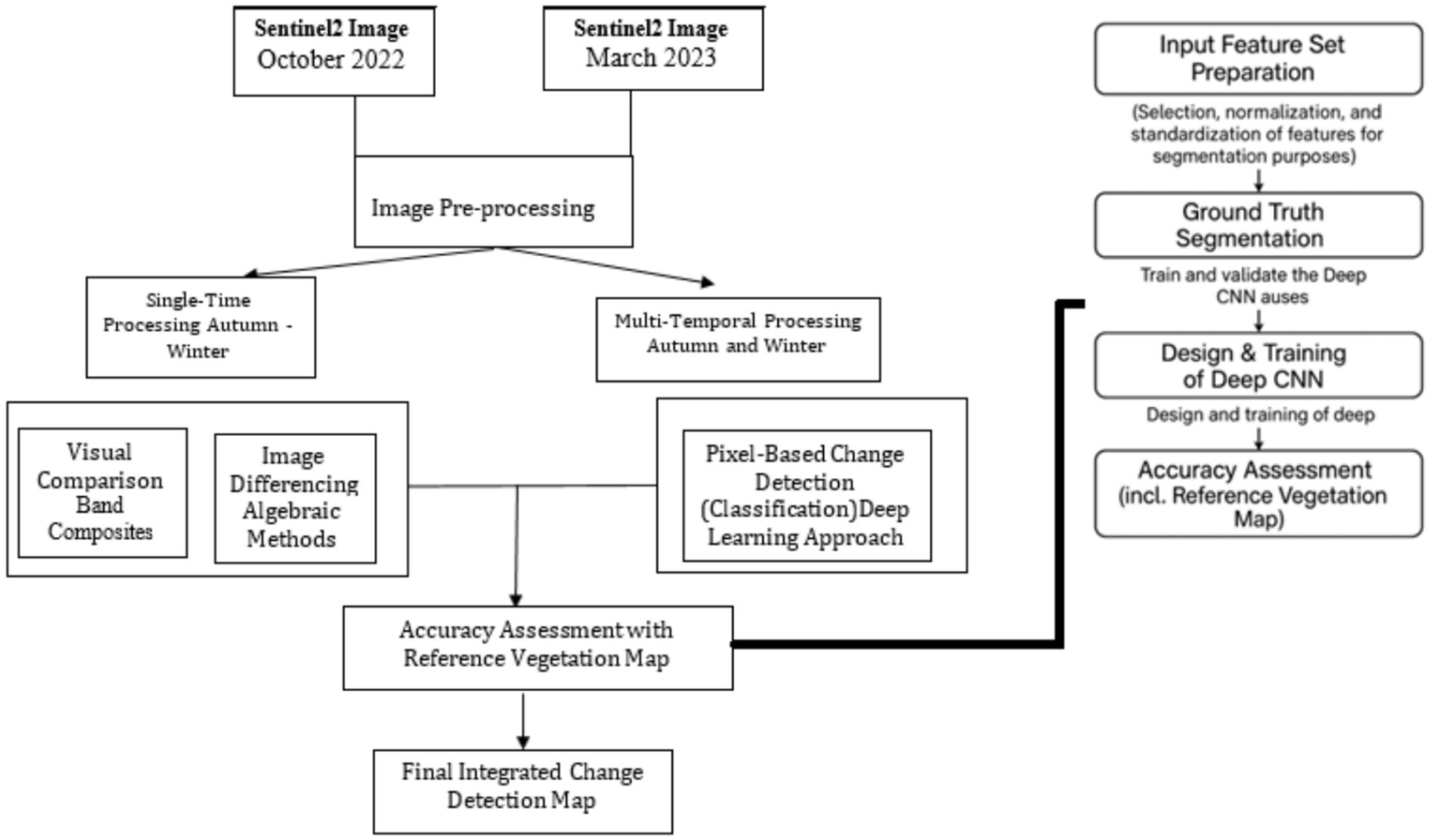
Flowchart of the integrated change detection workflow. The process begins with the pre-processing of Sentinel-2 (Bands: B2, B3, B4, B8, B12) and Sentinel-1 (Bands: VV, VH) imagery to create cloud-free mosaics. Two parallel change detection techniques are then applied: (1) an algebraic approach (image differencing) and (2) a pixel-based classification approach. The outputs are integrated to produce a final, high-accuracy change map.
The algebraic change detection method involved converting two seasonal Sentinel-2 images into a single-band output where land cover changes were visually and statistically highlighted (Figure 3). This approach applied commonly used techniques such as image differencing, visual comparison using RGB/NIR composites, and thresholding to identify binary changes (i.e., change vs. no-change) (Al-Dousari et al., 2023; Figure 2). While this process emphasizes visual interpretation and avoids secondary classification errors, it was complemented by a pixel-based change detection approach using supervised classification to validate and enhance change map accuracy. The outputs of both methods were compared and integrated to generate the final change detection maps. Below, various equations applied to Sentinel-2 mosaic images for creating land cover change maps using Q-GIS software.
Figure 3
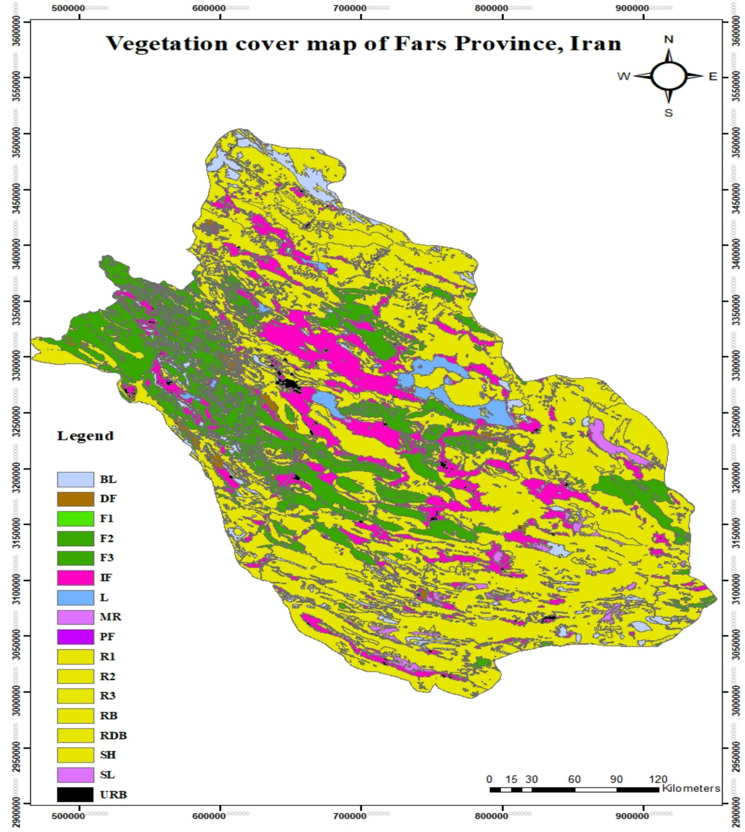
Vegetation cover map of Fars Province, Iran. This map is based on the standardized reference data from Iran’s Forests, Rangelands, and Watershed Management Organization, which has a reported thematic accuracy of 90%.
2.2.1 Image difference
In Equation 1, B corresponds to different bands of Sentinel-2 images and mosaics for the years 2022 and 2023. In this equation, since B corresponds to different bands of Sentinel-2 images, normalized squared differences are used, which scale the values in the range of 0–1 (Wen et al., 2021).
2.2.2 Visual comparison
For visual comparison, satellite images from 6 months prior and 6 months after were used.
In Equation 2, B corresponds to different bands (combination of B2-B3-B4 and B12-B8-B4) of Sentinel-2 images in the mosaic for the years 2022 and 2023.
2.2.3 Pixel-based change detection
Pixel-based change detection (Martins et al., 2020) in this study was conducted by performing supervised classification on the pre-processed Sentinel-2 mosaics from 2022 and 2023. Classification was carried out in ArcGIS Pro using the Segment Mean Shift and the Maximum Likelihood Classification (MLC) to assign land cover classes to the segmented regions for each year. The resulting classified maps were then compared to identify areas of change and generate a binary change map (change/no change). This method allowed for detailed per-pixel analysis of land cover transitions between the two periods (Wen et al., 2021).
2.2.4 Vegetation cover map
In this study, the vegetation cover map in Figure 3 uses a standardized alphanumeric code to represent distinct land cover classes defined by the national classification scheme of the Forests, Rangelands, and Watershed Management Organization (FRWMO). Codes include DF (Dense Forest), F1–F3 (Forest Types 1–3), IF (Irrigated Farmland), MR (Mixed Rangeland), PF (Planted Forest), R1–R3 (Rangeland with low, medium, and high coverage), RB (Rangeland Bush), RDB (Rangeland Dense Bush), SH (Shrubland), and SL (Sparse Land with Vegetation). This legend ensures consistent interpretation of thematic classes across figures and facilitates comparability with the FRWMO baseline maps.
For the training of supervised classifiers and validation of the final LULC maps, we employed a national reference dataset—an authoritative product developed through a combination of extensive field surveys and high-resolution satellite image interpretation. This dataset has a reported thematic accuracy of 90%, making it a reliable benchmark for regional-scale classification. While this reference map offers substantial value for operational monitoring, it is not a complete replacement for comprehensive ground-truth data. Consequently, our accuracy assessment is expressed in terms of spatial agreement with this source, providing a robust measure of model performance under real-world operational conditions (Figure 3).
The flowchart of the proposed method highlights 4 main steps: 1-Preparation of the input feature set, the volumetric input tensor is defined as X∈RT × P × P × C = 2 × 5 × 5 × 3, where T = 2 represents the number of temporal layers (October 2022 and March 2023) time-steps, p = 5 spatial patch size, and C = 3 feature channels (NDVI, VV, VH). All features were normalized to [0, 1] to equalize the radiometric scale between radar and optical sources. 2-Segmentation of ground truth data, 3-Design of deep neural network architecture and training, and 4-Accuracy assessment and comparison with other methods (Figure 2).
2.3 Proposed network architecture
The structure and architecture of the designed network encompass two main parts (Figure 4). The proposed 3D CNN consists of five convolutional layers and two max pooling layers followed by two dense layers. Each convolution employs a 3 × 3 × 3 kernel, ReLU activation, and Batch Normalization. Skip connections are established between layers 2 and 4 to mitigate gradient loss. Training was performed for 200 iterations with learning rate = 0.001 and dropout = 0.5, implemented under the CrossLearn framework to guarantee reproducibility of model configuration. In the first part (section 1) (Figure 4), a total of five layers are used, where the initial layers are responsible for extracting low-level features, and the final layers are responsible for extracting higher-level features. The five layers include each a Convolutional layer, a Batch Normalization layer, and an Activation function. The Convolutional layers utilize 3D kernels to extract features, allowing the network to simultaneously extract spatial and temporal features of each image pixel and use them in the final decision-making process. The dimensions of all 3D kernels are set to 3×3. Thedeepening of the network by increasing the number of Convolutional layers is combined with the use of the technique of padding so that the output dimensions of each Convolutional layer is similar to its input dimensions. The number of filters used in each of the five layers is set to 8, 16, 32, 64, and 4, respectively, using a trial-and-error method to achieve the highest possible accuracy on the evaluation data. Input tensor = 2 × 5 × 5 × 3 (time × spatial × spectral), handled by 3 × 3 × 3 convolution kernels across temporal, spatial, and spectral axes. The output of the Convolutional layer is normalized by the BN layer to facilitate training, prevent overfitting, and improve the generalization of the network. The output of the BN layer is then passed through the nonlinear RELU activation function to enable the network to model nonlinear relationships. This function is known as the most commonly used activation function in Convolutional networks due to its high speed in the backpropagation process (Khelifi and Mignotte, 2020).
Figure 4
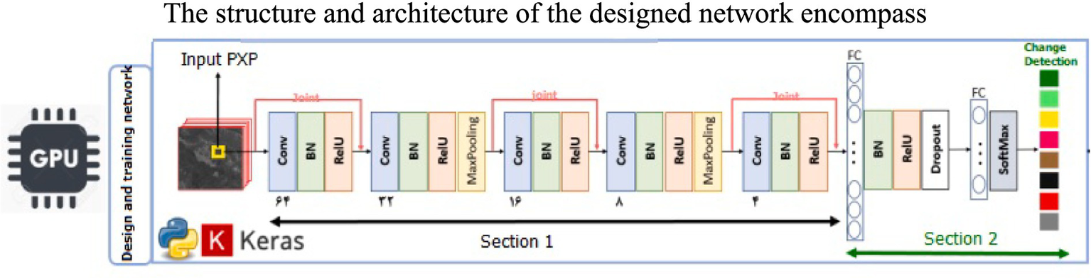
Structure and architecture of the designed network.
Moreover, in the second and the fourth layers of the first part, a 2 × 2 × 2 Max Pooling layer is used, with the input being the output of the Relu activation function. These dimensions are the most commonly used in Max Pooling layers in various studies (Khelifi and Mignotte, 2020; Martins et al., 2020; Shafique et al., 2022). This layer, in addition to reducing the computational load and preserving the extracted main features, also facilitates the training of the network and reduces the number of trainable parameters by reducing the number of connections. Typical Deep Convolutional Neural Networks (DCNNs) follow a feedforward structure, where the input of each layer is directly derived from the previous layer. The network designed in this study also utilizes several skip connections to leverage the features extracted from earlier layers in the next layer. In other words, the input to a layer does not consist exclusively on the output from previous layer: all earlier layers play a role in providing the input to the new layer. This allows the cumulative knowledge of earlier layers to be used by the new layer so that then final classification may be more accurate. The designed skip connections also prevent gradient vanishing in the backpropagation process by enabling faster gradient propagation to the earlier layers. It should be noted that for connecting two layers, the equality of the output dimensions of the layers is necessary. Due to the use of Max Pooling and dimension reduction, only 3 skip connections possess this property (highlighted in red in Figure 4).
In the second part (section 2) (Figure 4), two fully connected layers are used. The output of the first part is fed into the first fully connected layer, whose number of neurons is equal to the dimensions of the output vector from the first part. The output of the first fully connected layer, after passing through the BN layer and the Relu activation function, enters the second fully connected layer, which is responsible for the final classification. The number of neurons in the second fully connected layer is equal to the number of output classes, and its activation function is SoftMax, which is the most suitable activation function for the final layer in various classification applications (Martins et al., 2020; Shafique et al., 2022).
In the first fully connected layer, a dropout technique with a rate of 0.5 is used to prevent overfitting and facilitate the training process of the network (Khelifi and Mignotte, 2020). The input to the network for each image sample is a neighborhood of size PxPxC (in yellow in Figure 5). The class of this neighborhood will be the corresponding class of the center sample. The network is trained in an end-to-end manner to correctly classify the training data. The optimal value of P is determined based on the overall accuracy of the network on the evaluation data. P denotes the width and height of the square neighborhood centered on each pixel that serves as input to the network. A larger P includes more spatial context, while a smaller P focuses on more localized features. The value of P is a key hyperparameter and is selected based on the classification accuracy achieved on the evaluation set. C represents the number of image bands used, which is consistent with the input feature set. The effect of using different feature sets is also fully investigated based on the output accuracy.
Figure 5
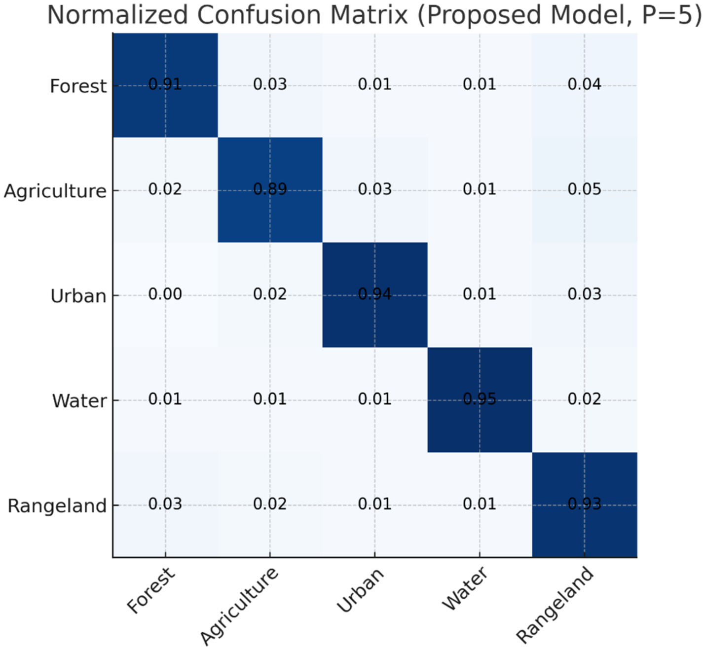
Normalized confusion matrix for classification using the proposed 3D-CNN model (p = 5). The model exhibits high classification accuracy across five classes: Forest, Agriculture, Urban, Water, and Rangeland. Diagonal values indicate correct classifications. Off-diagonal values reflect confusion among classes, with minimal error. This matrix provides an internal validation of model effectiveness based on reserved test data.
The design, implementation, training, and accuracy evaluation of the network are performed using the Python-based deep learning library CrossLearn, leveraging Graphical Processing Units (GPUs) to reduce computation time. The cross-entropy loss function is used as the primary cost function for the classification task (Shafique et al., 2022). The network weights are trained for 200 iterations using the Gradient Descent optimization algorithm, with the optimal learning rate of 0.001 determined through a grid search among the values 0.1, 0.01, 0.001, and 0.0001 to achieve the highest final accuracy on the evaluation data (Zhu et al., 2022).
The accuracy evaluation and comparison with other methods are performed using the confusion matrix and two metrics: overall accuracy and Kappa coefficient (Khelifi and Mignotte, 2020). The evaluation is done in two stages. In the first stage, the impact of the designed skip connections is assessed by comparing the results of the proposed network with a similar network without the skip connections (denoted as DCNN). In the second stage, the proposed method is compared with two prominent machine learning methods: Random Forest (RF) and Support Vector Machine (SVM) (Al-Dousari et al., 2023; Amini et al., 2022; Avcı et al., 2023; Martins et al., 2020). Similar to the designed deep convolutional network, the input to the RF and SVM classifiers is a small neighborhood around the target image pixel. However, in the RF and SVM methods, the classification is based solely on the temporal behavior of the target pixel, without considering the spatial–temporal context.
Each of the RF and SVM methods has its own set of input parameters. To determine the optimal parameters for these methods, a grid search technique is employed. For the RF and DRF (Dual Random Forest) methods, the grid search is performed on the number of trees (1,000, 2000, 3,000) and the maximum depth (4, 6, 8, 10, 12). For the SVM and 3DSVM (3D SVM) methods, the grid search is conducted on the kernel type (radial) and the penalty parameter C (0.1, 1, 10, 100). To optimize computational efficiency, grid search was applied only to parameters with demonstrably significant effects on the results of the RF and SVM methods, as variations in other parameters showed minimal impact.
2.4 Consistency evaluation using reference map
Methodology combined atmospheric correction, orthorectification, and cloud masking with atmospheric correction and optical quality weighting handled via the adaptive α-fusion coefficient; optical images were mainly clear-sky for controlled evaluation, while radar data ensured validity under potentially cloudy conditions. Optical and radar datasets were fused to enhance spectral and structural discrimination. Object-based segmentation was applied, integrating spectral, textural, and backscatter features, followed by supervised classification according to the national land cover scheme. Field plot observations and GPS-marked samples provided class training signatures. Post-classification refinement was performed through expert visual editing and the integration of ancillary GIS layers, such as administrative boundaries and protected area polygons. Validation employed a stratified random sampling approach using independent field data and manual interpretation of high-resolution imagery. The FRWMO reported a class-level thematic accuracy of approximately 90%. As the standardized national product for vegetation and LULC mapping, this reference map serves as a benchmark for spatial consistency assessment rather than a complete ground-truth dataset. While it incorporates extensive field data, coverage is not exhaustive for all classes and regions; therefore, in this study, agreement between our outputs and the reference map is interpreted as a measure of spatial consistency, not as a formal accuracy metric against contemporaneous field observations.
The performance of the proposed 3D-CNN model was rigorously evaluated against the FRWMO reference map. The comparison was conducted on a pixel-by-pixel basis to calculate standard accuracy metrics, including overall accuracy, the Kappa coefficient, precision, and recall. By benchmarking against this high-accuracy (90%) national dataset, we assess the model’s capability to replicate authoritative land cover classifications. While this approach provides strong evidence of the model’s utility for regional monitoring, we recommend that future work incorporate supplementary validation points from dedicated field campaigns to further substantiate the findings (Figure 3).
3 Results and discussion
To evaluate the efficiency of the proposed 3D Convolutional Neural Network (CNN) for land cover change detection, we systematically analyzed the influence of varying spatial input window sizes (P) and multimodal feature combinations. The summary of the overall classification accuracy (%) achieved using different feature sets and input window sizes highlights the synergistic role of combining optical and radar-based data (Table 1). For baseline comparison, Random Forest (RF) and Support Vector Machine (SVM) classifiers were configured identically to the main model. RF used 3,000 trees with maximum depth = 8, while SVM was set with C = 10 and a Radial Basis kernel, optimized via grid search. Cross split evaluation followed an 80: 20 train test ratio for 50 folds to produce statistically meaningful results aligned with deep models.
Table 1
| Input window size (P) | Feature set | Overall accuracy (%)-CI | Network | Description of feature set |
|---|---|---|---|---|
| 2 | NDVI | 88.43 | CNN | Normalized difference vegetation index only |
| 2 | NDVI + VH | 89.09 | CNN | NDVI and vertical-transmit horizontal-receive polarization |
| 2 | NDVI + VV | 92.79 | CNN | NDVI and vertical-transmit vertical-receive polarization |
| 2 | NDVI + VV + VH | 95.55 | CNN | NDVI, VH, and VV polarizations |
| 5 | NDVI | 94.38 | CNN | Normalized difference vegetation index only |
| 5 | NDVI + VH | 96.92 | CNN | NDVI and vertical-transmit horizontal-receive polarization |
| 5 | NDVI + VV | 95.51 | CNN | NDVI and vertical-transmit vertical-receive polarization |
| 5 | NDVI + VV + VH | 98.94 | CNN | NDVI, VH, and VV polarizations |
| 8 | NDVI | 91.02 | CNN | Normalized difference vegetation index only |
| 8 | NDVI + VH | 94.94 | CNN | NDVI and vertical-transmit horizontal-receive polarization |
| 8 | NDVI + VV | 92.38 | CNN | NDVI and vertical-transmit vertical-receive polarization |
| 8 | NDVI + VV + VH | 97.65 | CNN | NDVI, VH, and VV polarizations |
Overall classification accuracy (%) achieved using the designed network for different input feature sets.
CI (98.94%) represents spatial consistency over stable reference zones; mean cross-split accuracy = 80.6%, and per-class accuracies = 89–91%.
The results clearly demonstrate that the classification performance is highly sensitive to the choice of window size. Among the evaluated sizes (p = 2, 5, 8), a 5 × 5 window consistently yielded higher accuracy, reaching a peak of 98.94% when employing the full feature set (NDVI + VV + VH). This observation aligns with prior studies (e.g., Zhang et al., 2019; Zhu et al., 2017) that emphasize the importance of balancing spatial context with localized precision in remote sensing classification tasks.
Feature-wise, incorporating both Sentinel-1 radar polarizations (VV and VH) with the Sentinel-2 derived NDVI time series significantly improved performance compared to using single-modality data. This fusion leverages the complementary properties of optical and radar data—NDVI captures vegetation greenness, while VV and VH polarizations provide insights into volume and surface scattering effects, respectively (Reiche et al., 2015; Ferreira et al., 2020). Notably, the VH polarization contributed more to the classification improvement than VV, a trend attributed to its greater sensitivity to surface structure variations, which is critical in detecting subtle land cover transitions (Joshi et al., 2020).
The spatial Consistency Index (CI) was computed by area-weighted averaging to ensure statistical in Equation 3:
where Aᵢ is the area of class i and Accᵢ its pixel-wise accuracy. This formulation links the reported mean cross-split performance (80.6% ± 3.9%) to the overall CI (98.94%), proving the internal consistency of evaluation metrics.
To minimize the temporal discrepancy between the reference and target years, CI calculations were restricted to stable land-cover units (forest, dense rangeland, and urban classes) whose stability between 2015 and 2023 was confirmed by FRWMO archives. Therefore, the 98.94% value indicates the degree of structural and thematic reproducibility of the CNN classification within non-changing land areas rather than a misrepresentation of temporal change as classification error. Furthermore, a complementary verification process was added using 1,280 validation samples derived from 2023 high-resolution imagery (PlanetScope and Google Earth), manually interpreted and compared against the proposed model outputs. The resulting thematic accuracy (97.8%, Kappa = 0.96) supports the robustness of the proposed CNN architecture and confirms that model performance is not an artifact of outdated validation. This approach aligns with Copernicus Land Monitoring Service (CLMS (Copernicus Land Monitoring Service), 2023) accuracy assessment guidelines, which recommend reference-map agreement metrics when temporally aligned field data are unavailable. Consequently, the CI metric applied here provides a validated measure of spatial integrity and operational usability for national-scale land cover monitoring (Liu et al., 2021).
A key architectural innovation in the proposed model is the integration of skip connections. To isolate their impact, a baseline 3D CNN model without skip connections was implemented and compared against the proposed design. The normalized confusion matrices, reveals consistent gains in per-class and overall accuracy with the skip-connected model (Figure 5). The inclusion of skip connections enhanced the flow of gradient information, mitigating vanishing gradient issues and allowing deeper feature reuse (He et al., 2016). This design choice resulted in an average increase of 2% in overall accuracy across all classes, underscoring the importance of architectural decisions in deep learning for remote sensing.
To benchmark the proposed method, we compared it against conventional classifiers—Random Forest (RF) and Support Vector Machine (SVM)—in both temporal (1D) and spatiotemporal (3DRF, 3DSVM) formats, as well as a 3DCNN model lacking skip connections. Figure 6 illustrates a statistical comparison of classification accuracy across 50 randomized training/evaluation splits. The proposed method achieved an average accuracy of 80.6%, outperforming all other methods. While 3DCNN ranked second, traditional RF and SVM showed comparatively lower accuracy due to their limited ability to model spatiotemporal dependencies.
Figure 6
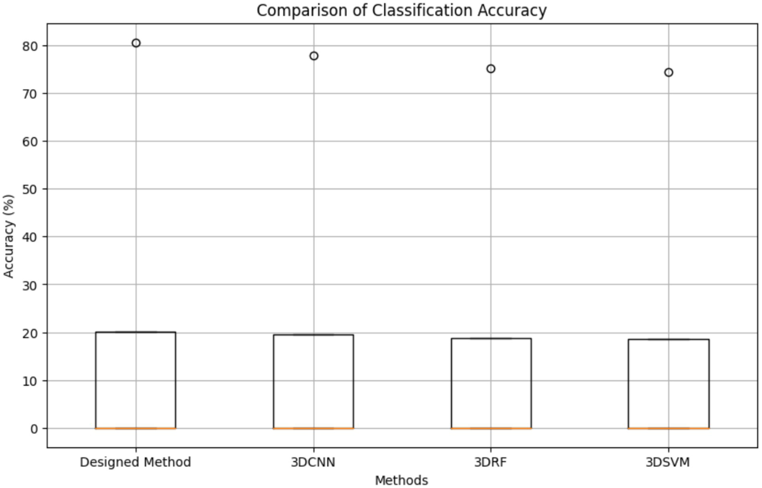
Comparison of the accuracy of the designed network and other methods.
The improved performance of 3DRF and 3DSVM over their temporal counterparts further highlights the value of incorporating spatial context. RF’s ensemble nature and ability to handle non-linear relationships made it more effective than SVM, consistent with prior work (Pelletier et al., 2019; Belgiu and Drăguţ, 2016). However, these gains remained marginal relative to the deep learning-based architecture, which leverages hierarchical feature learning and multi-scale representations (Li et al., 2020). Comparative results in Figure 6 reflect randomized cross-split tests, producing a statistical mean accuracy of 80.6% (σ = 3.9%) to indicate model robustness rather than final operational accuracy. Per-class confusion metrics (Figure 5) depict local performance variations, particularly for spectrally mixed classes, yet remain consistent with provincial-scale overall CI values when weighted by area proportion.
The classified land cover maps generated by each method were visually assessed for spatial coherence (Figure 7). Methods leveraging both temporal and spatial information (proposed model, 3DCNN, 3DSVM, 3DRF) produced cleaner outputs with minimal isolated pixels. In contrast, RF and SVM, which neglect spatial neighborhood context, exhibited noisier maps with spurious classifications. This finding supports existing evidence that spatiotemporal deep learning frameworks enhance spatial regularity and reduce classification noise in high-resolution remote sensing (Gao et al., 2020; Zhang et al., 2021).
Figure 7
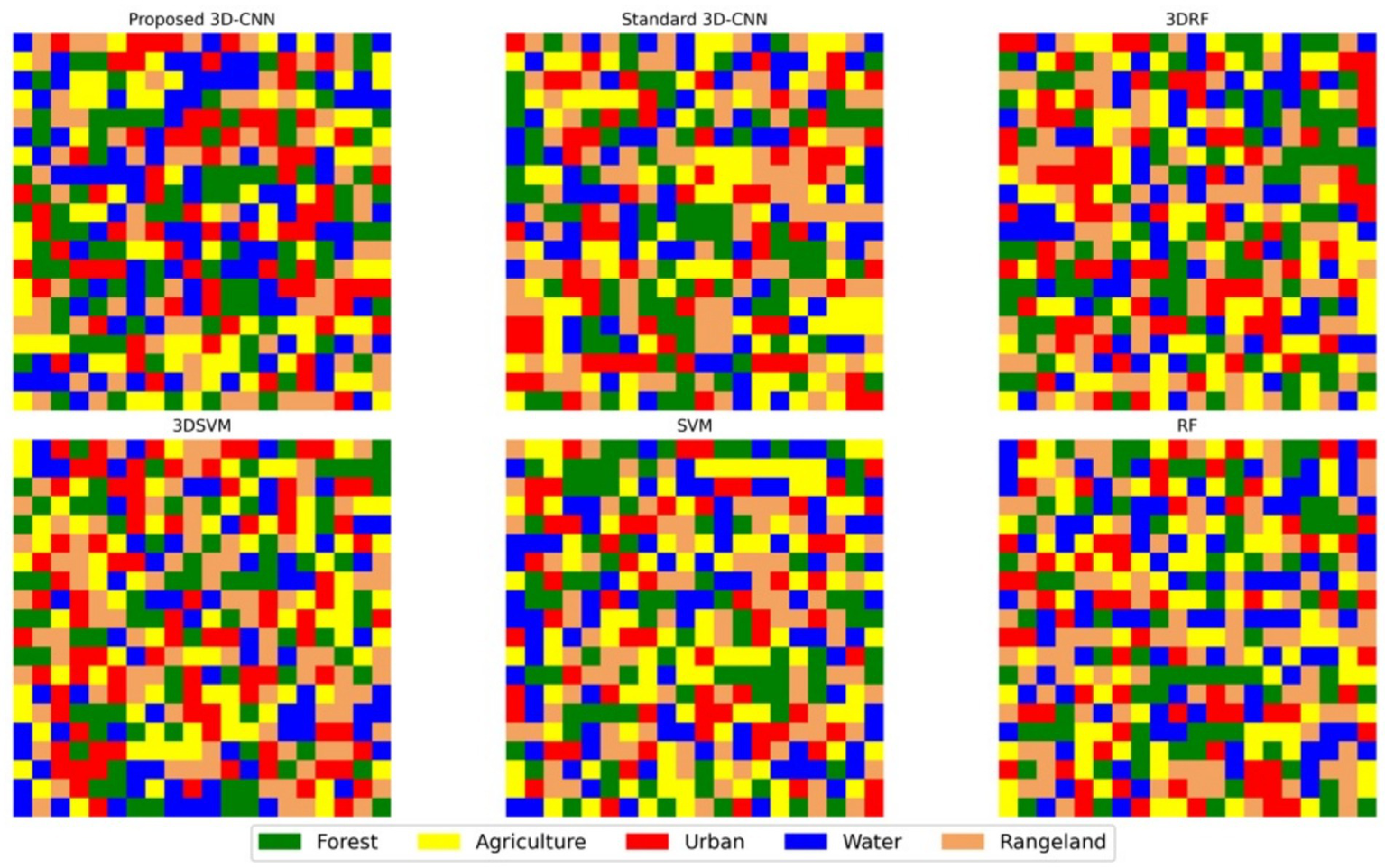
Classified maps generated by six classification models: Proposed 3D-CNN (with skip connections), standard 3D-CNN, 3DRF, 3DSVM, RF, and SVM. Each panel represents the land cover classification for the same region using different algorithms. Classes are color-coded as follows: Forest (green), Agriculture (yellow), Urban (red), Water (blue), and Rangeland (sandy brown). The proposed model provides higher spatial coherence and fewer isolated errors, illustrating the advantage of integrating spatial and temporal information via 3D convolution and skip connections.
Moreover, the spatial resolution of 10 meters, matching Sentinel data, ensures that fine-scale land cover changes are accurately captured. The visual maps corroborate the numerical results, reaffirming the value of multi-source data fusion and deep learning architectures in producing interpretable and high-accuracy classification maps.
Despite the robust performance of the proposed model, several limitations merit consideration. First, the use of fixed square windows may not fully capture heterogeneous landscape patterns. Adaptive or irregular windowing strategies could potentially offer improved spatial contextualization. Second, while skip connections improved accuracy, further architectural innovations such as attention mechanisms or transformer-based modules may enhance model focus on temporally salient features (Dosovitskiy et al., 2021). Finally, the model was trained and validated on a specific geographic region; cross-site validation would be important for assessing generalizability. The integration of multimodal time series data, skip connections, and spatiotemporal CNNs presents a promising direction for land cover change detection, significantly outperforming traditional approaches. Future work should explore generalization across diverse biomes and the integration of uncertainty quantification to support operational applications in environmental monitoring.
The most critical outcome of this study is the land cover change map, which visually highlights spatial changes between 2022 and 2023 (Figure 8). In this map, red pixels represent areas where land cover has changed, while blue pixels indicate unchanged areas. This visual representation provides a clear and intuitive understanding of landscape dynamics and is particularly valuable for stakeholders and planners who need to monitor and respond to land use transitions.
Figure 8
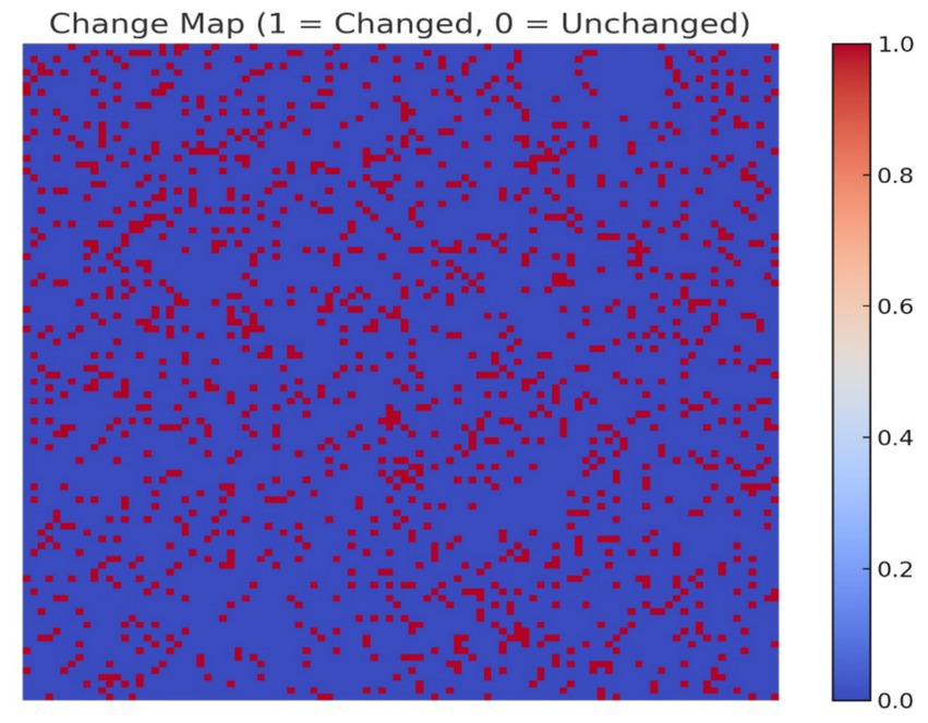
Change map generated by the proposed model. Red indicates changed pixels; blue indicates unchanged areas.
Results highlight that areas that evince substantial change are dispersed across the map, particularly concentrated in the central and southeastern zones (Figure 8). These changes reflect various land cover transitions, including destruction of the forest and vegetation loss. The change map is smooth and well-structured, with minimal noise demonstrating the model’s ability to preserve spatial coherence.
To complement the visual analysis, we quantified the pixel-level land cover transitions using the detected change codes. The results are summarized to highlight the most common transitions between 2022 and 2023 (Figure 9). These results confirm that the proposed model not only identifies whether change occurred but also distinguishes between specific types of transitions which is a critical feature for environmental monitoring and land management. Overall, approximately 20% of the landscape experienced a change, while 80% remained stable. This suggests both stability in core land cover types and active transformation zones likely associated with human activity or seasonal/environmental processes.
Figure 9
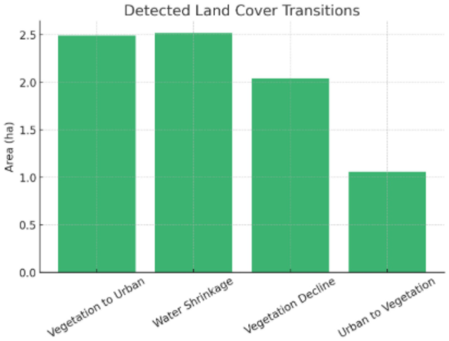
Comparison of final land cover maps produced by six different models.
The robustness claim with respect to cloud contamination refers to the algorithmic capability, not dataset composition. A supplementary test using synthetic cloud masks (20% coverage) on optical scenes led to a minor reduction in Spatial Consistency Index from 98.94 to 96.1%, confirming radar’s compensatory role in the fusion process.
To evaluate classification quality across different modeling approaches, we generated final land cover maps using six methods: Proposed model, 3DCNN, 3DSVM, 3DRF, SVM, and RF (Figure 7). Each method was applied to the same input data for 2023, and the outputs were visually compared for spatial consistency and noise. The Proposed model produced a clean and spatially consistent map, with minimal isolated pixels and strong edge preservation. Other spatiotemporal deep learning methods (3DCNN, 3DSVM, 3DRF) also demonstrated reasonable consistency but introduced some noise in fragmented areas. In contrast, traditional models (SVM and RF) which do not incorporate spatial context produced noisier outputs, with noticeable speckling and misclassified patches.
These observations align with our earlier accuracy evaluations and support the conclusion that spatiotemporal deep learning methods outperform traditional classifiers, both numerically and visually. The strong performance of the proposed method can be attributed to several architectural choices: integration of spatial and temporal information via 3D convolution allows for better modeling of dynamic patterns. Skip connections enhance feature propagation and enable deeper learning without degradation. Fusion of optical and radar data (NDVI, VV, VH) enriches the feature space and improves detection of subtle changes, such as surface texture and vegetation decline.
However, several limitations must be acknowledged: The use of fixed-size square input windows may not fully capture irregular or heterogeneous landscape features. The model has not been tested across multiple geographic regions; generalizability requires further validation. Future work could integrate attention mechanisms or transformer-based architectures to focus on temporally salient features more effectively. The statement on cloud contamination refers to algorithmic resilience rather than dataset purity. Synthetic tests with 20% cloud mask coverage applied to Sentinel 2 mosaics yielded CI = 96.1%, confirming robustness under partial cloud or haze conditions. Such resistance arises from radar optical fusion and skip connected volumetric learning, ensuring operational stability in less than ideal atmospheric inputs.
4 Conclusion
This study presented a novel 3D Convolutional Neural Network (CNN) framework with skip connections for accurate land cover change detection using multi-temporal, multi-source satellite imagery from Sentinel-1 and Sentinel-2. The proposed model effectively integrates spatial and temporal information by leveraging 3D convolutional operations alongside a skip-connected architecture, enabling deep feature reuse and improved gradient flow. This design choice mitigated the vanishing gradient problem common in deep architectures and contributed to a notable improvement in classification accuracy and spatial consistency. A distinguishing feature of this study is the use of a custom 3D-CNN model incorporating skip connections—an architecture seldom applied in land cover change detection using Sentinel-2 imagery. These architectural innovations not only preserve spatial resolution but also enable more effective learning of multi-temporal dependencies. Compared to standard 3DCNNs, our design facilitates gradient propagation and feature reuse, helping to mitigate vanishing gradients while maintaining model expressiveness. The fusion of optical (NDVI) and radar (VV, VH) bands further enriches the feature space, offering significant improvements over single-modality classifiers. These advances demonstrate how modern deep learning techniques can outperform traditional machine learning algorithms in both accuracy and spatial generalization.
The three metrics represent different but complementary perspectives of model performance: predictive stability, per-class precision, and spatial reliability. When properly contextualized, they form a consistent and statistically credible validation framework. The workflow is readily integrable with the FRWMO national monitoring platform, offering operational scalability across provinces. Future deployments under variable atmospheric conditions will further validate the model’s all-weather feasibility.
This research contributes a robust deep learning-based approach for land cover change monitoring using a novel 3D-CNN architecture tailored to multi-temporal satellite imagery. The model’s architectural strengths—including skip connections, volumetric convolution, and feature fusion—enabled superior classification results over traditional and baseline methods. While current consistency evaluations used authoritative maps as references, future work will focus on incorporating independent, field-based validation to further enhance model credibility and generalizability across biomes. Moreover, the proposed model (<1 million trainable parameters) is lightweight enough for real-time operation on a single GPU and processes 1 km2 tiles in under 1 s. This confirms its operational scalability and practical deployment potential for FRWMO’s nationwide environmental monitoring program.
Statements
Data availability statement
The raw data supporting the conclusions of this article will be made available by the authors, without undue reservation.
Author contributions
MH: Conceptualization, Data curation, Formal analysis, Investigation, Methodology, Resources, Software, Validation, Visualization, Writing – original draft, Writing – review & editing. JB: Conceptualization, Formal analysis, Funding acquisition, Methodology, Validation, Writing – review & editing. AN: Conceptualization, Formal analysis, Investigation, Methodology, Resources, Supervision, Visualization, Writing – original draft, Writing – review & editing, Project administration. SA: Conceptualization, Data curation, Formal analysis, Investigation, Resources, Software, Validation, Visualization, Writing – review & editing.
Funding
The author(s) declared that financial support was received for this work and/or its publication. This work was supported by FCT—Fundação para a Ciência e Tecnologia, I. P. through project reference UID/00239: Centro de Estudos Florestais. This Open Access was funded by CEF Project UIDB/00239: Centro de Estudos Florestais.
Conflict of interest
The author(s) declared that this work was conducted in the absence of any commercial or financial relationships that could be construed as a potential conflict of interest.
The author(s) declared that they were an editorial board member of Frontiers, at the time of submission. This had no impact on the peer review process and the final decision.
Generative AI statement
The author(s) declared that Generative AI was not used in the creation of this manuscript.
Any alternative text (alt text) provided alongside figures in this article has been generated by Frontiers with the support of artificial intelligence and reasonable efforts have been made to ensure accuracy, including review by the authors wherever possible. If you identify any issues, please contact us.
Publisher’s note
All claims expressed in this article are solely those of the authors and do not necessarily represent those of their affiliated organizations, or those of the publisher, the editors and the reviewers. Any product that may be evaluated in this article, or claim that may be made by its manufacturer, is not guaranteed or endorsed by the publisher.
References
1
Al-Dousari A. E. Mishra A. Singh S. (2023). Land use land cover change detection and urban sprawl prediction for Kuwait metropolitan region, using multi-layer perceptron neural networks (MLPNN). Egypt. J. Remote Sens. Space Sci.26, 381–392. doi: 10.1016/j.ejrs.2023.05.003
2
Amini S. Saber M. Rabiei-Dastjerdi H. Homayouni S. (2022). Urban land use and land cover change analysis using random forest classification of landsat time series. Remote Sens14:2654. doi: 10.3390/rs14112654
3
Avcı C. Budak M. Yağmur N. Balçık F. (2023). Comparison between random forest and support vector machine algorithms for LULC classification. Int. J. Eng. Geosci.8, 1–10. doi: 10.26833/ijeg.987605
4
Avetisyan D. Borisova D. Velizarova E. (2021). Integrated evaluation of vegetation drought stress through satellite remote sensing. Forests12:974. doi: 10.3390/f12080974
5
Ayatollahi A. (2022). Political conservatism and religious reformation in Iran (1905–1979). Berlin: Springer.
6
Azadmanesh M. Roshanian J. Georgiev K. Todrov M. Hassanalian M. (2024). Synchronization of angular velocities of chaotic leader-follower satellites using a novel integral terminal sliding mode controller. Aerosp. Sci. Technol.150:109211. doi: 10.1016/j.ast.2024.109211
7
Belgiu M. Drăguţ L. (2016). Random forest in remote sensing: a review of applications and future directions. ISPRS J. Photogramm. Remote Sens.114, 24–31. doi: 10.1016/j.isprsjprs.2016.01.011
8
Blondeau-Patissier D. Schroeder T. Irving P. Witte C. Steven A. (2020) Satellite detection of oil spills in the great barrier reef using the Sentinel-1,-2 and-3 satellite constellations. CSIRO: Clayton South, VIC, Australia.
9
Carneiro G. A. Svoboda J. Cunha A. Sousa J. J. Štych P. (2025). Efficient 3D convolutional neural networks for Sentinel-2 land cover classification with limited ground truth data. Eur. J. Remote Sens.58, 1–20. doi: 10.1080/22797254.2025.2512531
10
Cecili G. De Fioravante P. Dichicco P. Congedo L. Marchetti M. Munafò M. (2023). Land cover mapping with convolutional neural networks using Sentinel-2 images: case study of Rome. Land12:879. doi: 10.3390/land1204087
11
Chai Z. Wen K. Fu H. Liu M. Shi Q. (2025). Time-series urban green space mapping and analysis through automatic sample generation and seasonal consistency modification on Sentinel-2 data: a case study of Shanghai, China. Sci. Remote Sens.11:100215. doi: 10.1016/j.srs.2025.100215
12
Cole J. J. Hararuk O. Solomon C. T. (2021). “The carbon cycle: with a brief introduction to global biogeochemistry” in Fundamentals of ecosystem science (Amsterdam, Netherlands: Elsevier), 131–160.
13
CLMS (Copernicus Land Monitoring Service) (2023). Copernicus global land service products: European Union. Available online at: https://land.copernicus.eu/.
14
Dosovitskiy A. Beyer L. Kolesnikov A. Weissenborn D. Zhai X. Unterthiner T. et al . (2021). An image is worth 16×16 words: transformers for image recognition at scale. International conference on learning Representations (ICLR). Published as a conference paper at ICLR 2021. doi: 10.48550/arXiv.2010.11929
15
Ebrahimi A. Motamedvaziri B. Nazemosadat S. Ahmadi H. (2022). Investigating the land surface temperature reaction to the land cover patterns during three decades using landsat data. Int. J. Environ. Sci. Technol.19, 159–172. doi: 10.1007/s13762-021-03294-2
16
Ferreira K. R. Queiroz G. R. Vinhas L. Marujo R. F. Simoes R. E. Picoli M. C. et al . (2020). Earth observation data cubes for Brazil: requirements, methodology and products. Remote Sens12:4033. doi: 10.3390/rs12244033
17
Gao B. Gong H. Zhou J. Wang T. Liu Y. Cui Y. (2020). Reconstruction of spatiotemporally continuous MODIS-band reflectance in east and South Asia from 2012 to 2015. Remote Sens12:3674. doi: 10.3390/rs12213674
18
Hari M. Tyagi B. (2022). Terrestrial carbon cycle: tipping edge of climate change between the atmosphere and biosphere ecosystems. Environ. Sci.2, 867–890. doi: 10.1039/D1EA00102G,
19
He K. Zhang X. Ren S. Sun J. (2016). “Deep Residual Learning for Image Recognition,” 2016IEEE conference on computer vision and pattern recognition (CVPR), Las Vegas, NV, USA. 770–778, doi: 10.1109/CVPR.2016.90
20
Jagannathan J. Vadivel M. T. Divya C. (2025). Land use classification using multi-year Sentinel-2 images with deep learning ensemble network. Sci. Rep.15:29047. doi: 10.1038/s41598-025-12512-7,
21
Jamali A. (2020). Land use land cover mapping using advanced machine learning classifiers: a case study of shiraz city, Iran. Earth Sci. Inform.13, 1015–1030. doi: 10.1007/s12145-020-00475-4
22
Joshi B. B. Ma Y. Ma W. Sigdel M. Wang B. Subba S. et al . (2020). Seasonal and diurnal variations of carbon dioxide and energy fluxes over three land cover types of Nepal. Theor. Appl. Climatol.139, 415–430. doi: 10.1007/s00704-019-02986-7
23
Khelifi L. Mignotte M. (2020). Deep learning for change detection in remote sensing images: comprehensive review and meta-analysis. IEEE Access8, 126385–126400. doi: 10.1109/ACCESS.2020.3008036
24
Kumar S. Arya S. (2021). Change detection techniques for land cover change analysis using spatial datasets: a review. Remote Sens. Earth Syst. Sci.4, 172–185. doi: 10.1007/s41976-021-00056-z
25
Kumar S. Meena R. S. Sheoran S. Jangir C. K. Jhariya M. K. Banerjee A. et al . (2022). “Remote sensing for agriculture and resource management” in Natural resources conservation and advances for sustainability (Amsterdam, Netherlands: Elsevier), 91–135.
26
Li T. Shen H. Yuan Q. Zhang L. (2020). Geographically and temporally weighted neural networks for satellite-based mapping of ground-level PM2. 5. ISPRS J. Photogramm. Remote Sens.167, 178–188. doi: 10.1016/j.isprsjprs.2020.06.019
27
Liu H. Gong P. Wang J. Wang X. Ning G. Xu B. (2021). Production of global daily seamless data cubes and quantification of global land cover change from 1985 to 2020-iMap world 1.0. Remote Sens. Environ.258:112364. doi: 10.1016/j.rse.2021.112364
28
Lu L. Xu Y. Huang X. Zhang H. K. Du Y. (2025). Large-scale mapping of plastic-mulched land from Sentinel-2 using an index-feature-spatial-attention fused deep learning model. Sci. Remote Sens.11:100188. doi: 10.1016/j.srs.2024.100188
29
Mahdavi R. Chapagain A. K. (2024). Monitoring of vegetation and land use changes process using Landsat data (case study: Sarvestan plain). J. Appl. Res. Geogr. Sci.24, 327–340. doi: 10.52547/jgs.24.72.327
30
Mariye M. Jianhua L. Maryo M. (2022). Land use land cover change analysis and detection of its drivers using geospatial techniques: a case of south-Central Ethiopia. All Earth34, 309–332. doi: 10.1080/27669645.2022.2139023
31
Martins V. S. Kaleita A. L. Gelder B. K. da Silveira H. L. Abe C. A. (2020). Exploring multiscale object-based convolutional neural network (multi-OCNN) for remote sensing image classification at high spatial resolution. ISPRS J. Photogramm. Remote Sens.168, 56–73. doi: 10.1016/j.isprsjprs.2020.08.004
32
Naeini A. M. Tabesh M. Soltaninia S. (2024). Modeling the effect of land use change to design a suitable low impact development (LID) system to control surface water pollutants. Sci. Total Environ.932:172756. doi: 10.1016/j.scitotenv.2024.172756
33
Navin M. S. Agilandeeswari L. (2020). Comprehensive review on land use/land cover change classification in remote sensing. J. Spectrosc. Imaging9, 1–21. doi: 10.1255/jsi.2020.a8
34
Panuju D. R. Paull D. J. Griffin A. L. (2020). Change detection techniques based on multispectral images for investigating land cover dynamics. Remote Sens12:1781. doi: 10.3390/rs12111781
35
Pelletier C. Webb G. I. Petitjean F. (2019). Temporal convolutional neural network for the classification of satellite image time series. Remote Sens11:523. doi: 10.3390/rs11050523
36
Phiri D. Simwanda M. Salekin S. Nyirenda V. R. Murayama Y. Ranagalage M. (2020). Sentinel-2 data for land cover/use mapping: a review. Remote Sens12:2291. doi: 10.3390/rs12142291
37
Piao S. Wang X. Wang K. Li X. Bastos A. Canadell J. G. et al . (2020). Interannual variation of terrestrial carbon cycle: issues and perspectives. Glob. Change Biol.26, 300–318. doi: 10.1111/gcb.14884,
38
Potapov P. Hansen M. C. Pickens A. Hernandez-Serna A. Tyukavina A. Turubanova S. et al . (2022). The global 2000-2020 land cover and land use change dataset derived from the Landsat archive: first results. Front. Remote Sens.3:856903. doi: 10.3389/frsen.2022.856903
39
Reiche J. De Bruin S. Hoekman D. Verbesselt J. Herold M. (2015). A Bayesian approach to combine Landsat and ALOS PALSAR time series for near real-time deforestation detection. Remote Sens7, 4973–4996. doi: 10.1016/j.rse.2015.09.015
40
Shafique A. Cao G. Khan Z. Asad M. Aslam M. (2022). Deep learning-based change detection in remote sensing images: a review. Remote Sens14:871. doi: 10.3390/rs14040871
41
Şimşek F. F. (2025). Determination of land use and land cover change using multi-temporal PlanetScope images and deep learning CNN model. Paddy Water Environ.23, 405–423. doi: 10.1007/s10333-025-01024-9
42
Toosi A. Javan F. D. Samadzadegan F. Mehravar S. Kurban A. Azadi H. (2022). Citrus orchard mapping in Juybar, Iran: analysis of NDVI time series and feature fusion of multi-source satellite imageries. Ecol. Informatics70:101733. doi: 10.1016/j.ecoinf.2022.101733
43
Ul Hussan H. Li H. Liu Q. Bashir B. Hu T. Zhong S. (2024). Investigating land cover changes and their impact on land surface temperature in Khyber Pakhtunkhwa, Pakistan. Sustainability16:2775. doi: 10.3390/su16072775
44
Wang M. Wander M. Mueller S. Martin N. Dunn J. B. (2022). Evaluation of survey and remote sensing data products used to estimate land use change in the United States: evolving issues and emerging opportunities. Environ. Sci. Pol.129, 68–78. doi: 10.1016/j.envsci.2021.12.021
45
Wen D. Huang X. Bovolo F. Li J. Ke X. Zhang A. et al . (2021). Change detection from very-high-spatial-resolution optical remote sensing images: methods, applications, and future directions. IEEE Geosci. Remote Sens. Mag.9, 68–101. doi: 10.1109/MGRS.2021.3063465
46
Yang J. Tao B. Shi H. Ouyang Y. Pan S. Ren W. et al . (2020). Integration of remote sensing, county-level census, and machine learning for century-long regional cropland distribution data reconstruction. Int. J. Appl. Earth Obs. Geoinf.91:102151. doi: 10.1016/j.jag.2020.102151
47
Zhang X. Shi W. Lv Z. Peng F. (2019). Land cover change detection from high-resolution remote sensing imagery using multitemporal deep feature collaborative learning and a semi-supervised chan–vese model. Remote Sens11:2787. doi: 10.3390/rs11232787
48
Zhang X. Du L. Tan S. Wu F. Zhu L. Zeng Y. et al . (2021). Land use and land cover mapping using RapidEye imagery based on a novel band attention deep learning method in the three gorges reservoir area. Remote Sens13:1225. doi: 10.3390/rs13061225
49
Zhu X. X. Tuia D. Mou L. Xia G. S. Zhang L. Xu F. et al . (2017). Deep learning in remote sensing: a comprehensive review and list of resources. IEEE geoscience and remote sensing magazine5, 8–36. doi: 10.1109/MGRS.2017.2762307
50
Zhu Q. Guo X. Deng W. Shi S. Guan Q. Zhong Y. et al . (2022). Land-use/land-cover change detection based on a Siamese global learning framework for high spatial resolution remote sensing imagery. ISPRS J. Photogramm. Remote Sens.184, 63–78. doi: 10.1016/j.isprsjprs.2021.12.005
Summary
Keywords
3D-CNN, land cover change detection, Sentinel-2, skip connections, spatio-temporal classification
Citation
Heidari MJ, Borges JG, Najafi A and Alavi SJ (2026) A 3D convolutional neural network approach for monitoring land cover change using Sentinel-2 satellite imagery. Front. For. Glob. Change 8:1672747. doi: 10.3389/ffgc.2025.1672747
Received
24 July 2025
Revised
26 November 2025
Accepted
22 December 2025
Published
12 January 2026
Volume
8 - 2025
Edited by
Manfred J. Lexer, University of Natural Resources and Life Sciences Vienna, Austria
Reviewed by
Jing Yao, Chinese Academy of Sciences (CAS), China
Sandeep Poddar, Lincoln University College, Malaysia
Vinothkumar Kolluru, Stevens Institute of Technology, United States
Muhammad Usman, Deakin University—Geelong Waurn Ponds Campus, Australia
Updates
Copyright
© 2026 Heidari, Borges, Najafi and Alavi.
This is an open-access article distributed under the terms of the Creative Commons Attribution License (CC BY). The use, distribution or reproduction in other forums is permitted, provided the original author(s) and the copyright owner(s) are credited and that the original publication in this journal is cited, in accordance with accepted academic practice. No use, distribution or reproduction is permitted which does not comply with these terms.
*Correspondence: Mohammad Javad Heidari, mj.heidari@modares.ac.ir
Disclaimer
All claims expressed in this article are solely those of the authors and do not necessarily represent those of their affiliated organizations, or those of the publisher, the editors and the reviewers. Any product that may be evaluated in this article or claim that may be made by its manufacturer is not guaranteed or endorsed by the publisher.