Abstract
Understanding ecosystem function and dynamics is essential for crafting effective, long-term forest management strategies. Our study integrates chronosequence data, ecosystem modeling using Biome-BGCMuSo, and eddy covariance flux tower measurements to test the hypothesis that Net Ecosystem Productivity (NEP) reaches its maximum at a similar relative age across different forest types. We focused on contrasting biomes consisting of Northern Hardwoods, Douglas Fir, Jack Pine, Black Spruce and Southeastern hardwoods. Our results indicate broadly consistent NEP maximization across forest systems examined, with ecosystem modeling producing peak NEP at a relative stand age (ratio of stand age to site-specific longevity) of 0.24–0.39 and a transition to near-zero NEP between 0.46–0.86. This pattern aligns with Odum's conceptual model of ecosystem development, reflecting shifts in photosynthetic gains and respiratory losses as stands mature. Analysis combining chronosequence observations, process-based ecosystem model outputs, and eddy covariance measurements shows that NEP peaks at similar relative ages across forest types, a pattern that cannot be identified using a single approach in isolation. Sensitivity analyses under future climate change scenarios suggest that these patterns are robust to the tested range of environmental conditions. By synthesizing empirical data and process-based modeling, this analysis addresses limitations of traditional chronosequence studies, enhancing our ability to project net carbon sequestration across the complete lifespan of a stand. Our research provides model based quantitative evidence consistent with established ecological theories of forest carbon dynamics and contributes to the debate on forest carbon permanence and trade-offs in near-term climate mitigation strategies, such as harvest deferrals and stand re-establishment.
1 Introduction
Net ecosystem productivity (NEP), the balance between gross primary production (GPP) and ecosystem respiration (RE), determines annual carbon sequestration in forests and is influenced by environmental factors including solar radiation, air temperature, nutrients, water and structural characteristics such as stand age, species composition, tree height, leaf area index, and canopy density that change during stand development. Although environmental controls influence NEP, stand age consistently emerged among the predictors of spatial and temporal variation in NEP, because it reflects integrated changes in structure and function that collectively regulate ecosystem carbon balance (Besnard et al., 2018; Noormets et al., 2007).
During the initial years of stand development, either after a new establishment or a stand from regeneration after disturbance, the losses due to RA (autotrophic root respiration) and RH (soil organic matter decomposition) exceed the carbon sequestration resulting in forest ecosystems typically functioning as net carbon emission sources. The duration of this phase varies based on growth rates, site conditions, climate variables, and post-disturbance effects. Rapidly growing forests then transition to carbon sinks within approximately 10-20 years as increasing leaf area and biomass accumulation enhance carbon uptake and eventually surpasses carbon losses from respiration and decomposition. NEP reaches its maximum at an intermediate stand age, after which age-related declines in net primary production (NPP) occur due to reduced nutrient availability, increased mortality (Ryan, 1991; Hartmann and Trumbore, 2016), changes in stomatal conductance, and decreases in photosynthetic efficiency, which shift the balance between carbon uptake and respiratory losses (Bond-Lamberty et al., 2004; Gower et al., 1996; Tang et al., 2014), so that old-growth forests frequently function as a minor carbon sink, or remain carbon neutral, or even become a net emissions source, depending on various factors such as climate, disturbance history, and species composition (Chang et al., 2020; He et al., 2012).
The age-dependent carbon trajectory has its conceptual basis in the Odum (1969) succession model, which predicted changes in ecosystem energy flow and nutrient cycling with stand development. Odum's framework, supported by empirical work from Kira and Shidei (1967), posits that old-growth forests reach a near steady-state where additional carbon accumulation is minimal and largely balanced by mortality and decay (Gough et al., 2008). Several chronosequence studies are consistent with this pattern; for example, boreal black spruce stands in central Manitoba exhibit peak sink strength between 11 and 36 years before declining toward zero by approximately 130 years (Litvak et al., 2003). Similar age-related NEP patterns are observed in post-harvest boreal jack pine forests (Zha et al., 2009) and in white pine forests where NEP peaks around 19 years before diminishing in older stands (Peichl et al., 2010).
However, despite broad support for age-related declines in NEP, multiple studies challenge the assumption that old-growth forests are carbon neutral or near zero. Observational evidence from AmeriFlux and long-term eddy-covariance records shows that some mature forests maintain positive NEP for extended periods (Desai et al., 2005; Tan et al., 2011; Zhou et al., 2011). Syntheses of global flux datasets further indicate that old-growth forests can continue to sequester carbon (Luyssaert et al., 2008), and additional case studies from temperate and montane ecosystems demonstrate that mature stands may remain carbon sinks through increases in aboveground biomass, particularly in large-diameter trees (Luo et al., 2007; Carey et al., 2001; Noguchi et al., 2022).
Despite extensive empirical work on age-related NEP patterns, most existing evidence remains methodologically fragmented, limiting the ability to evaluate carbon flux trajectories across stand age and across forest types. Empirical studies rely exclusively on flux towers, biometric chronosequences, or site-level inventories, each of which captures only part of the stand development continuum and cannot fully isolate the effect of stand age from disturbance legacies, rising atmospheric CO2, regional climate variability, and nitrogen deposition (Goulden et al., 1996; Amiro et al., 2010). Long-term eddy covariance observations that span multiple developmental stages within unmanaged forests remain limited, while chronosequence studies infer temporal patterns by comparing sites of different ages, constraining the extent to which their results can be generalized across biomes. Moreover, because forest maturity occurs at different absolute ages across species and biomes, empirical studies cannot readily generalize the relationship between stand development and ecosystem productivity beyond their specific site context (Tang et al., 2009; Saiz et al., 2006; Tedeschi et al., 2006). Although process-based ecosystem models have been applied to forest carbon dynamics (Peichl et al., 2023), fewer studies have explicitly combined them with chronosequence and flux observations to evaluate NEP trajectories across contrasting forest systems.
Process-based ecosystem models provide a means to address these empirical limitations by simulating carbon fluxes under consistent physiological and environmental assumptions (Fuller et al., 2025). This allows stand-age effects to be evaluated independently of disturbance legacies and background environmental variability (rising CO2 and regional climate variability) that cannot be separated cleanly using observational datasets (Pregitzer and Euskirchen, 2004; Janssens et al., 2010).
In this study, we use the process-based ecosystem model Biome-BGCMuSo (Hidy et al., 2012, 2016, 2022), particularly suited to this problem because it represents canopy development, carbon allocation, respiration, turnover, and empirically formulated mortality interacting within a mechanistic modeling framework as stand structure evolves over time. In our framework, the model is driven by long-term climate records to simulate carbon flux dynamics across the full lifespan of each forest type, including developmental stages that are sparsely represented in chronosequence observations. Importantly, Biome-BGCMuSo does not impose a direct productivity or NEP function with respect to age. Instead, stand development patterns in NEP emerge implicitly from climate-driven changes in vegetation and soil carbon, nitrogen state variables that govern biomass accumulation through prescribed species ecophysiological traits and turnover dynamics regulated by the mortality formulation (details are provided in Section 2.2). It further provides a controlled setting to evaluate the sensitivity of NEP age relationships to projected changes in atmospheric CO2 and nitrogen deposition, a dimension that empirical datasets cannot capture and that has received limited attention in mechanistic studies (Canadell and Raupach, 2008; Chapin et al., 2006).
In this manuscript, we estimate the relative stand age of diverse forest ecosystems at which the productivity is maximized and determine the NEP variation through stand development. Our approach involves using chronosequence data and ecological modeling for different forest species to characterize temporal patterns of NEP as forests mature. Specifically, we conduct the following analyses to project peak NEP for different forest types in North America:
-
Find chronosequence sites and perform ecosystem model simulations for the forests in Northwestern and central America region to project patterns of NEP and cumulative NEP across the stand age gradient.
-
Estimate the relative stand age at which the NEP is maximized throughout the life of a stand.
-
Validate the optimal stand age theory for Southeastern US forests using theoretical relative stand age for maximum NEP.
-
Conduct sensitivity analysis of NEP to future atmospheric CO2 concentrations and N deposition rates consistent with projected future climate changes and socioeconomic developments.
We hypothesize that forest ecosystems reach maximum NEP at a similar relative stand age, defined as the ratio of stand age to species-specific longevity, across contrasting forest types. We further hypothesize that stands beyond maturity, as defined relative to species-specific longevity, tend toward carbon neutrality when evaluated using NEP. These hypotheses are evaluated within the broader conceptual framework of ecosystem development proposed by (Odum 1969). Additionally, we propose that under ideal conditions, the relative stand age for maximizing NEP would not substantially vary for different forest ecosystems, though disturbance or other external meteorological and environmental factors, such as atmospheric CO2, drought, and extreme climate events, could result in variations in the relative stand ages of peak NEP.
A key distinction of this analysis is the evaluation of NEP trajectories as a function of relative stand age within a common mechanistic framework, enabling direct comparison of peak timing and trajectory shape across contrasting forest types. By integrating empirical constraints with process-based modeling, we assess the consistency of NEP patterns, the timing of peak productivity, and late-successional NEP trends while explicitly accounting for species-specific longevity. These findings inform interpretation of forest carbon permanence and tradeoffs among near-term climate mitigation strategies in forestry, including harvest deferrals and stand re-establishment, without assuming uniform responses across ecosystems or management contexts.
2 Materials and methods
NEP data used in this study are compiled for forest chronosequences in North America containing different stand ages to capture the average lifespan of the dominant tree species. This analysis includes chronosequences containing critical stages in ecosystem development for each ecosystem that provides better experimental control than an unmatched collection of ad hoc sites. Estimates for the NEP were calculated using two approaches: the biometric method (B), which estimates NEP as the difference between net primary production (NPP) and heterotrophic respiration (RH) based on biomass and soil measurements, and the eddy covariance method (EC), which directly measures net carbon exchange between the ecosystem and the atmosphere using micrometeorological techniques. The choice of method varied by site, depending on data availability (see Supplementary material).
To select appropriate chronosequences for analysis, certain criteria were applied. These criteria included:
-
The chronosequence needed to consist of at least three stands from unmanaged sites of varying ages, originating from regeneration following both natural and anthropogenic disturbances.
-
The oldest stands within the chronosequence had to reach over 50% of the average lifespan of the dominant tree species.
-
NEP measurements for old-growth stands had to be conducted for more than one year or using multiple approaches. This last criterion is crucial due to the significant year-to-year variation in NEP.
Following these criteria, we identified five forest types with robust chronosequences, which encompass both boreal and temperate forests. Chronosequence datasets from studies such as Krishnan et al. (2009), Wharton et al. (2012), Dunn et al. (2007), and Zha et al. (2009) provided site-level NEP observations across a range of stand ages that met these conditions. A summary of the characteristics of each site is presented in Table 1 (additional details are available in the Supplementary material). Specifically, the sites JP-S, BS-Q, and DF-P have experienced disturbances from both wildfire and harvest, while NH-W has undergone disturbances from wind and harvest, and BS-M has been impacted solely by wildfire. The chronosequence data included in our study originated after these disturbances, providing a critical basis for understanding forest recovery and ecosystem dynamics.
Table 1
| Species | Location | Stand age & technique | Code | Longevity* | Latin name |
|---|---|---|---|---|---|
| Black spruce | Manitoba, Canada | †0,5,14,22,39,73,154 ‡1,5,14,22,39,73,146–155 | BS-M | 250-300 | Picea mariana |
| Jack pine | Saskatchewan, Canada | †0, 5, 10, 29, 79 ‡2, 3, 7–11, 29-31, 86–93 | JP-S | 150–200 | Pinus banksiana |
| Black spruce | Quebec, Canada | †2–10,33–35, †101–107 | BS-Q | 250–300 | Picea mariana |
| N.hardwoodsa | Wisconsin, USA | †7, 70–76, †352–356 | NH-W | 300–400 | Acer saccharum |
| Douglas fir | PNWb, Canada & USA | †1–6, 14–18 †9–56, 450–460 | DF-P | 500–1,000 | Pseudotsuga menziesii |
Summary of basic chronosequence characteristics.
*General longevity (years) (Burns and Honkala, 1990).
‡Biometric method (NPP – RH), †Eddy Covariance method.
aNorthern hardwoods,bPacific Northwest.
We employed a relative stand age metric to integrate and analyze both the chronosequence and modeled NEP datasets. Initial evaluation of the chronosequence data revealed notable gaps, particularly for intermediate stand ages across certain forest types. To supplement these limitations and enable a comprehensive assessment of NEP dynamics across stand development stages, we utilized the non-spatial version of the process-based ecosystem model Biome-BGCMuSo.
To estimate relative stand age, we first reviewed species-specific forest information from published literature and forest handbooks (Burns and Honkala, 1990) and established generic longevity ranges for the dominant tree species (Table 1). For each species, we calculated the midpoint of the reported minimum and maximum lifespan values as the baseline longevity estimate. To incorporate uncertainty, we applied a ±10% window around the midpoint. This relatively narrow range was selected because the chronosequence sites used in this study are geographically concentrated, with limited variation in soil, climate, and other ecological drivers that typically influence mortality and species longevity. We validated the longevity estimates by cross-referencing published site-specific information for the chronosequence data sites (Supplementary Table 1) to confirm the presence of old-growth stands reaching the estimated ages. Initially, we calculated a baseline longevity estimate as the midpoint of the published minimum and maximum species-specific lifespans and defined an uncertainty window of ±10% around this baseline. Where site-specific maximum observed stand ages fell outside this initial window, we incrementally adjusted the baseline longevity estimate by ±20%, ±30%, or higher as necessary, maintaining a constant ±10% uncertainty range, until the observed site-specific values were incorporated within the window. This iterative adjustment ensured that longevity assumptions accurately reflected both general species traits and empirical site-specific observations while consistently accounting for ecological variability. The relative stand age was calculated as:
This formulation enabled consistent comparison of NEP dynamics across forest types differing in absolute lifespan.
While the chronosequence data provided valuable insights, significant gaps existed in the intermediate stand development stages, particularly between relative stand ages of 0.25 and 0.45. To address these gaps and to simulate NEP across the full spectrum of forest development, we employed ecosystem process model Biome-BGCMuSo simulations. Biome-BGCMuSo and its previous versions have been widely used to simulate carbon fluxes and ecosystem productivity across stand and regional scales (Merganičová et al., 2005; Merganičová and Merganič, 2014; Ostrogović Sever et al., 2017, 2021).
Integrating Biome-BGCMuSo model simulations with chronosequence observations allowed us to validate NEP trends across forest developmental stages and test the hypothesis that different forest types achieve peak NEP at similar relative stand ages. The simulated NEP trajectories complemented empirical data, enabling projection of NEP trends through early development, peak productivity, and old-growth stages across the studied biomes.
To ensure objective validation of model outputs, we applied the two-sample Kolmogorov-Smirnov (KS) test (Goodbody et al., 2020; Olea and Pawlowsky-Glahn, 2009) to compare distributions of modeled and observed chronosequence NEP values across stand ages. For this analysis, we refined the chronosequence data to focus on the core stand development process by excluding initial negative NEP values typically associated with post-disturbance recovery, allowing for a more direct comparison of stand age effects on NEP dynamics. This refinement isolated stand development trends from complex disturbance-related influences, such as initial carbon and nitrogen pools in vegetation and soil (CN_State) and initial soil water content (W_State), in this study. From the model outputs, we extracted annual cumulative NEP, NPP, and RH variables, representing the sum of daily values over each year, to provide a consistent basis for comparison with the refined chronosequence data. We then applied a two-sample KS test with the null hypothesis that both datasets are drawn from the same continuous distribution. In addition to the KS test, Root Mean Square Error (RMSE) and Mean Absolute Error (MAE) were calculated to assess absolute deviations across the stand developmental gradient, further strengthening the statistical validation framework.
To validate NEP dynamics across different biomes, we extended our analysis to include non-chronosequence sites in the southeastern United States. For this purpose, we utilized EC flux tower data and Biome-BGCMuSo modeling for two independent sites: NEON Blandy Experimental Farm (BL), Ameriflux site ID: US-xBL [NEON (National Ecological Observatory Network), 2023a], and NEON Mountain Lake Biological Station (ML), Ameriflux site ID: US-xML [NEON (National Ecological Observatory Network), 2023b] (Figure 1). Both sites represent upland hardwoods and bottomland hardwoods of the southeastern United States, specifically featuring Red Maple (Acer rubrum) and Black Oak (Quercus velutina). Red Maple reaches maturity at 80 years, with a general longevity of 150 years, while Black Oak matures at 100 years and lives for about 150–200 years (Burns and Honkala, 1990). The NEON terrestrial site vegetation structure data [NEON (National Ecological Observatory Network), 2025] suggests that the dominant woody vegetation at the base tower sites is approximately 100–120 years old as of 2021. Based on this information, we considered a longevity of 100 years for the forests located at the BL and ML sites. Given the historical origin of these forest stands and the absence of climate data prior to 1980 for these locations, we again used a climate data recycling approach to simulate early stand development.
Figure 1

Map to display all NEP site locations in the North America region.
2.1 Data acquisition and preprocessing for Biome-BGCMuSo
The one-dimensional Biome-BGCMuSo model requires several meteorological variables, including daily maximum (Tmax) and minimum temperatures (Tmin), average daytime temperature (Tday), total daily precipitation (PRCP), daylight average vapor pressure deficit (Vpd), and shortwave radiant flux density (Swrd). We acquired these data for the five selected chronosequence sites and two additional sites located in the southeastern United States. For these sites, we utilized Daymet data (Thornton et al., 2022; Menne et al., 2012a,b), which provides daily weather parameters on a 1 km × 1 km grid over North America. The Daymet data covers the period from 1980 to 2023. For sites located in Canada, we incorporated historical climate data records from the Canadian Climate Data website (Environment and Climate Change Canada, 2024), covering the period from 1885 to 1980. For the Wisconsin site, we used data from the Wisconsin Climatology Office website (Nelson Institute Center for Climatic Research, 2024), which spans from 1893 to 1980. Additionally, for Quebec, historical data from the publication available at the Royal Meteorological Society's online library has been incorporated (Slonosky, 2014), providing a continuous climate record from 1809 to 1980. This combination ensures a comprehensive historical climate record for each site location of our study. Table 2 provides a summary of key data inputs used in the Biome-BGCMuSo model simulations across the study sites, including mean annual temperature (MAT), mean annual precipitation (MAP), climate data sources, elevation, and soil characteristics.
Table 2
| Code | MAT | MAP | Climate source | Years | E | L | S.A | S.P | C | Si | Sa | Figures |
|---|---|---|---|---|---|---|---|---|---|---|---|---|
| BS-M | –2.30 | 51.61 | HC [1,2] | 1943–2023 | 261 | 55.88 | 0.09 | 4.5 | 35 | 32 | 34 | Figure 4 |
| –0.41 | 51.27 | FP [3] | 1950–2100 | Figure 7 | ||||||||
| JP-S | 0.84 | 40.51 | HC [1,2] | 1884–2023 | 428 | 53.21 | 0.15 | 7.2 | 23 | 53 | 24 | Figure 4 |
| 3.40 | 40.24 | FP [3] | 1950–2100 | Figure 7 | ||||||||
| BS-Q | 2.09 | 88.13 | HC [1,2] | 1809–2023 | 395 | 49.69 | 0.09 | 4.7 | 5 | 11 | 85 | Figure 4 |
| 2.51 | 94.67 | FP [3] | 1950–2100 | Figure 7 | ||||||||
| NH-W | 4.67 | 252.3 | HC [1,4] | 1893–2023 | 524 | 45.81 | 0.15 | 6.2 | 11 | 19 | 71 | Figure 4 |
| 6.44 | 82.36 | FP [3] | 1950–2100 | Figure 7 | ||||||||
| DF-P | 9.21 | 138.8 | HC [1,2] | 1914–2023 | 182 | 49.87 | 0.11 | 4.7 | 5 | 11 | 85 | Figure 4 |
| 9.25 | 190.9 | FP [3] | 1950–2100 | Figure 7 | ||||||||
| BL | 12.5 | 104.1 | HC [1] | 1980–2023 | 184 | 39.06 | 0.16 | 6.4 | 29 | 28 | 43 | Figure 6 |
| ML | 8.85 | 137.7 | HC [1] | 1980–2023 | 1,162 | 37.38 | 0.16 | 5.2 | 20 | 37 | 43 | Figure 6 |
Overview of key inputs and climate data for Biome-BGCMuSo.
MAT, Mean annual temperature (°C); MAP, Mean annual precipitation total (cm); E, Elevation (m); L, Longitude (°); S.A, Shortwave Albedo; S.P, Soil pH; C, Clay%; Si, Silt%; Sa, Sand%. HC, Historical climate; FP, NASA NEX-GDDP future projections. [1] Menne et al. (2012a); [2] Environment and Climate Change Canada (2024); [3] Thrasher et al. (2012); [4] Nelson Institute Center for Climatic Research (2024).
We also acquired projected meteorological data to simulate the influence of increased atmospheric CO2 and nitrogen on NEP dynamics (refer to Supplementary Section). The climate data was sourced from the NASA Earth Exchange Global Daily Downscaled Projections (NEX-GDDP) product, which provides downscaled climate projections with global coverage (Thrasher et al., 2012). These projections are derived from General Circulation Model (GCM) simulations conducted as part of the Coupled Model Intercomparison Project Phase 5 (CMIP5), originally developed to support the Fifth Assessment Report of the Intergovernmental Panel on Climate Change (IPCC AR5). The NEX-GDDP dataset includes two key Representative Concentration Pathways (RCPs), RCP 4.5, and RCP 8.5, which represent different greenhouse gas emissions scenarios. We utilized the RCP 4.5 scenario, which assumes stabilization of radiative forcing at 4.5 W/m2 before 2100 through various emissions reduction strategies. Downscaled projections are available for 21 distinct models and scenarios, each providing (Tmax), (Tmin), and PRCP data from 1950 to 2100 at a spatial resolution of 0.25 degrees (approximately 25 km by 25 km). For our analysis, we selected the GFDL-CM3 model for historical data from 1950–2005 and future projections under the RCP 4.5 scenario from 2005–2100.The GFDL-CM3 model is a suitable option for analyzing North American climate due to its improved representation of local-scale processes and regional climate patterns (Donner et al., 2011; Streffing et al., 2022).
In order to calculate the specific climate variables required by the model that were not directly available from the original datasets, we utilized the MT-CLIM model (Thornton and Running, 1999). Developed by the Numerical Terradynamic Simulation Group (NTSG) at the University of Montana, MT-CLIM was used to derive variables that were not directly provided by the climate products. Biome-BGCMuSo requires daytime average temperature (Tday), which differs from daily mean temperature (Tavg = (Tmax + Tmin)/2) commonly provided in gridded datasets. Tday represents the mean air temperature during daylight hours and is estimated in MT-CLIM using Tmax, Tmin, and a reconstructed diurnal temperature cycle based on astronomically derived daylength. The Daymet dataset does not provide daytime average temperature (Tday), and the recorded climate data from the Wisconsin and Canadian datasets, as well as the NASA Earth Exchange Global Daily Downscaled Projections (NEX-GDDP) future climate dataset (Thrasher et al., 2012), provide only Tmax, Tmin, and PRCP. In all these cases, MT-CLIM was used to calculate the missing variables.
The climate data were processed using Python, using the pandas library (The pandas development team, 2020; McKinney, 2010) used for data processing and integration. The code was structured to merge datasets from various sources, convert units where necessary, and ensure consistency across different datasets. Climate data were extrapolated to simulate long-term carbon dynamics across the full lifespan of selected forest types, including Jack Pine, Black Spruce, Northern Hardwoods, and Douglas Fir. This recycling approach involved repeating available data from 110–126 years to simulate stand development from origin through maturity, especially in cases like the 750-year-old Douglas Fir forests in the Pacific Northwest, where high-resolution climate records are not available over such a long time span.
For site-specific characteristics required by Biome-BGCMuSo, we utilized various spatial datasets. Elevation data was obtained from the Shuttle Radar Topographic Mission (SRTM) Digital Elevation Model (DEM), which covers 80% of Earth's land surfaces [Earth Resources Observation And Science (EROS) Center, 2017]. Shortwave albedo was derived from the Moderate Resolution Imaging Spectroradiometer (MODIS) MCD43A3 version 6.1 product, provided by NASA, which generates daily data using 16 days of Terra and Aqua MODIS observations at 500-meter resolution (Schaaf and Wang, 2021). Soil characteristics were sourced from multiple databases: for U.S. sites, soil depth was obtained from the Gridded Soil Survey Geographic Database (gSSURGO) (Dobos et al., 2012; Soil Survey Staff, 2024), while for Canadian sites, it was derived from the National Soil Database (NSDB) Soil Landscapes of Canada (SLC) version 2.2 (Centre for Land and Biological Resources Research, 1996). The percentage of sand and silt, as well as soil pH for 10 different depth layers, were extracted from SoilGrids (Batjes et al., 2024) using the “createSoilFile” function in the RBBGCMuso package (Hollós et al., 2024). This comprehensive approach ensured consistent soil data inputs across all study sites, providing the necessary inputs for the Biome-BGCMuSo model at multiple soil depths. For each site, we used R programming to extract the specific values from these spatial datasets at the exact latitude and longitude coordinates of our study locations. This process ensured that we obtained consistent, site-specific input parameters for the model.
2.2 Biome-BGCMuSo model
Biome-BGCMuSo (Biome BioGeoChemical cycles Multi-layer soil Module) is a process-based model that simulates the intricate dynamics of water, carbon, and nitrogen cycling through interacting vegetation and multilayer soil compartments at a daily time step. The model extends the Biome-BGC framework (Running and Hunt, 1993) by incorporating a multilayer soil module along with updated phenology and mortality formulations, supporting a more detailed representation of processes that regulate heterotrophic respiration and long-term carbon, nitrogen, and water dynamics in forest ecosystems (Hidy et al., 2022). An R implementation (RBBGCMuso package) was used for simulations in this study (Hollós et al., 2024).
In contrast to empirical or semi-empirical approaches that prescribe productivity or biomass accumulation as a direct function of stand age or size, Biome-BGCMuSo represents carbon dynamics through mechanistic representation of canopy photosynthesis, evapotranspiration, and soil water balance, respiration, carbon allocation, litter production and soil organic matter turnover, coupled with nitrogen availability. No stand-age based scalars were applied to photosynthesis, allocation, or respiration in this study. Stand-development patterns therefore emerge from interactions among ecosystem state variables and environmental constraints. As stands develop, increasing leaf area can enhance early GPP, while accumulating biomass increases maintenance respiration demands. At the same time, litter inputs and soil organic matter turnover alter mineral nitrogen availability through immobilization and mineralization, influencing both plant nitrogen limitation and heterotrophic respiration. Mortality transfers carbon and nitrogen from living biomass to litter and soil pools, further shaping respiration and nutrient feedbacks. Together, these interacting processes can generate emergent peaks and subsequent declines in NEP without prescribing an age response.
Model simulations are driven by (i) daily meteorological forcing, (ii) a site initialization and control configuration (.ini) defining physical site attributes, initial ecosystem state variables, and atmospheric boundary conditions (including CO2 concentration and nitrogen deposition), (iii) a multilayer soil parameter file specifying soil physical and biogeochemical properties, and (iv) a species/ecosystem ecophysiology (EPC) parameter set. Daily climate forcing includes variables required to resolve canopy photosynthesis and evapotranspiration (e.g., maximum and minimum temperature, daytime temperature, precipitation, vapor pressure deficit, shortwave radiation, and daylength). Site inputs specify soil and site properties and initialize carbon, nitrogen, and water state variables, including soil mineral nitrogen. The EPC parameter file prescribes species-specific physiological capacity and turnover behavior governing productivity and respiration, including parameters related to canopy development potential (e.g., specific leaf area and LAI constraints), maximum photosynthetic capacity, stomatal conductance, nitrogen use efficiency, carbon allocation fractions among plant tissues, and tissue turnover rates. Parameter values were derived from published parameter sets (White et al., 2000; Peckham et al., 2013), and modeling studies (Merganičová et al., 2024). Model simulations included a spin-up phase that stabilizes water, carbon and nitrogen pools to an equilibrium state, providing stable initial conditions for the normal simulations.
To represent realistic forest development, we implemented a dynamic mortality formulation based on a horizontal S-function (Merganičová and Merganič, 2014) (additional details are provided in Supplementary Section 2), allowing mortality rates to vary through time rather than remain constant, which is a model default option. This formulation is based on an elliptical trajectory of annual mortality characteristic of the developmental cycle of natural forest ecosystems without human-induced harvesting, with mortality rates fluctuating between 0.001 and 0.06 (Merganicova, 2004; Pietsch and Hasenauer, 2006). Annually varying mortality governs transfers of carbon and nitrogen from live biomass to litter and soil pools, shaping late developmental NEP behavior without prescribing an empirical stand age response. Core simulations were conducted using historical climate forcing with constant atmospheric CO2 concentration (290 ppm) and nitrogen deposition (0.0005 kgN/m2/yr) to represent stable environmental conditions and isolate stand development effects on NEP. These constant values provide a baseline for interpreting forest carbon dynamics under historical conditions.
2.3 Sensitivity analysis
To evaluate the influence of key environmental factors and Biome-BGCMuSo model parameters on NEP across different forest types, we conducted a sensitivity analysis. This analysis focused on atmospheric CO2 concentration, nitrogen deposition, mortality rates, model spin-up, and ecophysiological parameters. Recent studies have demonstrated relatively stable trends in nitrogen deposition (Ndep) across North America. In Canada, a minimal decrease in Ndep was observed across multiple sites, with a reduction of only 0.21 kgN/ha/yr (0.000021 kgN/m2/yr) between 2000–2004 and 2014–2018, representing just 3.5% of the annual average Ndep of 5.95 kgN/ha/yr during 2014–2018 (Cheng et al., 2022). Similarly, the Southeastern United States has shown stable Ndep rates, with projections indicating minimal variations through 2100 based on long-term trends and atmospheric modeling (Benish et al., 2022; Wilkins et al., 2022; Houtven et al., 2019; Clark et al., 2023). Given the consistent stability of Ndep patterns across these regions, using the most recent published nitrogen deposition values (National Atmospheric Deposition Program, 2024) for projections through 2100 was deemed appropriate. We simulated two distinct scenarios to assess the impact of atmospheric CO2 and nitrogen deposition on NEP. Spin-up, mortality, and ecophysiological (EPC) parameters, were held constant to isolate the effects of CO2 and nitrogen deposition. Specifically, we used a constant mortality rate of 0.005 yr−1 in the EPC parameters, as this value has been commonly used in site-specific modeling studies (Peckham et al., 2013) in the past and is consistent with the mean parameter values outlined by (White et al. 2000):
-
Constant conditions: Atmospheric CO2 concentration was fixed at 290 ppm, and total nitrogen deposition (wet + dry) was set at 0.0005 kgN/m2/yr.
-
Annually varying conditions: CO2 concentrations were based on historical data and future projections for a 150-year period from 1950 to 2100. CO2 concentrations ranged from approximately 310.65 ppm in 1950 to projected values of 538.35 ppm by 2100 (Lan et al., 2025; Smith and Wigley, 2006; Clarke et al., 2007; Wise et al., 2009). Nitrogen deposition rates varied from about 0.00026 to 0.00096 kgN/m2/yr over the same period, derived from published literature (Hember, 2018; Benish et al., 2022; Cheng et al., 2022; Wilkins et al., 2022; National Atmospheric Deposition Program, 2024). These annual values for both factors were incorporated into the model. A figure showing the annual time series of CO2 concentrations and nitrogen deposition variations is included in the Supplementary material.
For the sensitivity analysis of other phases and parameters, we used future climate projections while keeping constant CO2 290 ppm and nitrogen deposition 0.0005 kgN/m2/yr values. To assess the impact of mortality rates on NEP patterns, we simulated two scenarios: one with constant mortality and another with annually varying mortality. For the dynamic scenario, annually varying mortality rates utilized a horizontal S function (Merganičová and Merganič, 2014), while maintaining consistent model phases, and CO2, nitrogen deposition values as mentioned above across both scenarios (detailed in the Supplementary material). The impact of model spin-up on NEP was assessed by running simulations with and without the spin-up phase. For the scenario without spin-up, we directly initiated the normal phase simulation, effectively skipping the spin-up process. Both scenarios maintained identical settings for the normal phase, allowing for a direct comparison and quantification of the spin-up's influence on NEP magnitude and patterns.
3 Results
Our analysis of chronosequence data and Biome-BGCMuSo model simulations across five forest types in North America revealed consistent patterns in NEP dynamics relative to stand age. These findings underscore the importance of understanding NEP trends for effective forest management and carbon cycle modeling. Figure 2 displays the observed NEP values across relative stand ages for each forest type. Although gaps in intermediate-aged stand data are present, the empirical data generally follow a trajectory consistent with Odum's ecosystem development theory, carbon loss during early recovery, peak sequestration at mid-successional stages, and a decline toward zero NEP in older stands. Importantly, we lack consistent chronosequence data for intermediate stands, which is represented in Figure 2 as large gaps for Northern Hardwoods, Wisconsin (NH-W) and Douglas Fir, Pacific Northwest (DF-P). The average lifespan of the dominant tree species in the studied chronosequence ranged from 175 years for Jack Pine forests in Canada to 750 years for mixed Douglas-fir forests in the Pacific Northwest of the USA and Canada.
Figure 2

The NEP chronosequence data for five forest types: DF-P (Douglas Fir, Pacific Northwest), JP-S (Jack Pine, Saskatchewan), NH-W (Northern Hardwoods, Wisconsin), BS-Q (Black Spruce, Quebec), BS-M (Black Spruce, Manitoba) are plotted in different colors. In the bottom-right panel, data points are plotted against relative stand age, ranging from 0 to 1. Arrows are included as visual guides to illustrate the general NEP trajectory across sites: a single-headed upward arrow represents an increasing NEP during early to intermediate stand development, and a double-headed arrow indicates the near-zero NEP fluctuations characteristic of mature stages. This visualization highlights the common successional trend across forest types.
The chronosequence data for all the forest types exhibited the four hypothesized stages of ecosystem development: initial negative NEP in young stands, increasing NEP to a maximum in intermediate stands, decreasing NEP in mature stands, and highly variable but near-zero NEP in old-growth stands. The multi-year or multi-method NEP for the five old-growth forests averaged (± standard deviation): BS-M: -0.02 ± 0.41 tC ha−1 yr−1, JP-S: 0.30 ± 0.27 tC ha−1 yr−1, BS-Q: 0.12 ± 0.09 tC ha−1 yr−1, NH-W: –0.01 ± 1.12 tC ha−1 yr−1, and DF-P: 0.48 ± 0.88 tC ha−1 yr−1. The overall average NEP for old-growth stands was 0.13 ± 0.29 tC ha−1 yr−1. Young stands (relative age < 0.1) exhibited negative NEP values, ranging from -0.5 to -2.0 tC ha−1 yr−1, depending on site conditions and disturbance history.
The distribution of chronosequence NEP values for old-growth forests is illustrated in Figure 3. We conducted a two-sample t-test with the null hypothesis that the NEP value for old-growth stands is zero. The results show consistent findings for three of the five forest types, while two sites present inconclusive evidence due to data limitations. For BS-M, NH-W, and DF-P, we cannot reject the null hypothesis, suggesting that NEP values for these old-growth forests are indeed close to zero. BS-M and NH-W, with data available from stand ages of 146–156 years and 352–356 years, respectively, show high p-values, strongly supporting this conclusion. For DF-P, the p-value of 0.1 indicates weaker evidence, as data is lacking beyond stand age 460 years, which represents less than half of the species' maximum longevity (~1, 000 years), but still fails to reject the null hypothesis. In contrast, the results for BS-Q and JP-S appear to contradict the overall trend, with p-values allowing us to reject the null hypothesis and suggesting significantly different NEP from zero. However, this discrepancy is likely due to insufficient data for truly old-growth forests in these sites. For BS-Q, only for stand ages of 101–107 years, while the species can live up to 200 years. Similarly, for JP-S, data covers stand ages of 79–93 years, with longevity close to 150 years. These findings highlight the importance of comprehensive data across the full lifespan of forests and the challenges in accurately determining NEP trends in old-growth stands when data is limited. The overall average NEP for the five old-growth forest ecosystems was 0.13 ± 0.29 tC ha−1 yr−1, reinforcing the conclusion that these forests operate near carbon neutrality and serve more as stable carbon reservoirs than active carbon sinks in the later stages of stand development.
Figure 3

Box plot of NEP values for old-growth forests. We conducted a two-sample t-test with the null hypothesis that NEP is zero for each category. The p-values reflect the availability of chronosequence data and the relative stand ages, affecting the significance of NEP findings.
Our ecosystem model simulations indicate that the relative stand age at which NEP peaked was broadly consistent across forest types, ranging from approximately 0.26 to 0.37 (Table 3; Figures 4, 5). Site-specific peak relative stand ages were 0.317 for BS-M, 0.337 for BS-Q, 0.367 for DF-P, 0.261 for JP-S, and 0.352 for NH-W, indicating a generally consistent pattern of peak NEP occurring during intermediate stand development stages. In absolute terms, these correspond to peak stand ages of approximately 51 years for Jack Pine, 67–71 years for Black Spruce, 117 years for Northern Hardwoods, and 242 years for Douglas-fir, based on species-specific longevity estimates.
Table 3
| Site | Relative age at peak NEP | Relative age at carbon neutrality (NEP≈0) |
|---|---|---|
| BS-M | 0.29–0.35 | 0.61–0.74 |
| BS-Q | 0.31–0.38 | 0.57–0.69 |
| DF-P | 0.33–0.41 | 0.71–0.86 |
| JP-S | 0.24–0.29 | 0.46–0.57 |
| NH-W | 0.32–0.39 | 0.69–0.84 |
Site-specific relative stand age ranges for NEP peak and neutrality transitions.
Figure 4
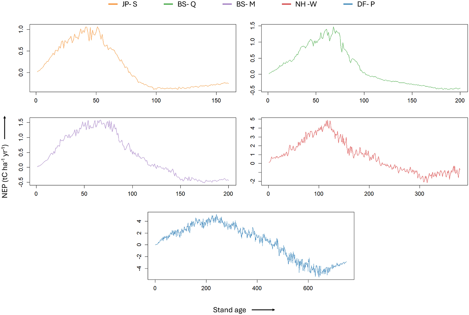
The NEP curves generated through Biome-BGCMuSo model simulations for each forest type, showing the dynamics of NEP over the lifespan of the forest. These curves demonstrate the NEP dynamics and align with Odum's theory: initial low NEP close to zero, a rise to a maximum during intermediate phase, and a decline to zero or negative in old-growth forests.
Figure 5

Best-fit polynomial curves for the simulated NEP data for the five sites, to outline the general trend curves. The curves are plotted against relative stand age for comparison. Shaded regions represent the uncertainty range around species-specific longevity estimates used to calculate relative stand age. Horizontal dashed lines near curve maxima indicate the range of relative stand ages corresponding to peak NEP, while dashed lines near NEP ≈ 0 denote the range of relative stand ages associated with the transition to near-neutral carbon balance.
The process-based modeling approach did not incorporate historical disturbances or initial carbon losses, which explains the absence of initial negative NEP in the simulations. This simplification was adopted due to the complexity of accurately modeling historical disturbances, especially for older sites where detailed disturbance data is often unavailable. As a result, while chronosequence data often exhibit negative NEP values during early post-disturbance stages, the model projections show low but positive NEP values in this period, likely leading to slight overestimation of NEP during early stand development. Our focus was on capturing long-term NEP dynamics across different forest types, particularly in mature and old-growth stages where the impact of initial disturbances on overall NEP trends is minimal. Despite this simplification, our model results align well with the chronosequence data, as demonstrated by the KS test results (Table 4).
Table 4
| Forest type | Comparison | D-statistic | P-value | RMSE | MAE |
|---|---|---|---|---|---|
| BS-M | EC vs. Modeled | 0.217 | 0.389 | 0.899 | 0.741 |
| BS-M | B vs. Modeled | 0.295 | 0.703 | 0.871 | 0.717 |
| BS-Q | EC vs. Modeled | 0.315 | 0.250 | 0.839 | 0.677 |
| JP-S | EC vs. Modeled | 0.342 | 0.063 | 0.645 | 0.535 |
| JP-S | B vs. Modeled | 0.481 | 0.390 | 0.682 | 0.568 |
| NH-W | EC vs. Modeled | 0.289 | 0.199 | 3.119 | 2.532 |
| DF-P | EC vs. Modeled | 0.162 | 0.340 | 4.300 | 3.486 |
Comparison of chronosequence data (B and EC methods) and modeled annual NEP from Biome-BGCMuSo using KS test, RMSE, and MAE metrics.
Modeled maximum NEP values at peak ages ranged from 1.05 to 5.09 tC ha−1 yr−1 across forest types. Figure 4 illustrates the modeled NEP curves for each forest type plotted against stand age. The simulation results also showed that forest ecosystems approached carbon neutrality (NEP≈0) between relative stand ages of approximately 0.46 and 0.86, with site-specific transitions occurring within the ranges shown in Table 3. Specifically, near-zero NEP conditions were observed between relative stand ages of 0.61–0.74 for BS-M, 0.57–0.69 for BS-Q, 0.71–0.86 for DF-P, 0.46–0.57 for JP-S, and 0.69–0.84 for NH-W. A modest increase or stabilization in NEP was observed during late-successional stages across all forest types, with varying magnitudes. This reflects a gradual decline in heterotrophic respiration as decomposition slows, soil organic matter becomes more recalcitrant, and microbial and nutrient cycling processes stabilize. The effect is most notably visible beyond 650 years in DF-P simulation, likely due to its extended longevity and larger soil carbon pools, which amplify the reduction in RH relative to other sites.
Figure 5 presents LOESS-smoothed NEP trajectories plotted against relative stand age, highlighting consistent NEP patterns across forest types and supporting Odum's conceptual model of ecosystem development. LOESS (Locally Estimated Scatterplot Smoothing) is a non-parametric method that fits local polynomial regressions across subsets of the data, making it well-suited for capturing general NEP trends without assuming a fixed global function. The inclusion of ±10% longevity variation bands accounts for uncertainty in species-specific lifespan estimates while preserving the broader trends in NEP dynamics across stand development stages.
To further validate NEP dynamics across biomes, we compared modeled outputs with EC flux tower data from southeastern U.S. forest sites (BL and ML). The modeled NEP curves for these sites aligned with the four hypothesized ecosystem development stages: (1) low NEP near zero in early development, (2) increasing NEP with intermediate stand age, (3) declining NEP in mature forests, and (4) fluctuating near-zero NEP during old growth (Figure 6).
Figure 6

The figure illustrates annual NEP curves for two sites, NEON Blandy Experimental Farm (BL) and NEON Mountain Lake Biological Station (ML), with different colored lines representing model output and black points for eddy covariance flux tower data. The top graph shows the ML site, while the bottom graph depicts the BL site. Inset 1:1 plots compare modeled and observed daily NEP values from eddy covariance (EC) data, demonstrating strong correlation between Biome-BGCMuSo model outputs and EC measurements. The daily and annual NEP EC data span 2017–2021 for the BL site and 2019–2021 for the ML site.
At the southeastern sites, model simulations indicated that peak NEP occurred at approximately 32 years of stand age for the BL site (representing upland hardwood forest) and 28 years for the ML site (representing bottomland hardwood forest), corresponding to relative stand age midpoints of 0.32 and 0.28, respectively, based on an estimated site and species-specific longevity of 100 years. Additionally, we included flux tower data from the southeastern US as referenced in (Metzger et al. 2019). For the BL site [NEON (National Ecological Observatory Network), 2023a], the net ecosystem exchange (NEE) values were recorded as follows: 2017: –232.66 gC m−2 yr−1, 2018: –346.74 gC m−2 yr−1, 2019: –269.00 gC m−2 yr−1, 2020: –500.02 gC m−2 yr−1, and 2021: –203.21 gC m−2 yr−1. For the ML site [NEON (National Ecological Observatory Network), 2023b], the NEE values were: 2019: –11.35 gC m−2 yr−1, 2020: –81.98 gC m−2 yr−1, and 2021: -68.43 gC m−2 yr−1. These NEE values represent the negative of the corresponding NEP values, providing a measure of the carbon flux at these sites.
The results from KS test, summarized in Table 4 indicate that for most sites, the null hypothesis that the Chronosequence data and Biome-BGCMuSo modeled NEP data come from the same continuous distribution cannot be rejected. This supports the model's reliability in predicting NEP trends across these forest types. However, for the Jack Pine site (JP-S EC vs. Modeled), the p-value was 0.0628, slightly above the typical significance threshold of 0.05. This suggests a marginal difference, likely due to the limited number of data points available for this site using the EC method, which includes only three data points. In contrast, the chronosequence data using B method for JP-S shows stronger agreement with a p-value of 0.3898. The limited data points for JP-S EC method highlight the importance of having comprehensive data for accurate validation of the model outputs. Overall, the KS test results support the robustness of the model in predicting NEP trends across different forest types.
To further evaluate model performance, we compared Root Mean Square Error (RMSE) and Mean Absolute Error (MAE) between modeled outputs and chronosequence observations. RMSE values for most sites ranged from 0.65 to 0.90 tC ha−1 yr−1, indicating good agreement in NEP magnitude, particularly for BS-M (0.87–0.90 tC ha−1 yr−1) and BS-Q (0.84 tC ha−1 yr−1). MAE values were consistently lower across all sites, ranging from 0.54 to 0.74 tC ha−1 yr−1, suggesting that average deviations between modeled and observed NEP remained moderate. In contrast, higher RMSE values were observed for NH-W (3.12 tC ha−1 yr−1) and DF-P (4.30 tC ha−1 yr−1), with correspondingly elevated MAE values of 2.53 and 3.49 tC ha−1 yr−1, respectively. The elevated errors for NH-W and DF-P partly reflect the temporal mismatch between observational years and simulated model years, as early stand development was simulated using recycled historical climate data due to the lack of site-specific records prior to 1980. This offset limits the ability to directly compare modeled and observed NEP on an annual basis. Additionally, old-growth systems inherently exhibit high year-to-year NEP variability due to heterogeneity in microclimate, and decomposition dynamics. Given these challenges, our validation emphasizes agreement in long-term age-related NEP trajectories, which the model captures robustly across forest types and disturbance histories. This is supported by the KS test, which evaluates the similarity in NEP distributions rather than year-to-year fluctuations, aligning with our objective of validating broader NEP trends across stand development. Thus, RMSE and MAE results should be interpreted as reflecting site-specific variability rather than systematic model bias, reinforcing the Biome-BGCMuSo model's overall robustness in simulating stand-scale NEP trajectories across contrasting forest types.
3.1 Sensitivity analysis
The sensitivity analysis demonstrated that atmospheric CO2 and nitrogen deposition have significant effects on NEP across all forest types. Comparing the core simulations (based on historical climate data) for chronosequence sites with both future climate data and static versus dynamic CO2 and nitrogen deposition scenarios (Figure 7), we observed key differences in NEP responses. The most notable difference was the magnitude of maximum NEP, which was substantially higher with dynamic CO2 and nitrogen deposition scenario compared to static and core simulations. In the core simulations, NEP trends follow a consistent pattern, where forests steadily sequester carbon, peaking at a specific range of relative stand ages across forest types. After this peak, NEP gradually declines to zero or transitions to a carbon source. However, the sensitivity analyses, which incorporate future climate projections, span only 150 years due to the limitations of available climate data and model projections. As a result, the NEP cycles in these analyses are incomplete, and the curves do not fully decline to zero by the end of the simulation period.
Figure 7

The NEP trends are shown across five different forest types: BS-M (Black Spruce - Manitoba), BS-Q (Black Spruce - Quebec), JP-S (Jack Pine - Saskatchewan), NH-W (Northern Hardwood - Wisconsin), and DF-P (Douglas Fir - Pacific Northwest). These trends are represented under three distinct scenarios. The first column illustrates core simulations conducted under historical climate conditions, where atmospheric CO2 is held constant at 290 ppm, along with a fixed nitrogen deposition rate (0.0005 kgN/m2/yr). The second column depicts simulations under future climate conditions while keeping CO2 and nitrogen deposition rates constant and same as the core simulations mentioned above. Finally, the third column shows simulations under future climate conditions with annually varying CO2 (310.65–538.35 ppm) and nitrogen deposition rates (0.00026–0.00096 kgN/m2/yr), based on published literature. Each scenario highlights the different responses of NEP to both static and dynamic atmospheric conditions.
The baseline simulations using historical climate data show smoother NEP trends, whereas future climate simulations exhibit greater variability, with sharp peaks and drops. These variations are plausible due to rapid changes in projected climate variables, such as more frequent extreme weather events. In simulations with annually varying CO2 and nitrogen deposition, NEP increases significantly, with peak levels occurring earlier than in static conditions, especially in younger stands. However, in most sites, the peak NEP is sustained for a longer period, indicating an extended phase of high productivity. This suggests that dynamic CO2 and nitrogen inputs not only accelerate carbon sequestration but also prolong the period of elevated productivity. Additionally, this scenario results in more pronounced NEP fluctuations.
Dynamic annually varying mortality rates have notable impact on NEP patterns. The sensitivity analysis, comparing constant mortality rates for each site with published standard dynamic mortality function (Merganičová and Merganič, 2014), reveals significant differences in NEP patterns. This comparison indicates that the dynamic mortality rates shift the timing and magnitude of NEP peaks, either delaying or advancing them relative to the constant mortality scenario. This finding supports the inclusion of dynamic mortality functions in our core simulations, as realistic mortality models are crucial for long term carbon dynamics projections.
Simulations with and without the spin-up phase revealed site-specific variability in NEP responses, with some sites exhibiting pronounced reductions in NEP while others showed only minor fluctuations. These results highlight the importance of including spin-up for stable and accurate NEP projections, particularly in long-term simulations. Compared to the sensitivity analyses of the spin-up phase, mortality rates, and atmospheric factors, EPC parameters had a smaller impact on model outcomes. Additional details on the sensitivity analyses of the spin-up phase and EPC parameters are provided in Supplementary Section 2. Among the EPC parameters, stomatal conductance exhibited the highest influence on NEP, causing a maximum change of 0.5 kgC m−2 yr−1 in the DF-P forest. In contrast, the sensitivity analysis comparing constant versus annually varying mortality rates showed a much larger effect on simulated NEP dynamics, resulting in a shift of 1.04 tC ha−1 yr−1 and moving the NEP peak from 35 to 56 years (1.63 to 0.59 tC ha−1 yr−1). This suggests that, although species-specific EPC parameters influence NEP and carbon dynamics, their effects are smaller compared to atmospheric concentration of CO2, nitrogen deposition and mortality rates.
4 Discussion
Our results provide quantitative, model based support for Odum's theory of ecosystem development and carbon dynamics in forest ecosystems. (Sprugel 1985) theorized that NEP is very small for old-growth forests, a pattern reflected in our model simulations and data synthesis. By incorporating species-specific longevity with a ±10% variability band, we found that NEP consistently peaked between relative stand ages of 0.24–0.39 across all forest types, with site-specific differences reflecting ecological and physiological traits. Jack Pine (JP-S), a fast-growing, short-lived species, peaked early (0.24–0.29) due to rapid canopy closure—consistent with post-fire chronosequence findings (Zha et al., 2009). In contrast, long-lived Douglas Fir (DF-P) peaked later (0.33–0.41), reflecting slower biomass accumulation and delayed canopy development (Law et al., 2003; Harmon et al., 2011). These trends align with known variation in stand density, carbon allocation, and mortality patterns (Fernández-Martínez et al., 2014; Coursolle et al., 2012). Even within same species, regional variation in climate and edaphic conditions shaped NEP trajectories, Black Spruce in Manitoba (BS-M), characterized by lower precipitation and more balanced soil texture (Harden et al., 2012), peaked earlier (0.29–0.35) than in Quebec (BS-Q, 0.31–0.38), where higher annual precipitation and finer-textured soils likely contributed to prolonged microbial activity and delayed NEP decline (Drobyshev et al., 2013). The gradual transition to near-zero NEP occurred between relative ages of 0.46–0.86, confirming that old-growth stages, across all forest types, tend toward carbon neutrality due to a balance between declining NPP and sustained or rising RH. These findings quantitatively support the theoretical model of ecosystem carbon flux and demonstrate that, despite species and site-level variations, forest types broadly follow a shared trajectory of net carbon uptake, peaking in mid-successional stages and stabilizing toward carbon neutrality in old growth. We acknowledge that the chronosequence sites in this study primarily represent boreal and temperate forests, including evergreen forest systems such as black spruce, jack pine, and Douglas-fir, with northern hardwoods as the only deciduous broadleaf-dominated chronosequence. To broaden biome representation, we incorporated model simulations and flux tower data from southeastern upland and bottomland hardwoods. The consistency in NEP-age trajectories across these deciduous systems supports the broader relevance of our findings. Still, expanding analyses to include diverse broadleaf forests from tropical, subtropical, and other underrepresented regions is necessary to strengthen broader ecological relevance.
The overall average NEP for old-growth ecosystems derived from chronosequence data was 0.13±0.29 tC ha−1 yr−1, which is significantly lower than the 2.4 tC ha−1 yr−1 reported by Luyssaert et al. (2008). This notable difference could be attributed to the following factors. First, our study utilized an average of five years of NEP data (ranging from 2 to 9 years), providing reliable estimation of NEP in old-growth forests, whereas Luyssaert et al. (2008) used shorter data periods, which likely contributed to their higher NEP estimates. For example, Luyssaert et al. (2008) reported one year NEP values > 1 tC ha−1 yr−1 for the northern hardwood and Douglas-fir sites, but our long-term data show both are carbon neutral. Second, our analysis incorporated data originating from forests affected by a single, stand-killing disturbance (e.g., harvest or wildfire), while the forests studied in Luyssaert et al. (2008) experienced two or more non-stand-killing disturbances and therefore were comprised of multi-age cohorts of the same or different tree species, potentially affecting their NEP estimates. Third, the definition of “old-growth” forests varies widely across ecosystems. While Luyssaert et al. (2008) used a uniform threshold of 200 years for defining old-growth, this approach overlooks the significant temporal variability in forest longevity and maturity. In contrast, our study accounts for species-specific longevity, providing a more nuanced and ecosystem-specific definition of old-growth.
Our sensitivity analysis provides important context for interpreting stand age–based NEP dynamics under changing environmental conditions. Simulations incorporating annually varying atmospheric CO2 and nitrogen deposition revealed earlier and more prolonged NEP peaks compared to static scenarios, suggesting that rising inputs can enhance mid-successional carbon uptake and extend productive phases. Dynamic mortality functions shifted both the timing and magnitude of NEP peaks, reinforcing the importance of realistic mortality modeling (Bugmann et al., 2019). Although ecophysiological parameters such as stomatal conductance had smaller effects, they still contributed to species-specific variation in NEP outcomes. Together, these results highlight the importance of integrating environmental sensitivity and model initialization when designing rotation ages or evaluating sequestration potential, particularly under future climate scenarios. They also underscore the value of scenario-based modeling for informing adaptive management and regionally tailored carbon strategies.
4.1 Implications for forest carbon management
Our findings have important implications for forest carbon management and climate change mitigation strategies. Contrary to some recent studies suggesting significant carbon sequestration in old-growth forests, our results indicate that these ecosystems tend toward carbon neutrality or weak net carbon sequestration as reflected in NEP, representing the balance between photosynthetic uptake and ecosystem respiration. This pattern primarily reflects living biomass and flux dynamics, while long-term soil carbon accumulation may follow different trajectories not captured by annual NEP. Nevertheless, the age-related decline in NEP is consistent with Odum's conceptual model and indicates a diminishing carbon sink strength after forest maturity. The strong relationship between stand age and NEP underscores the critical role of forest age structure in landscape-level carbon dynamics. This highlights the potential for strategic forest management to enhance carbon sequestration at regional scales. Notably, for some species, this peak NEP age aligns closely with typical rotation ages, while for others, there are significant variations. For northern hardwoods like sugar maple, with a lifespan of 300–400 years, peak NEP corresponds to ages of 98–119 years (0.32–0.39), broadly consistent with common even-aged management rotations of 80–120 years (Schuler, 1994; Wisconsin Department of Natural Resources, 2018). Similarly, black spruce, with a longevity of 250–300 years, exhibits peak NEP at 51–63 years, closely matching the typical rotation age of 60–90 years (Viereck and Johnston, 1990; Newton, 1998). Jack pine, with a lifespan of 150 years, reaches peak NEP at 32–39 years (0.24–0.29), slightly earlier than the standard 40–70 year rotations (Gadoth-Goodman and Rothstein, 2020; University of Minnesota Extension, 2018). In contrast, Douglas fir, with a longevity of 500–1,000 years, reaches peak NEP at 0.33–0.41 (198–246 years), far exceeding the typical harvest range of 40–120 years in the Pacific Northwest (Lowell et al., 2018). In Virginia's upland and bottomland hardwoods, species like red maple and black oak, with an approximate longevity of 100 years each, reach peak NEP at 28 and 32 years, earlier than the typical rotation ranges of 50–80 years (Rentch et al., 2009).
However, it is crucial to recognize that determining the ecological optimal age solely by peak NEP can be limiting. A more comprehensive approach is to examine the cumulative NEP curve and identify the point where its slope becomes minimal, indicating that sequestration rates (Annual change in rate of sequestration) have slowed, and the system is approaching a near-neutral carbon balance characteristic of old-growth stages. This approach accounts for initial carbon losses from respiration and highlights the age at which net carbon sequestration is optimized. By quantifying how carbon fluxes evolve with stand age, this study provides a practical foundation for aligning forest management with carbon objectives. Our results emphasize that forest age is not merely a structural attribute but a key driver of carbon dynamics, critical for optimizing sequestration outcomes. While our findings offer a scalable framework for carbon-focused management, further research is needed across forest types, regions, and climate scenarios to understand how NEP-age relationships vary with ecological conditions, management practices, and disturbance regimes. Furthermore, it is also important to recognize that this ecologically optimal age may differ significantly from economically optimal rotations. Economic models often prioritize maximizing timber yield or stocking, driven by assumptions about future market conditions, time preferences, and increasing disturbance risks in a changing climate. In particular, the inclusion of emissions fluxes from respiration at early ages is captured by ecosystem process modeling and flux tower sites but is typically not accounted for in economic modeling developed from forest inventories or field experiments.
The integrated modeling approach developed in this study offers valuable insights for forest management practices aimed at maximizing carbon sequestration while balancing other objectives such as forest preservation, soil health maintenance, and timber production. The low or negative NEP values observed in young stands underscore the importance of targeted site preparation and early stand management practices to limit emissions from respiration. Specifically, these practices include minimal soil disturbance techniques, such as avoiding mechanical tillage and retaining organic debris on the forest floor promotes organic matter retention, and reduces carbon losses during the early stand establishment phase (Mayer et al., 2020). Transitioning from clearcutting to more nature-friendly practices, such as shelterwood and selection systems, can help maintain NEP above zero by preserving forest structure and reducing soil disturbance (Puettmann et al., 2015; D'Amato et al., 2011). Additionally, selective harvesting methods that focus on removing individual trees or small groups help promote uneven-aged stand structures (D'Amato et al., 2011). This approach supports biodiversity and forest resilience by maintaining a variety of tree ages and species, which can enhance overall ecosystem stability and health (Merganič et al., 2020; Messier et al., 2019). These practices not only help reduce the duration and magnitude of the initial carbon source phase but also contribute to long-term forest health by stabilizing soil conditions and enhancing carbon sequestration (Peckham et al., 2012). The predictable pattern of NEP dynamics illustrates opportunities to combine process modeling with forest inventory assessments to support greenhouse gas (GHG) accounting for carbon offset projects (Hurteau et al., 2009).
It is important to note that this study does not undermine the ecological, cultural, and biodiversity value of old-growth forests. Rather, it contributes to our understanding of carbon dynamics in forest succession and provides insights for crucial decisions related to forest management, particularly on private lands and designated timberlands. In the United States, where forests offset approximately 12%–15% of annual greenhouse gas emissions (U.S. Environmental Protection Agency, 2022), improving the carbon sink capacity of managed forests could make a meaningful contribution to climate change mitigation efforts.
Our study provides valuable insights into temporal NEP dynamics, but it is important to acknowledge both the strengths and limitations of our modeling approach. The applied process-based model requires extensive site and species specific parameter inputs, which introduces challenges, particularly for historical periods with limited data availability. We addressed this by utilizing advanced geospatial data inputs and expert judgment to estimate initial conditions, which, while introducing some uncertainty, allowed us to create a comprehensive dataset to parameterize. We did not model disturbance legacies (e.g., initial C/N pools, soil water) and excluded early negative NEP to concentrate on influence of stand development, implying the early post-disturbance dynamics is underrepresented. Modeling approaches with site-specific initialization, as used in earlier intercomparison efforts (Hanson et al., 2004), could improve representation of early successional carbon dynamics in future work. For species-specific EPC parameters, especially for less-studied species, we employed a combination of literature values and calibration based on available flux tower data. Although this approach may not capture the full range of physiological responses across all sites and stand ages, it provided a robust foundation for our analysis. Because this analysis relies on a single process-based model structure, broader generality will benefit from evaluation across additional ecosystem models and mortality formulations, as emphasized in recent synthesis efforts (Fuller et al., 2025). A notable strength of this study lies in the long-term simulations conducted for species such as Douglas-fir (750 years) and northern hardwoods (350 years). To address the lack of continuous historical climate records over extended simulation periods, we employed a recycling strategy using 110–126 years of observed data to simulate early stand development. This approach captures general climate trends but reduces interannual variability, contributing to higher RMSE, MAE, and slope bias in 1:1 NEP validation plots at the BL and ML sites (Figure 6). However, these trade-offs are expected in long-term ecosystem modeling and do not affect our central objective of capturing broad-scale age-related NEP trajectories. The KS test results (Table 4) confirm that modeled NEP distributions align well with observed patterns, supporting the statistical robustness of long-term trends. Moreover, Biome-BGCMuSo's integration of microbial activity, decomposition, and nitrogen cycling provides critical process-level detail that enables ecologically realistic projections of carbon dynamics over decadal to centennial timescales, representing a significant advancement in modeling age-related trends in forest carbon balance.
A recently published synthesis paper provides an extensive evaluation of various ecological and economic models to assess their unique contributions to understanding forest carbon dynamics (Fuller et al., 2025). In addition, the outcomes of this research underscore the importance of accurately modeling ecosystem processes to predict responses to climate change and disturbances. Specifically, refining carbon sequestration estimates across stand ages and forest types, enhancing representations of old-growth carbon dynamics, and improving models to assess the effects of management practices on carbon sequestration across the lifespan of a stand (Zhao et al., 2022). By integrating these insights, stakeholders and policymakers can make more informed decisions about rotation ages, harvesting practices, and conservation strategies to optimize carbon sequestration at diverse spatial scales from stand level to landscape level. This integration would be particularly valuable for carbon offset projects and national greenhouse gas inventories, providing a more accurate assessment of forests' contributions to climate change mitigation efforts.
5 Conclusions
Our study provides quantitative support for long-standing ecological theories of forest development, finding consistent NEP trends and peaks across different North American Forest types. Our results are consistent with our ecological hypothesis that different forest types will experience peak NEP at similar relative stand ages. Our results, including sensitivity analysis of ecological factors on future NEP projections, offers new insights into optimal forest management for carbon sequestration (or other ecosystem services), including the potential temporal tradeoffs between managing forests for carbon at older relative stand ages, especially in disturbance-prone ecosystems.
Future research should focus on refining these findings across a broader range of forest types and climatic conditions, while focusing more on optimal management strategies (including rotations) under alternative future climate and nitrogen deposition scenarios consistent with different levels of socioeconomic development. Additionally, integrating these insights into improved landscape-scale forest management models will be crucial for applying this knowledge to climate change mitigation strategies at jurisdictional scales. By leveraging the natural carbon cycle of forests, informed by ecosystem process modeling, we can enhance their role in mitigating climate change while also meeting demand for forest products and other ecosystem services.
Statements
Data availability statement
The original contributions presented in the study are included in the article/Supplementary material, further inquiries can be directed to the corresponding author.
Author contributions
MG: Conceptualization, Data curation, Formal analysis, Investigation, Methodology, Visualization, Writing – original draft, Writing – review & editing. JB: Conceptualization, Funding acquisition, Investigation, Project administration, Resources, Supervision, Writing – original draft, Writing – review & editing. MA: Conceptualization, Investigation, Project administration, Resources, Supervision, Writing – original draft, Writing – review & editing. KM: Software, Supervision, Validation, Writing – original draft, Writing – review & editing.
Funding
The author(s) declared that financial support was received for this work and/or its publication. This research was funded by Jordan Family Graduate Fellowship for Natural Resource Innovation. KM was funded by the EU NextGenerationEU through the Recovery and Resilience Plan for Slovakia under the Project No. 09I03-03-V04-00130.
Acknowledgments
The authors are grateful for the early support and mentorship of Dr. Stith Tom Gower. Climate scenarios used were from the NEX-GDDP dataset, prepared by the Climate Analytics Group and NASA Ames Research Center using the NASA Earth Exchange, and distributed by the NASA Center for Climate Simulation (NCCS). Soil data for Canadian sites were derived from the Soil Landscapes of Canada (SLC) version 2.2, provided by the Centre for Land and Biological Resources Research, Research Branch, Agriculture and Agri-Food Canada, Ottawa, 1996. We acknowledge Agriculture and Agri-Food Canada's authorship of this dataset.
Conflict of interest
The author(s) declared that this work was conducted in the absence of any commercial or financial relationships that could be construed as a potential conflict of interest.
Generative AI statement
The author(s) declared that generative AI was not used in the creation of this manuscript.
Any alternative text (alt text) provided alongside figures in this article has been generated by Frontiers with the support of artificial intelligence and reasonable efforts have been made to ensure accuracy, including review by the authors wherever possible. If you identify any issues, please contact us.
Publisher’s note
All claims expressed in this article are solely those of the authors and do not necessarily represent those of their affiliated organizations, or those of the publisher, the editors and the reviewers. Any product that may be evaluated in this article, or claim that may be made by its manufacturer, is not guaranteed or endorsed by the publisher.
Supplementary material
The Supplementary Material for this article can be found online at: https://www.frontiersin.org/articles/10.3389/ffgc.2025.1702442/full#supplementary-material
References
1
Amiro B. D. Barr A. G. Barr J. G. Black T. A. Bracho R. Brown M. et al . (2010). Ecosystem carbon dioxide fluxes after disturbance in forests of North America. J. Geophys. Res. 115:1390. doi: 10.1029/2010JG001390
2
Batjes N. H. Calisto L. de Sousa L. M. (2024). Providing quality-assessed and standardised soil data to support global mapping and modelling (WoSIS snapshot 2023). Earth Syst. Sci. Data16, 4735–4765. doi: 10.5194/essd-16-4735-2024
3
Benish S. E. Bash J. O. Foley K. M. Appel K. W. Hogrefe C. Gilliam R. et al . (2022). Long-term regional trends of nitrogen and sulfur deposition in the United States from 2002 to 2017. Atmosphere. Chem. Phys. 22, 12749–12767. doi: 10.5194/acp-22-12749-2022
4
Besnard S. Carvalhais N. Arain M. A. Black A. de Bruin S. Buchmann N. et al . (2018). Quantifying the effect of forest age in annual net forest carbon balance. Environ. Res. Lett. 13:124018. doi: 10.1088/1748-9326/aaeaeb
5
Bond-Lamberty B. Wang C. Gower S. T. (2004). Contribution of root respiration to soil surface CO2 flux in a boreal black spruce chronosequence. Tree Physiol. 24, 1387–1395. doi: 10.1093/treephys/24.12.1387
6
Bugmann H. Seidl R. Hartig F. Bohn F. Brna J. Cailleret M. et al . (2019). Tree mortality submodels drive simulated long-term forest dynamics: assessing 15 models from the stand to global scale. Ecosphere10:e02616. doi: 10.1002/ecs2.2616
7
Burns R. M. Honkala B. (1990). Silvics of North America Vol. 1, Conifers and Vol. 2. Hardwoods, volume Agriculture handbook 654. Washington, DC: USDA Forest Service.
8
Canadell J. G. Raupach M. R. (2008). Managing forests for climate change mitigation. Science320, 1456–1457. doi: 10.1126/science.1155458
9
Carey E. V. Sala A. Keane R. Callaway R. M. (2001). Are old forests underestimated as global carbon sinks?Glob. Chang. Biol. 7, 339–344. doi: 10.1046/j.1365-2486.2001.00418.x
10
Centre for Land and Biological Resources Research (1996). Soil Landscapes of Canada, v.2.2. Technical Report, Research Branch, Agriculture and Agri-Food Canada, Ottawa.
11
Chang S. X. Shi Z. Thomas B. R. (2020). Soil respiration and net ecosystem productivity in a chronosequence of hybrid poplar plantations. Can. J. Soil Sci. 100, 488–502. doi: 10.1139/cjss-2020-0006
12
Chapin F. S. Woodwell G. M. Randerson J. T. Rastetter E. B. Lovett G. M. Baldocchi D. D. et al . (2006). Reconciling carbon-cycle concepts, terminology, and methods. Ecosystems9, 1041–1050. doi: 10.1007/s10021-005-0105-7
13
Cheng I. Zhang L. He Z. Cathcart H. Houle D. Cole A. et al . (2022). Long-term declines in atmospheric nitrogen and sulfur deposition reduce critical loads exceedances at multiple Canadian rural sites, 2000–2018. Atmosphere. Chem. Phys. 22, 14631–14656. doi: 10.5194/acp-22-14631-2022
14
Clark C. M. Phelan J. Ash J. Buckley J. Cajka J. Horn K. et al . (2023). Future climate change effects on US forest composition may offset benefits of reduced atmospheric deposition of N and S. Glob. Chang. Biol. 29, 4793–4810. doi: 10.1111/gcb.16817
15
Clarke L. Edmonds J. Jacoby H. Pitcher H. Reilly J. Richels R. (2007). Scenarios of Greenhouse Gas Emissions and Atmospheric Concentrations. Sub-Report 2.1a of Synthesis and Assessment Product 2.1, Department of Energy, Office of Biological &Environmental Research, Washington, DC.
16
Coursolle C. Margolis H. A. Giasson M. A. Bernier P. Y. Amiro B. D. Arain M. A. et al . (2012). Influence of stand age on the magnitude and seasonality of carbon fluxes in Canadian forests. Agric. Forest Meteorol. 165, 136–148. doi: 10.1016/j.agrformet.2012.06.011
17
D'Amato A. W. Bradford J. B. Fraver S. Palik B. J. (2011). Forest management for mitigation and adaptation: Insights from long-term silvicultural experiments. Forest Ecol. Manag. 262, 803–816. doi: 10.1016/j.foreco.2011.05.014
18
Desai A. R. Bolstad P. V. Cook B. D. Davis K. J. Carey E. V. (2005). Comparing net ecosystem exchange of carbon dioxide between an old-growth and mature forest in the upper Midwest, USA. Agric. Forest Meteorol. 128, 33–55. doi: 10.1016/j.agrformet.2004.09.005
19
Dobos R. R. Sinclair Jr H. R RobothamM. P. (2012). National commodity crop productivity index (NCCPI) user guide. Lincoln, Nebraska: User Guide, United States Department of Agriculture, Natural Resources Conservation Service.
20
Donner L. J. Wyman B. L. Hemler R. S. Horowitz L. W. Ming Y. Zhao M. et al . (2011). The dynamical core, physical parameterizations, and basic simulation characteristics of the atmospheric component AM3 of the GFDL global coupled model CM3. J. Clim. 24, 3484–3519. doi: 10.1175/2011JCLI3955.1
21
Drobyshev I. Gewehr S. Berninger F. Bergeron Y. (2013). Species specific growth responses of black spruce and trembling aspen may enhance resilience of boreal forest to climate change. J.Ecol. 101, 231–242. doi: 10.1111/1365-2745.12007
22
Dunn A. L. Barford C. C. Wofsy S. C. Goulden M. L. Daube B. C. (2007). A long-term record of carbon exchange in a boreal black spruce forest: Means, responses to interannual variability, and decadal trends. Glob. Chang. Biol. 13, 577–590. doi: 10.1111/j.1365-2486.2006.01221.x
23
Earth Resources Observation and Science (EROS) Center (2017). Shuttle Radar Topography Mission (SRTM) 1 Arc-Second Global. Reston, VA: U.S. Geological Survey. doi: 10.5066/F7PR7TFT
24
Environment and Climate Change Canada (2024). Historical Climate Data. Canadian Historical Daily Climate Data. Government of Canada. Available online at: https://climate.weather.gc.ca/ (Accessed September 30, 2024).
25
Fernández-Martínez M. Vicca S. Janssens I. A. Sardans J. Luyssaert S. Campioli M. et al . (2014). Nutrient availability as the key regulator of global forest carbon balance. Nat. Clim. Chang. 4, 471–476. doi: 10.1038/nclimate2177
26
Fuller M. R. Ganjam M. Baker J. S. Abt R. C. (2025). Advancing forest carbon projections requires improved convergence between ecological and economic models. Carbon Balance Manag. 20:2. doi: 10.1186/s13021-024-00290-0
27
Gadoth-Goodman D. Rothstein D. E. (2020). Alternative silvicultural approaches to managing jack pine plantations for endangered species habitat and forest products. Forest Sci. 66, 210–220. doi: 10.1093/forsci/fxz075
28
Goodbody T. R. H. Tompalski P. Coops N. C. White J. C. Wulder M. A. Sanelli M. (2020). Uncovering spatial and ecological variability in gap size frequency distributions in the Canadian boreal forest. Sci. Rep. 10, 1–12. doi: 10.1038/s41598-020-62878-z
29
Gough C. M. Vogel C. S. Schmid H. P. Curtis P. S. (2008). Controls on annual forest carbon storage: lessons from the past and predictions for the future. Bioscience58, 609–622. doi: 10.1641/B580708
30
Goulden M. L. Munger J. W. Fan S.-M. Daube B. C. Wofsy S. C. (1996). Measurements of carbon sequestration by long-term eddy covariance: methods and a critical evaluation of accuracy. Glob. Chang. Biol. 2, 169–182. doi: 10.1111/j.1365-2486.1996.tb00070.x
31
Gower S. T. McMurtrie R. E. Murty D. (1996). Aboveground net primary production decline with stand age: potential causes. Trends Ecol. Evol. 11, 378–382. doi: 10.1016/0169-5347(96)10042-2
32
Hanson P. J. Amthor J. S. Wullschleger S. D. Wilson K. B. Grant R. F. Hartley A. et al . (2004). Oak forest carbon and water simulations: model intercomparisons and evaluations against independent data. Ecol. Monogr. 74, 443–489. doi: 10.1890/03-4049
33
Harden J. W. Manies K. L. O'Donnell J. Johnson K. Frolking S. Fan Z. (2012). Spatiotemporal analysis of black spruce forest soils and implications for the fate of C. J. Geophys. Res. 117:1826. doi: 10.1029/2011JG001826
34
Harmon M. E. Bond-Lamberty B. Tang J. Vargas R. (2011). Heterotrophic respiration in disturbed forests: a review with examples from North America. J. Geophys. Res. 116:1495. doi: 10.1029/2010JG001495
35
Hartmann H. Trumbore S. (2016). Understanding the roles of nonstructural carbohydrates in forest trees-from what we can measure to what we want to know. New Phytol. 211, 386–403. doi: 10.1111/nph.13955
36
He L. Chen J. M. Pan Y. Birdsey R. Kattge J. (2012). Relationships between net primary productivity and forest stand age in U.S. forests. Global Biogeochem. Cycles26:3942. doi: 10.1029/2010GB003942
37
Hember R. (2018). “NACID - Nitrogen Deposition 1”, Mendeley Data, V1. doi: 10.17632/ktmg7xtt4j.1
38
Hidy D. Barcza Z. Haszpra L. Churkina G. Pintér K. Nagy Z. (2012). Development of the Biome-BGC model for simulation of managed herbaceous ecosystems. Ecol. Modell. 226, 99–119. doi: 10.1016/j.ecolmodel.2011.11.008
39
Hidy D. Barcza Z. Hollós R. Dobor L. Ács T. Zacháry D. et al . (2022). Soil-related developments of the Biome-BGCMuSo v6.2 terrestrial ecosystem model. Geosci. Model Dev. 15, 2157–2181. doi: 10.5194/gmd-15-2157-2022
40
Hidy D. Barcza Z. Marjanović H. Ostrogović Sever M. Z. Dobor L. Gelybó G. et al . (2016). Terrestrial ecosystem process model Biome-BGCMuSo v4.0: summary of improvements and new modeling possibilities. Geosci. Model Dev. 9, 4405–4437. doi: 10.5194/gmd-9-4405-2016
41
Hollós R. Kristóf E. Fodor N. Hidy D. Horváth F. Barcza Z. (2024). RBBGCMuso: an R Package to Support the Application of the Biome-BGCMuSo Biogeochemical Model. Available online at: https://github.com/hollorol/RBBGCMuso
42
Houtven G. V. Phelan J. Clark C. Sabo R. D. Buckley J. Thomas R. Q. et al . (2019). Nitrogen deposition and climate change effects on tree species composition and ecosystem services for a forest cohort. Ecol. Monogr. 89:e01345. doi: 10.1002/ecm.1345
43
Hurteau M. D. Hungate B. A. Koch G. W. (2009). Accounting for risk in valuing forest carbon offsets. Carbon Balance Manag. 4:1. doi: 10.1186/1750-0680-4-1
44
Janssens I. A. Dieleman W. Luyssaert S. Subke J.-A. Reichstein M. Ceulemans R. et al . (2010). Reduction of forest soil respiration in response to nitrogen deposition. Nat. Geosci. 3, 315–322. doi: 10.1038/ngeo844
45
Kira T. Shidei T. (1967). Primary production and turnover of organic matter in different forest ecosystems of the western pacific. Japanese J. Ecol. 17, 70–87.
46
Krishnan P. Black T. A. Jassal R. S. Chen B. Nesic Z. (2009). Interannual variability of the carbon balance of three different-aged Douglas-fir stands in the Pacific Northwest. J. Geophys. Res. 114:912. doi: 10.1029/2008JG000912
47
Lan X. Tans P. Thoning K. W. (2025). Trends in Globally-Averaged CO2Determined from NOAA Global Monitoring Laboratory Measurements. Version 2025-01. doi: 10.15138/9N0H-ZH07
48
Law B. E. Sun O. J. Campbell J. Van Tuyl S. Thornton P. E. (2003). Changes in carbon storage and fluxes in a chronosequence of ponderosa pine: changes in carbon storage. Glob. Chang. Biol. 9, 510–524. doi: 10.1046/j.1365-2486.2003.00624.x
49
Litvak M. Miller S. Wofsy S. C. Goulden M. (2003). Effect of stand age on whole ecosystem CO2 exchange in the Canadian boreal forest. J. Geophys. Res. 108:854. doi: 10.1029/2001JD000854
50
Lowell E. C. Turnblom E. C. Comnick J. M. Huang C. (2018). Effect of rotation age and thinning regime on visual and structural lumber grades of douglas-fir logs. Forests9:576. doi: 10.3390/f9090576
51
Luo H. Oechel W. C. Hastings S. J. Zulueta R. Qian Y. Kwon H. (2007). Mature semiarid chaparral ecosystems can be a significant sink for atmospheric carbon dioxide. Glob. Chang. Biol. 13, 386–396. doi: 10.1111/j.1365-2486.2006.01299.x
52
Luyssaert S. Schulze E. D. Börner A. Knohl A. Hessenmöller D. Law B. E. et al . (2008). Old-growth forests as global carbon sinks. Nature455, 213–215. doi: 10.1038/nature07276
53
Mayer M. Prescott C. E. Abaker W. E. Augusto L. Cécillon L. Ferreira G. W. et al . (2020). Tamm review: influence of forest management activities on soil organic carbon stocks: a knowledge synthesis. For. Ecol. Manage. 466:118127. doi: 10.1016/j.foreco.2020.118127
54
McKinney W. (2010). “Data structures for statistical computing in python,” in Python in Science Conference (Austin, Texas), 56–61. doi: 10.25080/Majora-92bf1922-00a
55
Menne M. J. Durre I. Korzeniewski B. McNeill S. Thomas K. Yin X. et al . (2012a). Global Historical Climatology Network - Daily (GHCN-Daily), Version 3. NOAA National Climatic Data Center. doi: 10.7289/V5D21VHZ
56
Menne M. J. Durre I. Vose R. S. Gleason B. E. Houston T. G. (2012b). An overview of the global historical climatology network-daily database. J. Atmosphere. Oceanic Technol. 29, 897–910. doi: 10.1175/JTECH-D-11-00103.1
57
Merganič J. Merganičová K. Výbošťok J. Valent P. Bahýľ J. Yousefpour R. (2020). Searching for pareto fronts for forest stand wind stability by incorporating timber and biodiversity values. Forests11:583. doi: 10.3390/f11050583
58
Merganicova K. (2004). Modelling forest dynamics in virgin and managed forest stands. Doctoral Thesis, BOKU - Universität für Bodenkultur Wien, Austria.
59
Merganičová K. Merganič J. (2014). The effect of dynamic mortality incorporated in biome-bgc on modelling the development of natural forests. J. Environ. Inf. 24, 24–31. doi: 10.3808/jei.201400273
60
Merganičová K. Merganič J. Dobor L. Hollós R. Barcza Z. Hidy D. et al . (2024). The biogeochemical model Biome-BGCMuSo v6.2 provides plausible and accurate simulations of the carbon cycle in central European beech forests. Geosci. Model Dev. 17, 7317–7346. doi: 10.5194/gmd-17-7317-2024
61
Merganičová K. Pietsch S. A. Hasenauer H. (2005). Testing mechanistic modeling to assess impacts of biomass removal. For. Ecol. Manage. 207, 37–57. doi: 10.1016/j.foreco.2004.10.017
62
Messier C. Bauhus J. Doyon F. Maure F. Sousa-Silva R. Nolet P. et al . (2019). The functional complex network approach to foster forest resilience to global changes. Forest Ecosyst. 6:21. doi: 10.1186/s40663-019-0166-2
63
Metzger S. Ayres E. Durden D. Florian C. Lee R. Lunch C. et al . (2019). From NEON field sites to data portal: a community resource for surface-atmosphere research comes online. Bull. Am. Meteorol. Soc. 100, 2305–2325. doi: 10.1175/BAMS-D-17-0307.1
64
National Atmospheric Deposition Program (2024). Total Deposition Maps README. Total Deposition Estimates Using the Measurement Model Fusion (TDep MMF version 2023.01) Approach with Modeled and Monitoring. Available online at: https://nadp.slh.wisc.edu/committees/tdep/ (Accessed April 17, 2024).
65
Nelson Institute Center for Climatic Research (2024). Wisconsin Historic Daily Climate data by Location. University of Wisconsin-Madison. Available online at: https://climatology.nelson.wisc.edu/wisconsin-historic-climate-data/daily-climate-data-by-location/ (Accessed December 20, 2024).
66
NEON (National Ecological Observatory Network) (2025). Vegetation Structure (DP1.10098.001), RELEASE-2025. Available online at: https://data.neonscience.org/data-products/DP1.10098.001/RELEASE-2025 (Accessed July 12, 2025).
67
NEON (National Ecological Observatory Network) (2023a). AmeriFlux FLUXNET-1F US-xBL NEON Blandy Experimental Farm (BLAN), Ver. 4-7, AmeriFlux AMP, (Dataset). doi: 10.17190/AMF/2229405
68
NEON (National Ecological Observatory Network) (2023b). AmeriFlux FLUXNET-1F US-xML NEON Mountain Lake Biological Station (MLBS), Ver. 4-7, AmeriFlux AMP, (Dataset). doi: 10.17190/AMF/1985447
69
Newton P. F. (1998). An integrated approach to deriving site-specific black spruce regeneration standards by management objective. For. Ecol. Manage. 102, 143–156. doi: 10.1016/S0378-1127(97)00153-9
70
Noguchi M. Hoshizaki K. Matsushita M. Sugiura D. Yagihashi T. Saitoh T. et al . (2022). Aboveground biomass increments over 26 years (1993–2019) in an old-growth cool-temperate forest in northern Japan. J. Plant Res. 135, 69–79. doi: 10.1007/s10265-021-01358-5
71
Noormets A. Chen J. Crow T. R. (2007). Age-dependent changes in ecosystem carbon fluxes in managed forests in Northern Wisconsin, USA. Ecosystems10, 187–203. doi: 10.1007/s10021-007-9018-y
72
Odum E. P. (1969). The strategy of ecosystem development. Science164, 262–270. doi: 10.1126/science.164.3877.262
73
Olea R. A. Pawlowsky-Glahn V. (2009). Kolmogorov-Smirnov test for spatially correlated data. Stochast. Environ. Res. Risk Assess. 23, 749–757. doi: 10.1007/s00477-008-0255-1
74
Ostrogović Sever M. Z. Barcza Z. Hidy D. Kern A. Dimoski D. Miko S. et al . (2021). Evaluation of the terrestrial ecosystem model biome-BGCMuSo for modelling soil organic carbon under different land uses. Land10:968. doi: 10.3390/land10090968
75
Ostrogović Sever M. Z. Paladinić E. Barcza Z. Hidy D. Kern A. Anić M. et al . (2017). Biogeochemical modelling vs. tree-ring measurements - comparison of growth dynamic estimates at two distinct oak forests in croatia. South-east Eur. Forest. 8, 71–84. doi: 10.15177/seefor.17-17
76
Peckham S. D. Gower S. T. Buongiorno J. (2012). Estimating the carbon budget and maximizing future carbon uptake for a temperate forest region in the U.S. Carbon Balance Manag. 7:6. doi: 10.1186/1750-0680-7-6
77
Peckham S. D. Gower S. T. Perry C. H. Wilson B. T. Stueve K. M. (2013). Modeling harvest and biomass removal effects on the forest carbon balance of the Midwest, USA. Environ. Sci. Policy25, 22–35. doi: 10.1016/j.envsci.2012.09.006
78
Peichl M. Brodeur J. J. Khomik M. Arain M. A. (2010). Biometric and eddy-covariance based estimates of carbon fluxes in an age-sequence of temperate pine forests. Agric. Forest Meteorol. 150, 952–965. doi: 10.1016/j.agrformet.2010.03.002
79
Peichl M. Martnez-Garca E. Fransson J. E. S. Wallerman J. Laudon H. Lundmark T. et al . (2023). Landscape variability of the carbon balance across managed boreal forests. Glob. Chang. Biol. 29, 1119–1132. doi: 10.1111/gcb.16534
80
Pietsch S. A. Hasenauer H. (2006). Evaluating the self-initialization procedure for large-scale ecosystem models. Glob. Chang. Biol. 12, 1658–1669. doi: 10.1111/j.1365-2486.2006.01211.x
81
Pregitzer K. S. Euskirchen E. S. (2004). Carbon cycling and storage in world forests: Biome patterns related to forest age. Glob. Chang. Biol. 10, 2052–2077. doi: 10.1111/j.1365-2486.2004.00866.x
82
Puettmann K. J. Wilson S. M. Baker S. C. Donoso P. J. Drössler L. Amente G. et al . (2015). Silvicultural alternatives to conventional even-aged forest management - what limits global adoption?Forest Ecosyst. 2:8. doi: 10.1186/s40663-015-0031-x
83
Rentch J. S. Miller G. W. Gottschalk K. W. (2009). Crown class dynamics of oaks, yellow-poplar, and red maple after commercial thinning in appalachian hardwoods: 20-year results. Northern J. Appl. Forest. 26, 156–163. doi: 10.1093/njaf/26.4.156
84
Running S. W. Hunt E. R. (1993). “Generalization of a forest ecosystem process model for other biomes, biome-bgc, and an application for global-scale models,” in Scaling Physiological Processes: Leaf to Globe, eds. J. R. Ehleringer, and C. B. Field (San Diego, CA: Academic Press), 141–158. doi: 10.1016/B978-0-12-233440-5.50014-2
85
Ryan M. G. (1991). Effects of climate change on plant respiration. Ecol. Applic. 1, 157–167. doi: 10.2307/1941808
86
Saiz G. Byrne K. A. Butterbach-Bahl K. Kiese R. Blujdea V. Farrell E. P. (2006). Stand age-related effects on soil respiration in a first rotation Sitka spruce chronosequence in central Ireland. Glob. Chang. Biol. 12, 1007–1020. doi: 10.1111/j.1365-2486.2006.01145.x
87
Schaaf C. Wang Z. (2021). MODIS/Terra+Aqua BRDF/Albedo Daily L3 Global - 500m V061. NASA EOSDIS Land Processes Distributed Active Archive Center (DAAC) data set, MCD43A3-061.
88
Schuler T. M. (1994). Survival, growth, and juvenile-mature correlations in a West Virginia sugar maple provenance test 25 years after establishment. Technical Report NE-RP-689, U.S. Department of Agriculture, Forest Service, North Central Research Station, St. Paul, MN. doi: 10.2737/NE-RP-689
89
Slonosky V. (2014). Historical climate observations in Canada: 18th and 19th century daily temperature from the St. Lawrence Valley, Quebec. Geosci. Data J. 1, 103–120. doi: 10.1002/gdj3.11
90
Smith S. J. Wigley T. (2006). Multi-gas forcing stabilization with minicam. Energy J. 27, 373–391. doi: 10.5547/ISSN0195-6574-EJ-VolSI2006-NoSI3-19
91
Soil Survey Staff (2024). Gridded Soil Survey Geographic (gSSURGO) Database for the Conterminous United States. United States Department of Agriculture, Natural Resources Conservation Service (202007 official release). Available online at: https://gdg.sc.egov.usda.gov/ (Accessed October 10, 2024).
92
Sprugel D. G. (1985). “Chapter 19 - natural disturbance and ecosystem energetics,” in The Ecology of Natural Disturbance and Patch Dynamics, eds. S. T. A. Pickett, and P. S. White (San Diego: Academic Press), 335–352. doi: 10.1016/B978-0-08-050495-7.50024-7
93
Streffing J. Sidorenko D. Semmler T. Zampieri L. Scholz P. Andrés-Martínez M. et al . (2022). AWI-CM3 coupled climate model: description and evaluation experiments for a prototype post-CMIP6 model. Geosci. Model Dev. 15, 6399–6427. doi: 10.5194/gmd-15-6399-2022
94
Tan Z.-H. Zhang Y.-P. Schaefer D. Yu G.-R. Liang N. Song Q.-H. (2011). An old-growth subtropical Asian evergreen forest as a large carbon sink. Atmos. Environ. 45, 1548–1554. doi: 10.1016/j.atmosenv.2010.12.041
95
Tang J. Bolstad P. V. Martin J. G. (2009). Soil carbon fluxes and stocks in a Great Lakes forest chronosequence. Glob. Chang. Biol. 15, 145–155. doi: 10.1111/j.1365-2486.2008.01741.x
96
Tang J. Luyssaert S. Richardson A. D. Kutsch W. Janssens I. A. (2014). Steeper declines in forest photosynthesis than respiration explain age-driven decreases in forest growth. Proc. Nat. Acad. Sci. 111, 8856–8860. doi: 10.1073/pnas.1320761111
97
Tedeschi V. Rey A. Manca G. Valentini R. Jarvis P. G. Borghetti M. (2006). Soil respiration in a Mediterranean oak forest at different developmental stages after coppicing. Glob. Chang. Biol. 12, 110–121. doi: 10.1111/j.1365-2486.2005.01081.x
98
The pandas development team (2020). Pandas-Dev/Pandas: Pandas. Zenodo. doi: 10.5281/zenodo.3509134
99
Thornton M. Shrestha R. Wei Y. Thornton P. Kao S.-C. (2022). DaymetDaymet: Daily Surface Weather Data on a 1-km Grid for North America. Version 4 R1.
100
Thornton P. E. Running S. W. (1999). An improved algorithm for estimating incident daily solar radiation from measurements of temperature, humidity, and precipitation. Agric. Forest Meteorol. 93, 211–228. doi: 10.1016/S0168-1923(98)00126-9
101
Thrasher B. Maurer E. P. McKellar C. Duffy P. B. (2012). Technical Note: Bias correcting climate model simulated daily temperature extremes with quantile mapping. Hydrol. Earth Syst. Sci. 16, 3309–3314. doi: 10.5194/hess-16-3309-2012
102
U.S. Environmental Protection Agency (2022). EPA (2022) Inventory of U.S. Greenhouse Gas Emissions and Sinks: 1990-2020. Technical Report EPA 430-R-22-003. Washington, DC: U.S. Environmental Protection Agency. Available online at: https://www.epa.gov/ghgemissions/inventory-us-greenhouse-gas-emissions-and-sinks
103
University of Minnesota Extension (2018). Managing Jack Pine Forests. Available online at: https://extension.umn.edu/managing-woodlands/managing-jack-pine-forests (Accessed April 2, 2025).
104
Viereck L. A. Johnston W. F. (1990). “Picea mariana (Mill.) B. S. P. Black Spruce,” in Silvics of North America: Volume 1. Conifers, eds. R. M. Burns, and B. H. Honkala (Washington, DC: United States Department of Agriculture, Forest Service), 227–237.
105
Wharton S. Falk M. Bible K. Schroeder M. Paw U K. (2012). Old-growth CO2 flux measurements reveal high sensitivity to climate anomalies across seasonal, annual and decadal time scales. Agric. Forest Meteorol. 161, 1–14. doi: 10.1016/j.agrformet.2012.03.007
106
White M. A. Thornton P. E. Running S. W. Nemani R. R. (2000). Parameterization and sensitivity analysis of the BIOME-BGC terrestrial ecosystem model: net primary production controls. Earth Inter. 4, 1–85. doi: 10.1175/1087-3562(2000)004<0003:PASAOT>2.0.CO;2
107
Wilkins K. Clark C. Aherne J. (2022). Ecological thresholds under atmospheric nitrogen deposition for 1200 herbaceous species and 24 communities across the US. Glob. Chang. Biol. 28:2381. doi: 10.1111/gcb.16076
108
Wisconsin Department of Natural Resources (2018). Wisconsin Silviculture Guide. Technical Report FR-805–40, Wisconsin Department of Natural Resources, Madison, WI.
109
Wise M. Calvin K. Thomson A. Clarke L. Bond-Lamberty B. Sands R. et al . (2009). Implications of limiting CO2 concentrations for land use and energy. Science324, 1183–1186. doi: 10.1126/science.1168475
110
Zha T. Barr A. G. Black T. A. McCAUGHEY J. H. Bhatti J. Hawthorne I. et al . (2009). Carbon sequestration in boreal jack pine stands following harvesting. Glob. Chang. Biol. 15, 1475–1487. doi: 10.1111/j.1365-2486.2008.01817.x
111
Zhao J. Lange H. Meissner H. (2022). Estimating carbon sink strength of Norway spruce forests using machine learning. Forests13:1721. doi: 10.3390/f13101721
112
Zhou L. Dai L. Wang S. Huang X. Wang X. Qi L. et al . (2011). Changes in carbon density for three old-growth forests on Changbai Mountain, Northeast China: 1981–2010. Ann. For. Sci. 68, 953–958. doi: 10.1007/s13595-011-0101-3
Summary
Keywords
biogeochemical cycle modeling, climate change impacts, ecosystem modeling, forest carbon dynamics, net ecosystem productivity (NEP), soil respiration, stand age development
Citation
Ganjam M, Baker JS, Aguilos M and Merganičová K (2026) Maximizing net ecosystem productivity: integrating chronosequence analysis and ecosystem modeling across contrasting biomes in North America. Front. For. Glob. Change 8:1702442. doi: 10.3389/ffgc.2025.1702442
Received
16 September 2025
Revised
19 December 2025
Accepted
30 December 2025
Published
27 January 2026
Volume
8 - 2025
Edited by
Chenxi Li, Xi'an University of Architecture and Technology, China
Reviewed by
Xiaojie Gao, Harvard University, United States
Yueh-hsin Lo, National Dong Hwa University, Taiwan
Updates
Copyright
© 2026 Ganjam, Baker, Aguilos and Merganičová.
This is an open-access article distributed under the terms of the Creative Commons Attribution License (CC BY). The use, distribution or reproduction in other forums is permitted, provided the original author(s) and the copyright owner(s) are credited and that the original publication in this journal is cited, in accordance with accepted academic practice. No use, distribution or reproduction is permitted which does not comply with these terms.
*Correspondence: Manaswini Ganjam, mganjam@ncsu.edu
† Present address: Manaswini Ganjam, Centre for Tree Ring Science, University of Missouri, Columbia, MO, United States
Disclaimer
All claims expressed in this article are solely those of the authors and do not necessarily represent those of their affiliated organizations, or those of the publisher, the editors and the reviewers. Any product that may be evaluated in this article or claim that may be made by its manufacturer is not guaranteed or endorsed by the publisher.