Representing unsegmented vessels using available vascular data for bioheat transfer simulation

Introduction: A primary challenge with voxel domains generated from imaging data is associated with voxel resolution. Due to the dimensional scale of blood vessels, not all vessels are captured in a given voxel resolution, leading to discontinuous blood vessels in the segmentation. Pre-capillary vessels like arterioles, which provide the highest resistance to blood flow, are often modeled with tissue as a porous domain due to resolution limitations. This results in a loss of information that could have been modeled if these vessels were segmented and modeled distinctly from the capillary bed.

Methods: This paper focuses on developing mathematical equations to calculate the flow resistance of unsegmented vasculature with reference to flow resistance of available segmented vascular data. A 3D vascular domain of 32 terminal vessels and five generations of bifurcation is simulated. Each generation is successively removed and substituted with the new flow resistance equations to analyze the error in heat transfer due to a lack of segmentation data.

Results: The effect of using mathematical equations of flow resistance on bioheat transfer is analyzed. Two methods are proposed and demonstrated to show considerable error reduction in bioheat transfer.

Discussion: Very high image resolution, which could allow modeling of pre-capillary vessels, increases the computational cost of the entire simulation domain. Instead, a mathematical representation of the pressure drop induced in these unsegmented blood vessels is used. The proposed methods show potential in reducing the error resulting from the lack of segmentation data, improving the accuracy of bioheat transfer simulations.

Introduction

Technological advancements enable visualization and modeling of the vasculature (Ivilinov Todorov et al., 2020; Silvestri et al., 2021), providing highly detailed blood vessel domains. When coupled with accurate biophysics simulations (Amare et al., 2022; Blowers et al., 2018), such realistic models can be used to illustrate, understand, and predict biological responses to different environmental conditions. Such tools can predict patient response to medical treatment, changes in blood flow distribution due to burns or clots (Ng and Chua, 2002a; Ng and Chua, 2002b; Cookson et al., 2012), drug distribution, and damage to healthy tissue during hyperthermia treatments (Bellizzi et al., 2020; Silva et al., 2020).

However, a very high resolution data maybe required depending on the scale of domain size. The resolution of the voxel domain limits the visualization of blood vessels that can be modeled. Although capillary beds can be modeled using the porous media assumption in tissue (Amare et al., 2022; Hodneland et al., 2019), pre-capillary vessels that impact heat transfer (Weinbaum and Jiji, 1985; Lemons et al., 1987; Jiji et al., 1984) also play a crucial role in vasomotion. The arterioles, which can vary flow resistance, are present in pre-capillary vessels that often get overlooked in bioheat transfer. For an accurate and thorough simulation of biophysics, the ability to simulate the effects of arterioles is important; thus, modeling the pre-capillary network is crucial.

In a voxel domain generated from imaging data, a blood vessel ends where the resolution of the voxel can no longer identify it. One option to simulate the pre-capillary vessels from this point would be the mathematical modeling of blood vessels or an algorithm to simulate vascularization. Vascularization and angiogenesis are highly complex phenomena that include chemical, physical, and biological processes (Tran et al., 2022; Stefanini et al., 2012; Corada et al., 2014; Chappell et al., 2019; Tang et al., 2014). Vascular Endothelial Growth Factor (VEGF) signaling released by the tissue cells directs the tip cell to guide vascularization. Various biocomputational models have been developed to simulate this process (Takigawa-imamura et al., 2022; Kim et al., 2012; Heck et al., 2015; Zhang et al., 2022). However, computational models developed from a biological perspective (Zhang et al., 2022) are different from models developed from an engineering perspective. One of the primary approaches engineers use to model blood vessel growth is modeling blood vessels as fractals (Merks and Glazier, 2006; Tong and Fan, 2001; Murray, 2003a; Murray, 2003b; Lorthois and Cassot, 2010; Niemeyer et al., 1984) like the Diffusion Aggregation Method proposed by Fleury (Vincent and Schwartz, 1999; Vincent and Schwartz, 2000; Witten and Sander, 1981).

Another engineering method used to simulate vascularization is called Constrained Constructive Optimization (CCO) (Schreiner, 1993; Schreiner et al., 1995; Schreiner et al., 2006; Cury et al., 2021). In CCO, the main assumption is that blood flow is equally distributed in the specific organ domain. Based on this assumption, the supply blood flow rate in the organ is equally distributed in a given number of terminals. The blood flow rate passing through a single terminal vessel and the pressure drop between the supply node and the terminal of vasculature are provided as constraints. A random point is selected within the domain and a new branch is grown towards the point. The radius of the new branch is calculated such that the total volume of the vasculature is minimized. The CCO method has undergone various modifications such as parallelizing the growth of blood vessels (Talou et al., 2021; Cury et al., 2021; Shen et al., 2021) to increase computational efficiency. An example of the application of the CCO model is found in Correa-Alfonso’s work of vascularization on mesh liver model (Correa-Alfonso et al., 2022). The minimum diameter of a blood vessel in this liver model is 100 μm. The blood vessels in this model are shunted, i.e., arteries are directly connected with veins. The shunt between arteries and veins at 100 μm cannot model the time blood spends in the capillary bed. Blood flow is the slowest in the capillary bed and is expected to have a higher energy absorption rate due to the time spent there. The challenge with using the CCO method with a voxel phantom is associated with voxel resolution. For example, in the mesh liver model, to model the blood vessels of diameter 500 μm, a voxel resolution of less than 100 μm is required. When a cuboidal voxel of size 100 μm is used to voxelize the mesh, the liver model has a total of $1.36\times 10^7$ voxels; and about 70% of hepatic arteries are lost in the voxelization of the liver mesh as they have a diameter of less than 500 μm.

Modeling every blood vessel to the capillary bed is not a feasible solution. Thus, a new method is required to model the flow resistance and heat transfer of blood vessels that exist between the capillary bed and the segmented blood vessels. In previous work (Amare et al., 2022; Hodneland et al., 2019) a multiscale, mixed-dimensional simulation framework was developed for simulating multiphysics, known as the VoM-PhyS framework. This framework uses a pressure drop parameter (Hodneland et al., 2016; Hodneland et al., 2019) to simulate the resistance of the “virtual” blood vessels that are not segmented. However, no in-vivo or empirical data are available to determine the pressure drop parameter. In previous work (Amare et al., 2023) a 2D domain was studied and the major findings were: (1) The flow resistance of unsegmented vessels can be recovered using the pressure drop parameter in the VoM-PhyS framework; (2) A constrained range was observed within which the correct pressure drop parameter value exists for a given simulation domain; and (3) The error in flow and pressure maps due to lack of segmented vessels can be reduced with the use of correct pressure drop parameter. This paper focuses on expanding on these findings for a 3D domain with the following aims: (1) Provide equations to calculate the correct pressure drop parameter for any available vascular domain; (2) Study the effect of unsegmented vessels on bioheat transfer in the VoM-PhyS framework; and (3) Provide rectification methods to reduce the temperature error.

This study aims to address three key challenges in bioheat transfer modeling: (1) Develop mathematical equations to calculate the pressure drop parameter for unsegmented vasculature using only net flow rate and flow resistance of segmented vessels. (2) Quantify the effect of unsegmented vessels on bioheat transfer simulations. (3) Propose and evaluate methods to reduce temperature errors in bioheat simulations with limited vascular data. The novelty of this work lies in: (a) The development of a mathematical framework to represent unsegmented vessels, bridging the gap between high-resolution vascular modeling and practical imaging limitations. (b) Demonstration of the impact of unsegmented vessels on bioheat transfer simulations, highlighting that correcting flow resistance alone is insufficient for accurate heat transfer modeling. (c) Proposal of two methods to reduce temperature errors: implementing an effective thermal conductivity approach and assuming equal spatial distribution from terminal vessels.

Methods

For this research, the VoM-PhyS framework was used to simulate blood flow coupled with heat transfer. The pressure drop parameter, $\gamma$, is an important parameter in the VoM-PhyS framework that permits modeling the unsegmented pre-capillary vessels. The ratio of blood viscosity $(\mu )$ and pressure drop parameter $(\gamma )$ is an empirical representation of flow resistance offered by unsegmented blood vessels. A detailed description of this parameter can be found in (Hodneland et al., 2019; Amare et al., 2022). The goal of this work is to provide mathematical equations to calculate $\gamma$. To derive the equations for $\gamma$, a blood vessel domain generated using the CCO algorithm with the assumption of equal flow distribution in the domain was used. This domain is shown in Figure 1. In the VoM-PhyS framework, the porous tissue domain is modeled as two-compartments, arterial and venous, and coupled using the perfusion parameter, $\alpha$. The arterial pressure drop parameter, ${\gamma }_a$, controls the flow resistance of unsegmented blood vessels between arterial terminal nodes 3 and arterial compartment pressure nodes. Similarly, the venous pressure drop parameter, ${\gamma }_v$, controls the flow resistance between venous compartment pressure nodes and venous terminal pressure nodes 4.

Figure 1

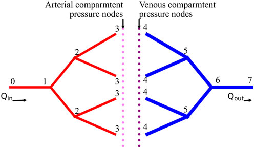
Figure 1. Example domain illustration.

Step 1: mass conservation and total flow

The blood flow rate flowing in the volume is ${\mathcal{Q}}_{in}$ from the arterial side, and the blood flow rate leaving the domain is ${\mathcal{Q}}_{\mathit{out}}$, respectively. Since mass is conserved, ${\mathcal{Q}}_{in}$ is equal to ${\mathcal{Q}}_{\mathit{out}}$ as shown in Equation 1. In Figure 1, the arteries (red) and veins (blue) are considered to be the segmented vasculature for which the length and diameter can be calculated from imaging data.

$\mathcal{Q}={\mathcal{Q}}_{in}={\mathcal{Q}}_{\mathit{out}}(1)$

The blood entering the tissue domain is considered to be uniformly distributed (Schreiner, 1993; Schreiner et al., 1995; Xing et al., 2022; Correa-Alfonso et al., 2022). Thus, the flow rates leaving the arterial terminal nodes $3$ are considered to be equal. With the equal distribution assumption, the blood flow rates in the terminal vessels are calculated using Equation 2, where $n$ represents the number of bifurcation generations. In the illustrated example, $n$ is equal to 2.

${\mathcal{Q}}_{\mathit{term}}=\frac{\mathcal{Q}}{2^n}(2)$

Step 2: define equivalent resistances and pressure drops

Using the dimensions of the vasculature, the equivalent flow resistance offered by each arterial and venous vascular tree can be calculated using parallel and series resistance methods. The equivalent resistance of arterial and venous trees are represented as ${\mathcal{R}}_A$ and ${\mathcal{R}}_V$, respectively, and shown in Figure 2. Figure 2 represents the simplification of the domain from Figure 1 by calculating equivalent flow resistances of segmented arteries and veins.

Figure 2

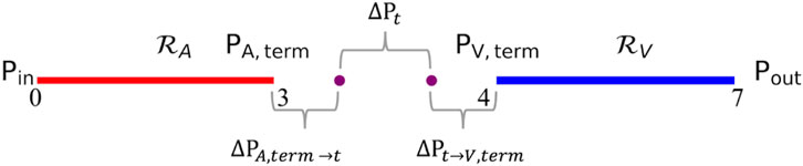
Figure 2. Simplified domain.

Using the simplified blood vessel model, the blood flow equations in the arterial and venous trees can be written as Equation 3 and Equation 4, respectively. $P_{A,term}$ represents the pressure at node 3 where the segmented arteries end, and $P_{V,term}$ represents the pressure at node 4 where the segmented veins end.

$P_{A,term}=P_{in}-\mathcal{Q}{\mathcal{R}}_A(3)$

$P_{V,term}=P_{\mathit{out}}+\mathcal{Q}{\mathcal{R}}_V(4)$

The total pressure drop between terminal arteries and terminal veins represents the pressure drop across unsegmented vasculature. This pressure drop can be calculated using Equation 5, where $\mathrm{\Delta }{P}_{A,term\to t}$ and $\mathrm{\Delta }{P}_{t\to V,term}$ represent the pressure drop between the terminal artery and arterial compartment and venous compartment and terminal vein, respectively. $\mathrm{\Delta }{P}_t$ represents the pressure drop across arterial and venous compartments within the tissue and is calculated using the perfusion coefficient, $\alpha$, and total volume, $V$, of the tissue domain as shown in Equation 6.

$P_{A,term}-P_{V,term}=\mathrm{\Delta }{P}_{\mathit{term}}=\mathrm{\Delta }{P}_{A,term\to t}+\mathrm{\Delta }{P}_t+\mathrm{\Delta }{P}_{t\to V,term}(5)$

$\mathrm{\Delta }{P}_t=\frac{\mathcal{Q}}{\alpha V}(6)$

Step 3: correlation between resistances and pressure drop

A correlation between the flow resistance of arterial and venous trees and the pressure drop between terminal vessels and tissue is proposed in Equation 7. The correlation states that the ratio of pressure drop between unsegmented arteries to capillary bed and unsegmented veins to capillary bed is equal to the ratio of overall flow resistance offered by segmented arteries and veins. The constand $\psi$ is used for derivation only and it represents the ratio of effective arterial resistance to effective venous resistance.

$\frac{\mathrm{\Delta }{P}_{A,term\to t}}{\mathrm{\Delta }{P}_{t\to V,term}}=\left[\frac{{\mathcal{R}}_A}{{\mathcal{R}}_V}\right]=\psi (7)$

$\mathrm{\Delta }{P}_{A,term\to t}=\psi \mathrm{\Delta }{P}_{t\to V,term}(8)$

Using Equation 8 and substituting in Equation 5, equations for $\mathrm{\Delta }{P}_{A,term\to t}$ and $\mathrm{\Delta }{P}_{t\to V,term}$ are derived, shown in Equation 9 and Equation 10, respectively.

$\mathrm{\Delta }{P}_{A,term\to t}=\frac{\psi \left(\mathrm{\Delta }{P}_{\mathit{term}}-\mathrm{\Delta }{P}_t\right)}{\left(\psi +1\right)}(9)$

$\mathrm{\Delta }{P}_{t\to V,term}=\frac{\left(\mathrm{\Delta }{P}_{\mathit{term}}-\mathrm{\Delta }{P}_t\right)}{\left(\psi +1\right)}(10)$

Step 4: solve for pressure drop parameters

The resistance equation for flow in virtual vessels can be written as Equations 11, 12 where the resistance offered by virtual arterial and venous networks is represented using blood viscosity $\mu$ and pressure drop parameter ${\gamma }_{\beta }$.

$\mathrm{\Delta }{P}_{A,term\to t}={\mathcal{Q}}_{A,term}\frac{\mu }{{\gamma }_a}(11)$

$\mathrm{\Delta }{P}_{t\to V,term}={\mathcal{Q}}_{V,term}\frac{\mu }{{\gamma }_v}(12)$

Using Equations 9–12, the equations to determine pressure drop parameter for the arterial and venous tree is derived as shown in Equation 13 and Equation 14, respectively.

${\gamma }_a=\frac{\mu \mathcal{Q}}{2^n}\frac{\left(\frac{{\mathcal{R}}_A}{{\mathcal{R}}_V}+1\right)}{\frac{{\mathcal{R}}_A}{{\mathcal{R}}_V}\left[\mathrm{\Delta }P-\mathcal{Q}\left[{\mathcal{R}}_A+{\mathcal{R}}_V+{\left(\alpha V\right)}^{-1}\right]\right]}(13)$

${\gamma }_v=\frac{\mu \mathcal{Q}}{2^n}\frac{\left(\frac{{\mathcal{R}}_A}{{\mathcal{R}}_V}+1\right)}{\left[\mathrm{\Delta }P-\mathcal{Q}\left[{\mathcal{R}}_A+{\mathcal{R}}_V+{\left(\alpha V\right)}^{-1}\right]\right]}(14)$

Equation 13 and Equation 14 are the final forms of equations to calculate the pressure drop parameter for arterial and venous trees. It can be seen from these equations that the pressure drop parameters can be calculated using total blood flow rate in the simulation domain, pressure drop across the simulation domain, and the equivalent resistance of arterial and venous trees calculated from the segmented vasculature. The demonstration of how to use the pressure drop equations for a given biological domain is shown in Figure 3.

Figure 3

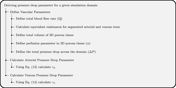
Figure 3. Flowchart illustrating the steps for using pressure drop parameter equations.

3D domain

To verify the applicability of the Equation 13 and Equation 14 on a 3D domain, a test domain shown in Figure 4 was generated using Rhinoceros (McNeel et al., 2010). The domain has 32 terminals for arterial and venous trees and the cuboidal tissue size encasing the vasculature was $20$ $\mathrm{c}\mathrm{m}$ × $20$ $\mathrm{c}\mathrm{m}$ × $20$ $\mathrm{c}\mathrm{m}$. The voxel dimensions are $2.5$ $\mathrm{m}\mathrm{m}$ × $2.5$ $\mathrm{m}\mathrm{m}$ × $2.5$ $\mathrm{m}\mathrm{m}$. The 32 terminal domain was considered as a reference solution (most segmented data available) for comparison and will be referred to as Case 1. Similar to previous work (Amare et al., 2023) on a 2D domain, the number of terminals was reduced gradually to create different simulation domains representing lack of segmented data as shown in Figure 4. The resultant domains are termed Case 2, Case 3, Case 4, and Case 5 for 16, 8, 4, and 2 terminals, respectively (Figure 4). The dimensions of the arterial and venous trees were considered same for this simulation for simplicity and are given in Table 1.

Figure 4

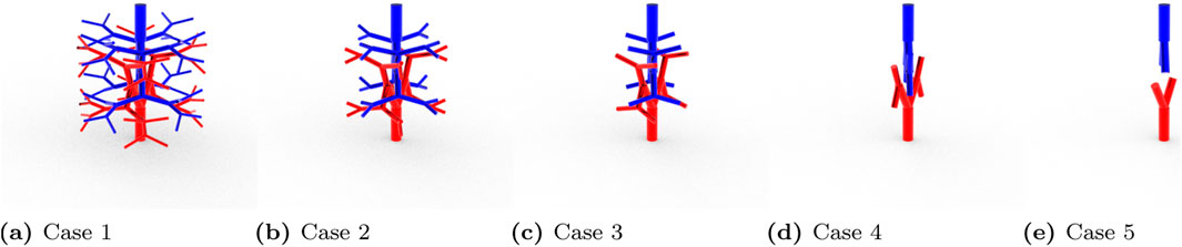
Figure 4. 3D simulation domain cases. (A) Case 1, (B) Case 2, (C) Case 3, (D) Case 4, (E) Case 5.

Table 1

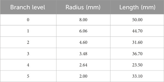
Table 1. Dimensions of vasculature in 3D Domain.

Since this was a 3D modeled domain, a reference volumetric blood flow rate had to be determined. The VoM-PhyS framework (Amare et al., 2022; Hodneland et al., 2019) was used with the flow parameters given in Table 2 to calculate the overall volumetric blood flow rate in Case 1. The pressure drop parameter for this simulation was considered as $1$ ${\mathrm{m}}^3$. This ensured that only the flow resistance of segmented vessels in Case 1 determine the overall blood flow rate.

Table 2

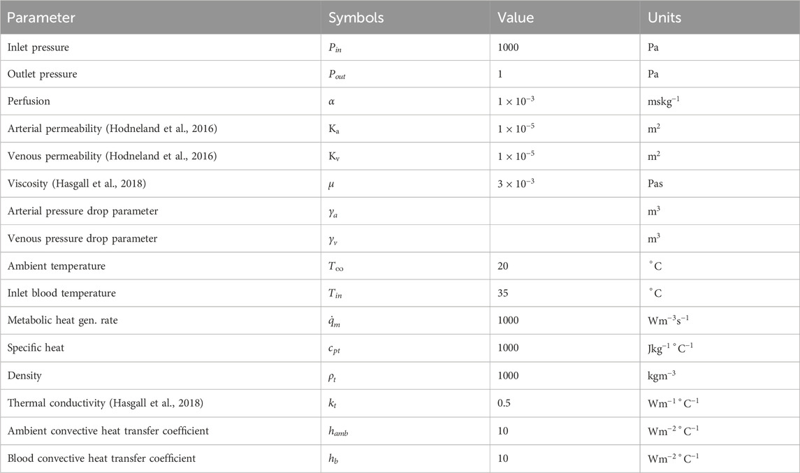
Table 2. Parameters used for 3D blood flow and heat transfer simulation.

The parameters used in this 3D blood flow and heat transfer simulation model are based on established physiological values and commonly accepted approximations in biomedical engineering. The blood viscosity $(\mu )$ and thermal conductivity $(k_t)$ are consistent with values reported in the IT’IS database for biological tissues (Hasgall et al., 2018). The arterial and venous permeability values ($K_a$, $K_v$) are supported by previous computational models of tissue perfusion (Amare et al., 2022; Hodneland et al., 2016; Hodneland et al., 2019). The perfusion rate $(\alpha )$ falls within the typical range for various tissue types (Jeong et al., 2023). The specific heat $(c_{pt})$ and density $({\rho }_t)$ of the tissue are approximated to those of water, a common practice in biological heat transfer models (Duck, 2013). The ambient temperature $(T_{\infty })$ represents a standard room temperature, while the inlet blood temperature $(T_{in})$ is slightly below core body temperature, accounting for cooler peripheral blood. The metabolic heat generation rate is within the range observed in various tissues, albeit on the higher end (Wahyudi et al., 2022). The convective heat transfer coefficients for ambient and blood ($h_{\mathit{amb}}$, $h_b$) are typical values used in biological heat transfer simulations. While the inlet and outlet pressures are lower than physiological arterial pressures, they are representative for the specific modeling conditions and simulate a pressure drop of arround $1000$ $\mathrm{P}\mathrm{a}$ (Timothy, 2016; Li et al., 2012).

Using Equations 13, 14, the pressure drop parameters for all five cases were calculated. The blood flow was simulated with the respective pressure drop parameters and the pressure maps were compared with the reference Case 1.

Pressure drop parameter equations

The pressure drop parameters calculated using Equation 13 and Equation 14 for the 3D reference domain (Figure 4) are shown in Table 3. Nt represents the number of vascular terminals for respective cases. To understand the importance of pressure drop parameter and its effect on pressure solution, Figure 5 is shown. Here the percentage error in pressure at arterial nodes $6$, $5$, and $4$ of Case 2 is plotted for $\pm$1%, $\pm$2%, and $\pm$5% change in ${\gamma }_a$. Nodes 5 represent the last segemnted node in Case 2, Nodes 4 represent the nodes connected to Nodes 5, and Nodes 3 represent the pressure nodes connected to Nodes 4. There are many biological factors like non-newtonian behavior of blood and vasomotion which are not considered in Equations 13, 14. Thus, these equations can only provide an accurate flow resistance behavior of unsegmented vessels. A 0.6% change in pressure for 5% in pressudre drop parameter can be seen from Figure 5. This shows that an accurate pressure drop parameter will be sufficient for preliminary analysis and simulation of blood flow.

Table 3

Table 3. Pressure drop parameters calculated using Equation 13 and Equation 14 for 3D domain.

Figure 5

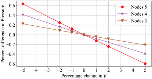
Figure 5. Effect of pressure drop parameter on simulation result in Case 2 compared with Case 1.

The flow equations were solved using the pressure drop parameters of respective cases and pramaters shown in Table 2. The resultant pressure values are given in Tables 4–6, for the arterial tree, venous tree, and tissue compartments, respectively. In Table 6, the average, maximum, and minimum pressures in the arterial and venous compartment of all the cases is shown. A contour map for pressure error between Cases 2 to 5 and Case 1, is shown in Figure 6, at z = 80 the location of z in the domain shown in Figure 7. The pressure difference between Case 5 and Case 1 at each tissue voxel is within $\pm$$0.75$ $\mathrm{P}\mathrm{a}$. Case 5 represents the worst case possible with the least segmented vasculature available.

Table 4

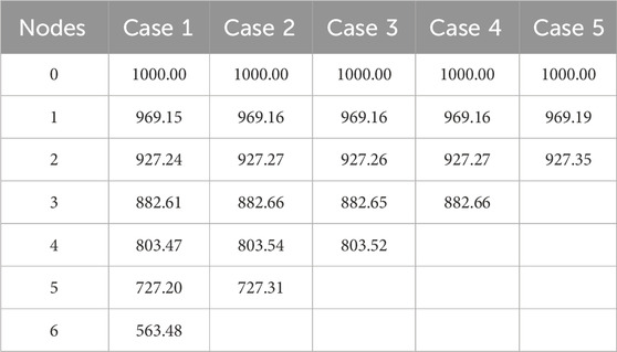
Table 4. Pressure ($\mathrm{P}\mathrm{a}$) in arterial tree.

Table 5

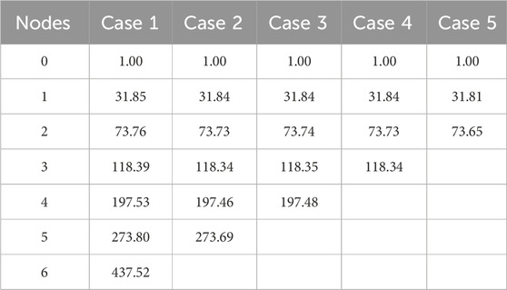
Table 5. Pressure ($\mathrm{P}\mathrm{a}$) in venous tree.

Table 6

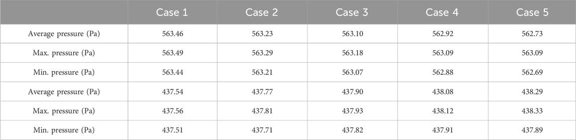
Table 6. Pressure ($\mathrm{P}\mathrm{a}$) in tissue compartments.

Figure 6

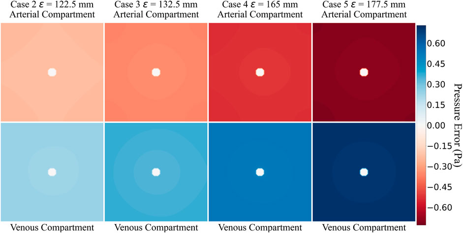
Figure 6. Pressure error analysis.

Figure 7

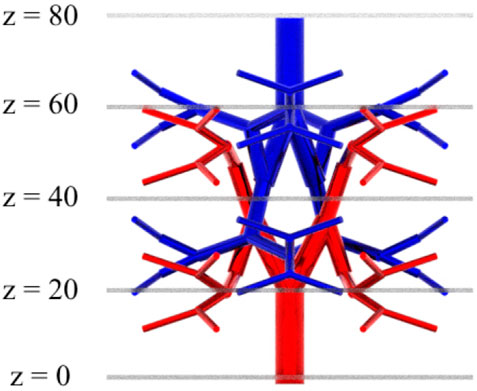
Figure 7. Location of z.

Bioheat transfer

To analyse the effect of lack of segmentation data on bioheat transfer, Case 1 temperature profile was considered as reference solution, and all other Cases were compared to it. The temperature errors of Case 2, Case 3, Case 4, and Case 5 at z = $80$ are shown in Figure 8. The location of z = 80 was selected as it had the maximum temperature error in the entire domain. The dimensionless temperature error was calculated using Equation 15. $T_{\mathit{amb}}$ represents the ambient temperature used for simulation, $T_{in}$ represents the inlet blood temperature, $T_{\mathit{ref,i}}$ represents the temperature of ith voxel in Case 1, and $T_{c,i}$ represents the temperature of ith voxel in Case c where c $\in (\mathrm{2,3,4,5})$.

${\theta }_i=\frac{T_{c,i}-T_{\mathit{ref,i}}}{T_{in}-T_{\mathit{amb}}}(15)$

Figure 8

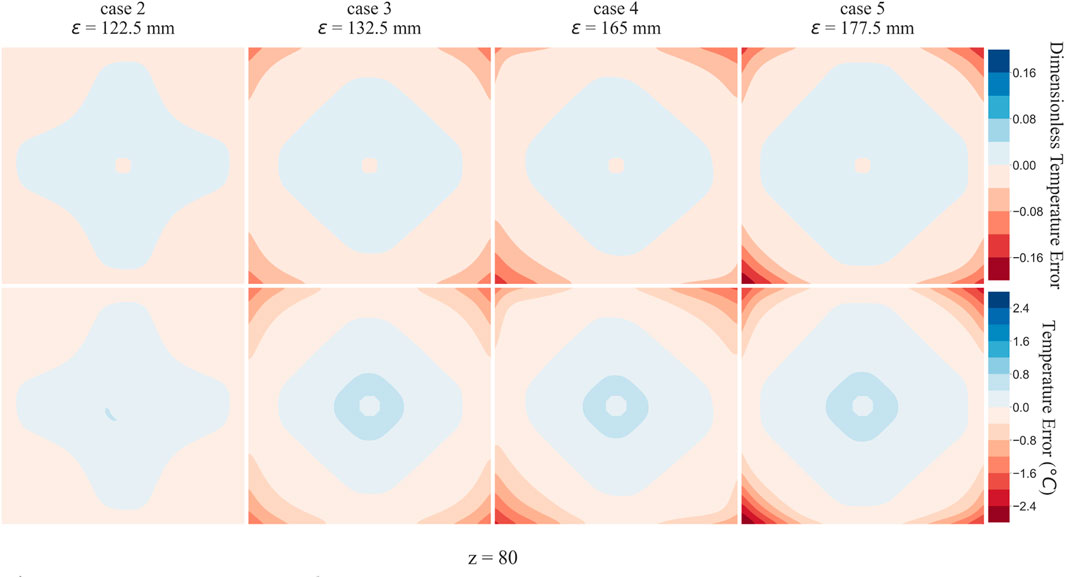
Figure 8. Temperature error analysis.

Discussion

Tables 4, 5 show that with the use of the correct value for the pressure drop parameter, the flow resistance of the unsegmented vessels can be simulated and the pressure drop in the vascular tree can be accurately determined. For Case 5, which represents the worst-case scenario with only two terminal arteries and veins, the pressure contours in the arterial and venous compartments of tissue show a maximum pressure error of $\pm 0.72$ $\mathrm{P}\mathrm{a}$. The corresponding error is less than 0.5% when compared to the arterial and venous compartment pressure values in reference Case 1.

The greatest flow resistance for a blood is at arterioles. These pre-capillary arterioles are not always captured in the segmented data. Any change in the flow resistance of these pre-capillaries would result in changes in total flow rate and pressure drop. In the example under consideration, since the pressure drop across the domain is given as boundary condition, the pressure drop parameter affects the total blood flow rate, as shown in the previous work (Amare et al., 2023). The pressure drop parameter thus controls an important aspect in the VoM-PhyS framework. A small change in pressure drop parameter changes the pressure drop across the vascular tree. A local vasomotion can be simulated by varying the pressure drop parameter of respective vessel terminal.

The pressure difference between Case 5 and Case 1 at each tissue voxel is within $\pm$$0.75$ $\mathrm{p}\mathrm{a}\mathrm{s}\mathrm{c}\mathrm{a}\mathrm{l}$ and negligible, the temperature difference between these two cases is within $\pm$2.5°C as shown in Figure 8. This temperature difference is substantial and cannot be ignored. Thus, correcting flow resistance alone does not guarantee reduction in bioheat simulation error. Blood vessels are considered to affect heat transfer via countercurrent flow (Weinbaum et al., 1984). When vessels are unsegmented, their effect on surrounding tissue cannot be simulated. To minimize this temperature error, two methods were considered: effective thermal conductivity and larger Sphere of Influence (SoI) radius (Amare et al., 2022; Amare et al., 2023).

Effective thermal conductivity

Between two tissue voxels, heat transfer takes place via advection and conduction. As the blood flows from one porous tissue voxel to another, it carries the heat with it resulting in advection. As the pressure map was consistent with maximum error within $\pm 0.75$ $\mathrm{P}\mathrm{a}$, there was negligible change in the flow rate among tissue voxels. However, as fewer blood vessels are segmented, they are modeled as part of tissue porosity. The porous tissue voxels now consist of larger blood vessel than the reference domain (Case 1). Though there was no change in heat transfer due to advection, thermal conduction among tissue voxels can change due to larger unsegmented vessels. In literature (Chen and Holmes, 1980; Keller and Seiler, 1971; Weinbaum et al., 1984; Weinbaum and Jiji, 1985; Roetzel and Xuan, 1997; Nakayama and Kuwahara, 2008), effective thermal conductivity is used to consider the effect of unsegmented blood vessels and counter-current heat exchange. The same concept of effective thermal conductivity was used to compensate for the effect of cross-flow heat exchange between unsegmented blood vessels. The thermal conductivity of the tissue voxels was varied between $0.5{\mathrm{W}\mathrm{m}}^{-1}{}^{◦}◦\mathrm{C}^{-1}$ to $2.0{\mathrm{W}\mathrm{m}}^{-1}{}^{◦}◦\mathrm{C}^{-1}$. The resultant temperature errors between Case 5 and Case 1 for different values of tissue thermal conductivity are shown in Table 7 with the temperature contours plots at z = 80 shown in Figure 9. From Figure 9 and Table 7 it can be seen that as the tissue thermal conductivity increases, the temperature error begins to reduce till it reaches a threshold value, beyond which the temperature error seems to increase.

Table 7

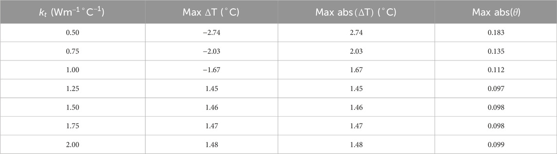
Table 7. Effect of tissue thermal conductivity on temperature error.

Figure 9

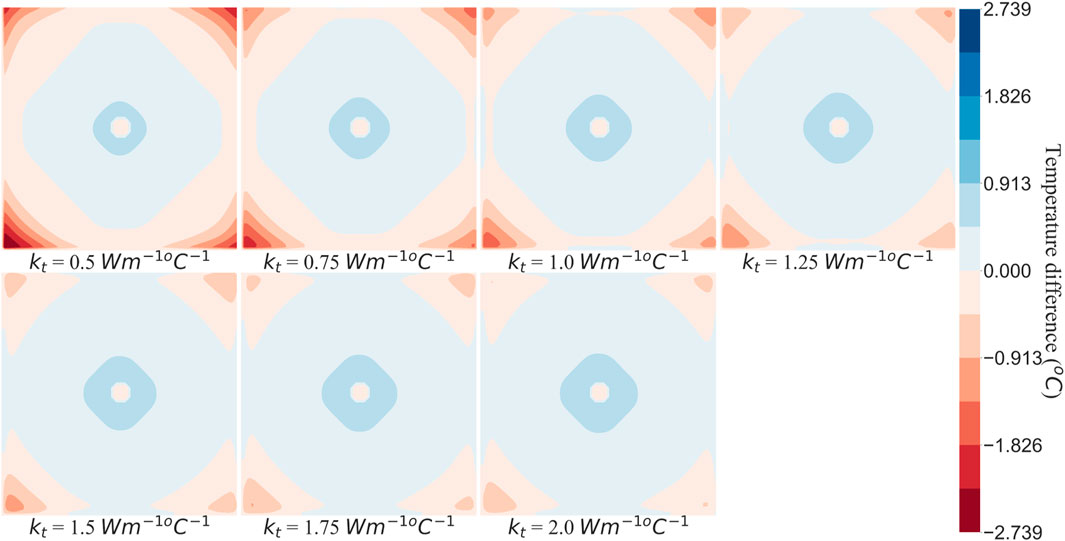
Figure 9. Effect of thermal conductivity at z = 80 for $ϵ=$ $177.5$ $\mathrm{m}\mathrm{m}$

Larger SoI

Sphere of Influence (SoI) is a parameter introduced in previous work (Hodneland et al., 2016; Hodneland et al., 2019) and is critical in the VoM-PhyS framework (Amare et al., 2022) for coupling 1D flow with 3D flow. The SoI is a volume of sphere with origin center at a terminal vessel. The tissue voxels that fall within a given SoI are considered to exchange blood with the respective terminal vessel. The radius, $ϵ$, of the SoI is an empirical quantity. The effect of $ϵ$ on blood flow and pressure drop was studied (Amare et al., 2023) and $ϵ$ did not demonstrate any effect on pressure drop. However, $ϵ$ has been shown to affect thermal maps in tissue (Amare et al., 2022). Thus, different values of $ϵ$ were studied to understand its effect on reduction of temperature error due to unsegmented vessels. The temperature error values for different $ϵ$ and different values of tissue thermal conductivity, $k_t$, are given in Tables 8, 9. The temperature difference contours at z = 80 for Case 5 with $k_t$ as $0.5$ $\mathrm{W}{\mathrm{m}}^{-1}{◦\mathrm{C}}^{-1}$ is shown for different values of $ϵ$. From Table 8 and Figure 10, it can be seen that as the $ϵ$ increases, the temperature error begins to decrease and reaches a threshold value beyond which there is no change in the temperature error. This behavior is different than the effect of $k_t$, where beyond the threshold, the temperature error begins to increase again.

Table 8

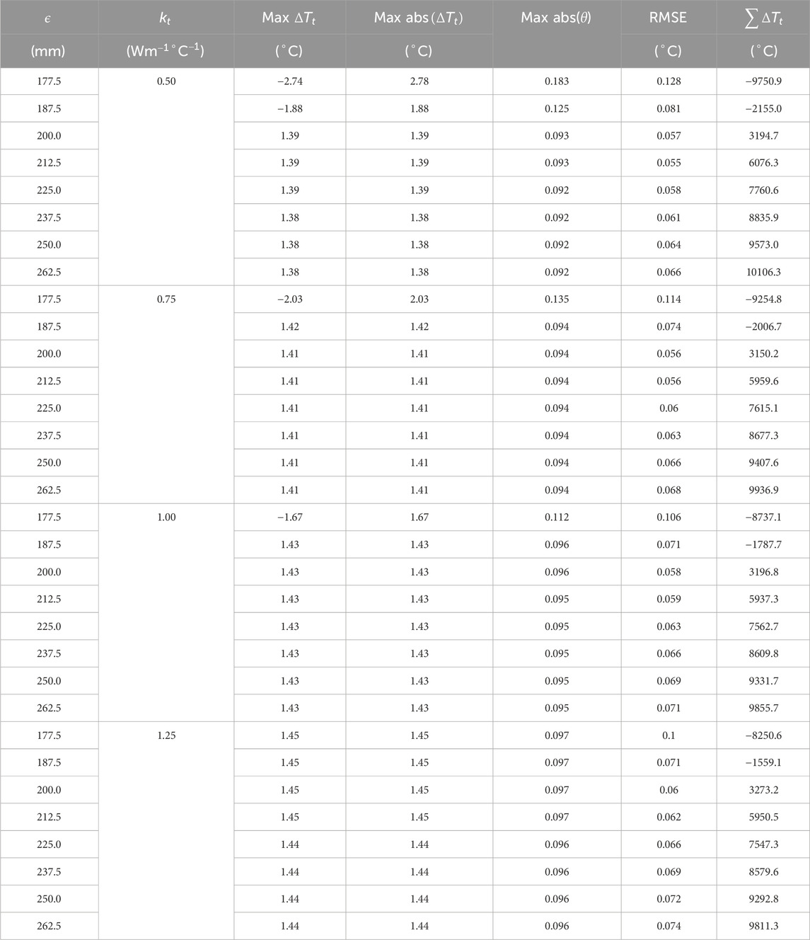
Table 8. Effect of larger SoI and tissue thermal conductivity on temperature error.

Table 9

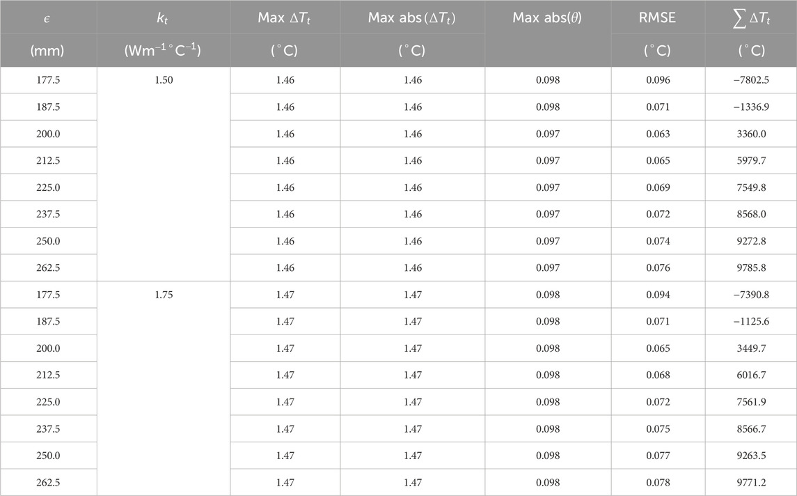
Table 9. Effect of larger SoI and tissue thermal conductivity on temperature error.

Figure 10

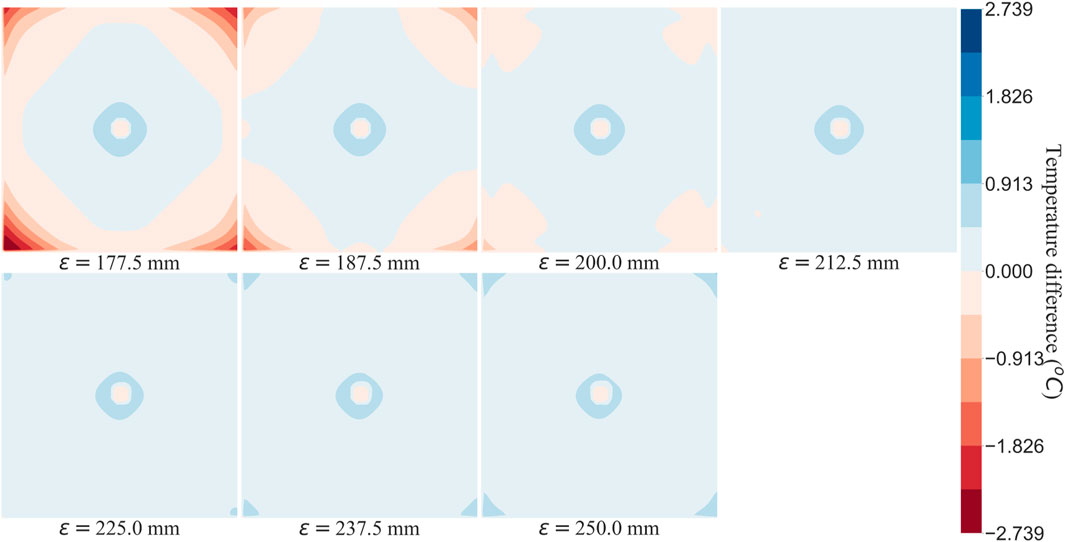
Figure 10. Effect of larger SoI at z = 80 for $k_t=$ $0.5{\mathrm{W}\mathrm{m}}^{-1}{}^{◦}\mathrm{C}^{-1}$

To understand the effect of these two methods on temperature error reduction, root mean square error (RMSE) and the sum of temperature error (STE) in the entire domain were calculated. The values of RMSE and STE are shown in Tables 8, 9, and a graphical plot of RMSE and $\sum \mathrm{\Delta }{T}_t$ for the different values of $k_t$ and $ϵ$ is shown in Figures 11, 12, respectively. In Figure 11, it can be seen that as $k_t$ increases, the RMSE decreases for $ϵ$ to a threshold value. Beyond the threshold, the RMSE increases with an increase in $k_t$. Using polynomial regression, six polynomial functions of the fourth order were fitted for RMSE for each value of $k_t$, respectively. Similarly, six polynomial functions of fourth order were fitted for STE for each value of $k_t$. Using the RMSE function, the threshold where minimum RMSE occurs was calculated, along with the corresponding STE. These values are given in Table 10. It is noteworthy that the STE is positive for all $k_t$ at the threshold $ϵ$ of minimum RMSE. This denotes that the VoM-PhyS framework would result in higher temperatures than the reference for a less segmented vascular domain. Similarly, the $ϵ$ where STE equals zero was calculated along with the corresponding RMSE. These values are given in Table 11. The values of $ϵ$ where STE is zero are not the same where minimum RMSE occurs, as can be seen. A further detailed statistical analysis of these values could lead to greater insight into the performance of the proposed energy error reduction methods. A further analysis is needed to determine what parameters affect the value of $ϵ$ for any given vascular data. Another noteworthy observation is that the minimum temperature for larger SoI is for $k_t=$ $0.5$ $\mathrm{W}{\mathrm{m}}^{-1}{◦\mathrm{C}}^{-1}$, and this error increases for the same SoI when tissue thermal conductivity is varied. A SoI larger than the minimum required for 100% coverage ensures the tissue domain lies closer to the source than the periphery of the SoI. This provides more blood flow to the entire tissue domain than the simulation case when SoI is restricted to minimum $ϵ$ for 100% coverage. As the SoI is increased, it is expected to achieve equal distribution in the entire tissue domain, and is expected when the SoI is considerably larger than the domain dimensions. This behavior ensures that we reach a plateau beyond which the temperature error cannot be decreased even if the SoI is increased.

Figure 11

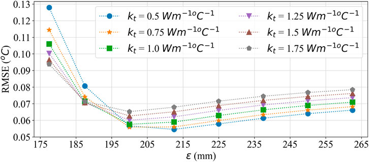
Figure 11. RMSE plot for comparing the effect of effective thermal conductivity and larger SoI on temperature error.

Figure 12

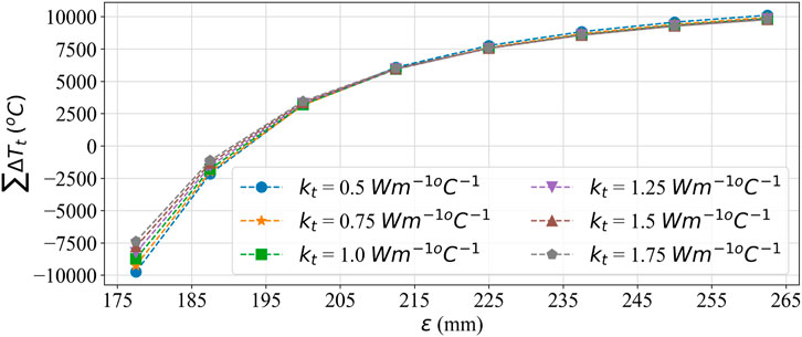
Figure 12. Summation error plot for comparing the effect of effective thermal conductivity and larger SoI on temperature error.

Table 10

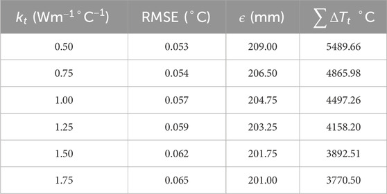
Table 10. Threshold value of $ϵ$ and the corresponding summation of temperature error for Case 5.

Table 11

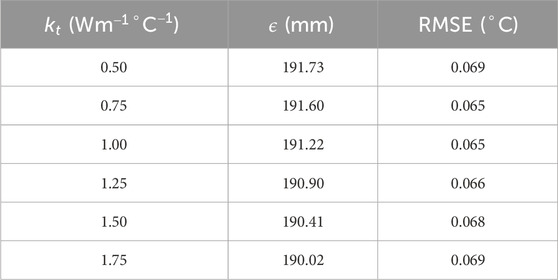
Table 11. Value of $ϵ$ where summation of temperature error in Case 5 equals to zero and the resultant RMSE.

The use of the equations to calculate correct pressure drop parameter for a given vasculature opens avenues for furthering this research field. Availability of segmentable vascular model remains a challenge, but the use of the pressure drop parameter equation provides a novel way to overcome this challenge and obtain a detailed accurate blood flow simulation. This study clearly shows the effect of unsegmented vasculature is dominant on heat transfer simulation. Further research is required to better understand methods to quantify this error and be able to provide rectification methods from available data. Similar to the equations proposed in this paper for calculating pressure drop parameter, if equations to rectify the temperature error could be derived, that would provide a major revolution in the field. Such equations could help simulate large scale domains which otherwise could not be easily modeled due to their computational memory requirement.

These findings also highlight that correcting flow resistance alone is insufficient for accurate heat transfer modeling. This insight is critical for researchers developing bioheat transfer models, as it underscores the need for additional considerations beyond flow resistance.

One of the major limitation of this work is tied to the SoI. The SoI is an empirical value and no data is available to determine its accuracy. The SoI radius is expected to vary based on the biological domain under consideration, tissue properties, vasomotion, and various other biological features. A detail study is required to better understand this parameter.

To derive the equations of pressure drop parameter, a simulation domain where segmented vasculature could be gradually removed was required. Obtaining such a simulation domain from medical imaging data still remains a challenge as discussed in the Introduction. The resolution of image required to get the desired segmentable vasculature is very high, increasing the computational overhead for simulation. The pressure drop parameter itself is the solution to model flow resistance of unsegmented blood vessels and hence an artificial 3D domain with blood vessels was developed for derivation of mathematical equations. Future work will include demonstrating the use of these equations on biological organs obtained from medical imaging scans.

While our proposed methods significantly improve bioheat transfer simulations with limited vascular data, several limitations should be noted. The pressure drop parameter equations assume steady-state flow and do not account for pulsatile effects or non-Newtonian blood behavior. The effectiveness of the error reduction methods may vary depending on the specific organ or tissue being modeled. Additionally, validation against in vivo measurements remains challenging due to the complexity of obtaining high-resolution temperature data in living tissues.

The broader implications of this work extend to various fields. In medical applications, more accurate bioheat transfer models could improve the planning and execution of thermal therapies, such as hyperthermia treatments for cancer. Our current research focuses on this and will be published in future work. In physiological research, these methods could enhance our understanding of thermoregulation in different organs. For computational biology, our approach offers a pathway to simulate large-scale domains that were previously computationally prohibitive, potentially enabling more comprehensive whole-organ or even full-body simulations.

These findings provide novel equations to calculate the pressure drop parameter $(\gamma )$ for unsegmented vasculature using only the net flow rate and flow resistance of segmented vessels. This advancement allows for accurate pressure mapping in simulations with limited vascular network data, addressing a significant challenge in the field. The study provides a detailed analysis of how the lack of segmented vascular data affects temperature profiles in bioheat transfer simulations and proposes two approaches to mitigate these errors: implementing an effective thermal conductivity approach and assuming equal spatial distribution from terminal vessels in the tissue domain. These methods show significant improvements in simulation accuracy, with the effective thermal conductivity approach reducing maximum absolute temperature errors from $2.74$$◦\mathrm{C}$ to $1.45$$◦\mathrm{C}$ in the test case.

To contextualize our temperature error results, we compared them with literature benchmarks. Weinbaum and Jiji (Weinbaum and Jiji, 1985) reported temperature variations of up to $2$-$3$ $◦\mathrm{C}$ due to vascular effects in their bioheat transfer model. Our maximum absolute temperature error of $2.74$$◦\mathrm{C}$ in the worst-case scenario (Case 5) is consistent with this range. However, our proposed error reduction methods significantly improve upon this, with the effective thermal conductivity approach reducing the maximum error to $1.45$$◦\mathrm{C}$. This improvement is particularly significant in the context of hyperthermia treatments, where temperature accuracy within 1-$2$$◦\mathrm{C}$ is crucial for treatment efficacy and safety (Kok et al., 2015).

In summary, this research contributes to the ongoing effort to develop more accurate and computationally efficient bioheat transfer models. It bridges the gap between high-resolution vascular modeling and practical limitations in medical imaging, offering a more accessible yet accurate method for simulating physiological processes. The novel approaches presented in this study have the potential to significantly impact various fields, from medical research to thermal regulation studies, paving the way for more sophisticated and realistic modeling of heat transfer in living tissues.

Conclusion

The pressure drop parameter equations derived in this work demonstrate a robust method for recovering the flow resistance of unsegmented vasculature using only the net flow rate in the simulation domain and the flow resistance of segmented vessels. This approach ensures accurate pressure mapping in simulations, even with limited vascular network data, significantly advancing our ability to model complex physiological systems. While the pressure and flow distribution can be simulated with high accuracy using these equations, the absence of segmented vessels introduces notable errors in temperature profiles during bioheat transfer simulations. This finding underscores the intricate relationship between vascular structure and heat transfer in biological tissues. To address these temperature discrepancies, two effective methods were identified: (1) Implementing an effective thermal conductivity approach (2) Assuming equal spatial distribution from terminal vessels in the tissue domain.

These methods substantially reduce simulation errors, with the optimal approach depending on specific domain characteristics. The effective thermal conductivity method shows particular promise, reducing maximum absolute temperature errors from $2.74$$◦\mathrm{C}$ to $1.45$$◦\mathrm{C}$ in our test case. The combined use of accurate pressure drop parameters and error reduction techniques represents a significant advancement in bioheat transfer modeling. This approach bridges the gap between high-resolution vascular modeling and practical limitations in medical imaging, offering a more accessible yet accurate method for simulating physiological processes. These findings open new avenues for research in computational biology, potentially enabling more comprehensive whole-organ or even full-body simulations that were previously computationally prohibitive. The methods developed in this study offer a practical solution for improving computational simulations with low-resolution data, which is particularly valuable given the ongoing challenges in obtaining high-resolution vascular imaging data.

Future work should focus on validating these methods against experimental data and exploring their applicability in diverse anatomical structures and pathological conditions. Additionally, incorporating non-Newtonian blood behavior and dynamic vasomotion effects could further enhance the physiological relevance of these simulations. In conclusion, this research contributes to the ongoing effort to develop more accurate and computationally efficient bioheat transfer models, with potential applications ranging from improving medical treatments to advancing our understanding of thermoregulation in living organisms.

Author summary

Our paper address the challenge of limted resolution in voxel domains derived from imaging data, particularly in capturing small blood vessels. We propose a mathematical representation of pressure drop in these unsegmented vessels within tisssue, reducing the need for high-resolution imaging. Since these equations can only approximate the true resistance, error is expected when compared to a detailed model. The two methods proposed to reduce the error in heat transfer show promising results. These equations can be further modified to simulate non-newtonian behavior of blood and could provide a practical solution for improving computational simulation with low-resolution data.

Data availability statement

The original contributions presented in the study are publicly available. This data can be found here: https://github.com/amarerohan/PressureDropParameterAnalysis.

Author contributions

RA: Conceptualization, Data curation, Formal Analysis, Investigation, Methodology, Software, Validation, Visualization, Writing–original draft, Writing–review and editing. AB: Conceptualization, Project administration, Supervision, Writing–review and editing. SE: Conceptualization, Funding acquisition, Project administration, Supervision, Writing–review and editing.

Funding

The author(s) declare that no financial support was received for the research, authorship, and/or publication of this article.

Conflict of interest

The authors declare that the research was conducted in the absence of any commercial or financial relationships that could be construed as a potential conflict of interest.

Generative AI statement

The author(s) declare that no Generative AI was used in the creation of this manuscript.

Publisher’s note

All claims expressed in this article are solely those of the authors and do not necessarily represent those of their affiliated organizations, or those of the publisher, the editors and the reviewers. Any product that may be evaluated in this article, or claim that may be made by its manufacturer, is not guaranteed or endorsed by the publisher.

References

Amare, R., Bahadori, A. A., and Eckels, S. J. (2023). “Analysis of sphere of influence (SOI) and pressure drop parameter in VoM-PhyS framework,” in Proceeding of 8th thermal and fluids engineering conference (TFEC) (Connecticut: Begellhouse), 81–88. Available at: https://dl.astfe.org/conferences/tfec2023,4dee63bd35f0bf74,34196bd44728bf18.html.doi:10.1615/TFEC2023app045913

CrossRef Full Text | Google Scholar

Amare, R., Hodneland, E., Roberts, J. A., Bahadori, A. A., and Eckels, S. (2022). Modeling a 3-D multiscale blood-flow and heat-transfer framework for realistic vascular systems. Sci. Rep. 12 (1), 14610–14618. doi:10.1038/s41598-022-18831-3

PubMed Abstract | CrossRef Full Text | Google Scholar

Bellizzi, G. G., Sumser, K., VilasBoas-Ribeiro, I., Curto, S., Drizdal, T., van Rhoon, G. C., et al. (2020). Standardization of patient modeling in hyperthermia simulation studies: introducing the Erasmus Virtual Patient Repository. Int. J. Hyperth. 37 (1), 608–616. doi:10.1080/02656736.2020.1772996

PubMed Abstract | CrossRef Full Text | Google Scholar

Blowers, S., Marshall, I., Thrippleton, M., Andrews, P., Harris, B., Bethune, I., et al. (2018). How does blood regulate cerebral temperatures during hypothermia? Sci. Rep. 8 (1), 7877. doi:10.1038/s41598-018-26063-7

PubMed Abstract | CrossRef Full Text | Google Scholar

Chappell, J. C., Darden, J., Payne, L. B., Fink, K., and Bautch, V. L. (2019). Blood vessel patterning on retinal astrocytes requires endothelial flt-1 (VEGFR-1). J. Dev. Biol. 7 (3), 18–13. doi:10.3390/jdb7030018

PubMed Abstract | CrossRef Full Text | Google Scholar

Chen, M. M., and Holmes, K. R. (1980). Microvascular contributions in tissue heat transfer. Ann. N. Y. Acad. Sci. 335.1, 137–150. doi:10.1111/j.1749-6632.1980.tb50742.x

PubMed Abstract | CrossRef Full Text | Google Scholar

Cookson, A. N., Lee, J., Michler, C., Chabiniok, R., Hyde, E., Nordsletten, D., et al. (2012). A novel porous mechanical framework for modelling the interaction between coronary perfusion and myocardial mechanics. J. Biomechanics 45 (5), 850–855. doi:10.1016/j.jbiomech.2011.11.026

PubMed Abstract | CrossRef Full Text | Google Scholar

Corada, M., Morini, M. F., and Dejana, E. (2014). Signaling pathways in the specification of arteries and veins. Arteriosclerosis, Thrombosis, Vasc. Biol. 34 (11), 2372–2377. doi:10.1161/ATVBAHA.114.303218

PubMed Abstract | CrossRef Full Text | Google Scholar

Correa-Alfonso, C. M., Withrow, J. D., Domal, S. J., Xing, S., Shin, J., Grassberger, C., et al. (2022). A mesh-based model of liver vasculature: implications for improved radiation dosimetry to liver parenchyma for radiopharmaceuticals”. In: EJNMMI Phys., 9.1 28. doi:10.1186/s40658-022-00456-0

PubMed Abstract | CrossRef Full Text | Google Scholar

Cury, L. F. M., Maso Talou, G. D., Younes-Ibrahim, M., and Blanco, P. J. (2021). Parallel generation of extensive vascular networks with application to an archetypal human kidney model. R. Soc. Open Sci. 8, 12. doi:10.1098/rsos.210973

PubMed Abstract | CrossRef Full Text | Google Scholar

Duck, F. (2013). Physical properties of tissues: a comprehensive reference book. Academic Press.

Google Scholar

Hasgall, P. A., Di Gennaro, F., Baumgartner, C., Neufeld, E., Lloyd, B., Gosselin, M. C., et al. (2018). IT’IS Database for thermal and electromagnetic parameters of biological tissues. Available at: http://www.itis.ethz.ch/virtual-population/tissue-properties/overview%0Ahttp://www.itis.ethz.ch/virtual-population/tissue-properties/overview.doi:10.13099/VIP21000-04-0

CrossRef Full Text | Google Scholar

Heck, T. A. M., Vaeyens, M. M., and Van Oosterwyck, H. (2015). Computational models of sprouting angiogenesis and cell migration: towards multiscale mechanochemical models of angiogenesis. Math. Model. Nat. Phenom. 10 (1), 108–141. doi:10.1051/mmnp/201510106

CrossRef Full Text | Google Scholar

Hodneland, E., Hanson, E., Munthe-Kaas, A. Z., Lundervold, A., and Nordbotten, J. M. (2016). Physical models for simulation and reconstruction of human tissue deformation fields in dynamic MRI. IEEE Trans. Biomed. Eng. 63 (10), 2200–2210. doi:10.1109/TBME.2015.2514262

PubMed Abstract | CrossRef Full Text | Google Scholar

Hodneland, E., Hanson, E., Sævareid, O., Nævdal, G., Lundervold, A., Šoltészová, V., et al. (2019). A new framework for assessing subject-specific whole brain circulation and perfusion using mri-based measurements and a multiscale continuous flow model. PLoS Comput. Biol. 15 (6), 10070733. doi:10.1371/journal.pcbi.1007073

PubMed Abstract | CrossRef Full Text | Google Scholar

Ivilinov Todorov, M., Paetzold, J. C., Schoppe, O., Tetteh, G., Shit, S., Efremov, V., et al. (2020). Machine learning analysis of whole mouse brain vasculature. Nat. Methods 17 (4), 442–449. doi:10.1038/s41592-020-0792-1

PubMed Abstract | CrossRef Full Text | Google Scholar

Jeong, J.-H., Lee, B., Hong, J., Yang, T. H., and Park, Y. H. (2023). Reproduction of human blood pressure waveform using physiology-based cardiovascular simulator. Sci. Rep. 13 (1), 7856. doi:10.1038/s41598-023-35055-1

PubMed Abstract | CrossRef Full Text | Google Scholar

Jiji, L. M. M., Weinbaum, S., and Lemons, D. E. E. (1984). Theory and experiment for the effect of vascular microstructure on surface tissue heat transfer—Part II: model formulation and solution. J. Biomechanical Eng. 106 (4), 331–341. doi:10.1115/1.3138502

PubMed Abstract | CrossRef Full Text | Google Scholar

Keller, K. H., and Seiler, L. (1971). An analysis of peripheral heat transfer in man. J. Appl. physiology 30 (5), 779–786. doi:10.1152/jappl.1971.30.5.779

PubMed Abstract | CrossRef Full Text | Google Scholar

Kim, E., Stamatelos, S., Cebulla, J., Bhujwalla, Z. M., Popel, A. S., and Pathak, A. P. (2012). Multiscale imaging and computational modeling of blood flow in the tumor vasculature. Ann. Biomed. Eng. 40.11, 2425–2441. doi:10.1007/s10439-012-0585-5

PubMed Abstract | CrossRef Full Text | Google Scholar

Kok, H. P., Wust, P., Stauffer, P., Bardati, F., van Rhoon, G., and Crezee, J. (2015). Current state of the art of regional hyperthermia treatment planning: a review. Radiat. Oncol. 10, 1–14. doi:10.1186/s13014-015-0503-8

PubMed Abstract | CrossRef Full Text | Google Scholar

Lemons, D. E., Chien, S., Crawshaw, L. I., Weinbaum, S., and Jiji, L. M. (1987). Significance of vessel size and type in vascular heat transfer. Am. J. Physiology-Regulatory, Integr. Comp. Physiology 253 (1), R128–R135. doi:10.1152/ajpregu.1987.253.1.r128

PubMed Abstract | CrossRef Full Text | Google Scholar

Li, Y., Shi, Z., Cai, Y., Feng, Y., Ma, G., Shen, C., et al. (2012). Impact of coronary tortuosity on coronary pressure: numerical simulation study. PLoS One 7 (8), e42558. doi:10.1371/journal.pone.0042558

PubMed Abstract | CrossRef Full Text | Google Scholar

Lorthois, S., and Cassot, F. (2010). Fractal analysis of vascular networks: insights from morphogenesis. J. Theor. Biol. 262 (4), 614–633. doi:10.1016/j.jtbi.2009.10.037

PubMed Abstract | CrossRef Full Text | Google Scholar

McNeel, R., et al. (2010). Rhinoceros 3D, version 6.0. Seattle, WA, USA: Robert McNeel and Associates.

Google Scholar

Merks, R. M. H., and Glazier, J. A. (2006). “Dynamic mechanisms of blood vessel growth,” in Nonlinearity. doi:10.1088/0951-7715/19/1/000

CrossRef Full Text | Google Scholar

Murray, J. D. (2003a). Math. Biol. II. Spatial Models Biomed. Appl. 18 (4), 476. doi:10.1016/jcamwa2013

CrossRef Full Text | Google Scholar

Murray, J. D. (2003b). On the mechanochemical theory of biological pattern formation with application to vasculogenesis. Com. Ren. Bio 326, 239, 252. doi:10.1016/S16310691(03)00065-9

PubMed Abstract | CrossRef Full Text | Google Scholar

Nakayama, A., and Kuwahara, F. (2008). “A general bioheat transfer model based on the theory of porous media”. In: Int. J. Heat Mass Transf. 51.3190–3199 pp. doi:10.1016/j.ijheatmasstransfer.2007.05.030

CrossRef Full Text | Google Scholar

Ng, E. Y. K., and Chua, L. T. (2002a). Prediction of skin burn injury. Part 1: numerical modelling; Part 2: parametric and sensitivity analysis. Proc. Institution Mech. Eng. Part H J. Eng. Med. 216 (6), 426–427. doi:10.1243/095441102321032229

CrossRef Full Text | Google Scholar

Ng, E. Y. K., and Chua, L. T. (2002b). Prediction of skin burn injury. Part 2: parametric and sensitivity analysis. Proc. Institution Mech. Eng. Part H J. Eng. Med. 216 (3), 171–183. doi:10.1243/0954411021536388

PubMed Abstract | CrossRef Full Text | Google Scholar

Niemeyer, L., Pietronero, L., and Wiesmann, H. J. (1984). “Fractal dimension of dielectric breakdown”. In: Phys. Rev. Lett. 52.12 pp. 1033–1036. doi:10.1103/PhysRevLett.52.1033

CrossRef Full Text | Google Scholar

Roetzel, W., and Xuan, Y. (1997). Bioheat equation of the human thermal system. Tech. Rep. 20, 268–276. doi:10.1002/ceat.270200407

CrossRef Full Text | Google Scholar

Schreiner, W., Karch, R., Neumann, M., Neumann, F., Szawlowski, P., and Roedler, S. (2006). Optimized arterial trees supplying hollow organs. Med. Eng. Phys. 28.5, 416–429. doi:10.1016/j.medengphy.2005.07.019

PubMed Abstract | CrossRef Full Text | Google Scholar

Schreiner, W. (1993). Computer generation of complex arterial tree models. J. Biomed. Eng. 15 (2), 148–150. Available at: https://linkinghub.elsevier.com/retrieve/pii/0141542593900462.doi:10.1016/0141-5425(93)90046-2

PubMed Abstract | CrossRef Full Text | Google Scholar

Schreiner, W., Neumann, F., Neumann, M., End, A., Roedler, S. M., and Aharinejad, S. (1995). The influence of optimization target selection on the structure of arterial tree models generated by constrained constructive optimization. J. General Physiology 106 (4), 583–599. doi:10.1085/jgp.106.4.583

PubMed Abstract | CrossRef Full Text | Google Scholar

Shen, J., Faruqi, A. H., Jiang, Y., and Maftoon, N. (2021). Mathematical reconstruction of patient-specific vascular networks based on clinical images and global optimization. IEEE Access 9, 20648–20661. doi:10.1109/ACCESS20213052501

CrossRef Full Text | Google Scholar

Silva, M., Freitas, B., Andrade, R., Espregueira-Mendes, J., Silva, F., Carvalho, Ó., et al. (2020). Computational modelling of the bioheat transfer process in human skin subjected to direct heating and/or cooling sources: a systematic review. Ann. Biomed. Eng. 48 (6), 1616–1639. doi:10.1007/s10439-020-02515-y

PubMed Abstract | CrossRef Full Text | Google Scholar

Silvestri, L., Müllenbroich, M. C., Costantini, I., Di Giovanna, A. P., Mazzamuto, G., Franceschini, A., et al. (2021). Universal autofocus for quantitative volumetric microscopy of whole mouse brains. Nat. Methods 18.8, 953–958. doi:10.1038/s41592-021-01208-1

PubMed Abstract | CrossRef Full Text | Google Scholar

Stefanini, M. O., Qutub, A. A., Gabhann, F. M., and Popel, A. S. (2012). Computational models of VEGF-associated angiogenic processes in cancer. Math. Med. Biol. 29.1, 85–94. doi:10.1093/imammb/dqq025

CrossRef Full Text | Google Scholar

Takigawa-imamura, H., Hirano, S., Watanabe, C., Ohtaka-Maruyama, C., Ema, M., and Mizutani, K. (2022).Computational model exploring characteristic pattern regulation in periventricular vessels”. 12, 2069. doi:10.3390/life12122069

PubMed Abstract | CrossRef Full Text | Google Scholar

Talou, G. D. M., Safaei, S., Hunter, P. J., and Blanco, P. J. (2021). Adaptive constrained constructive optimisation for complex vascularisation processes. Sci. Rep. 11 (1), 6180. doi:10.1038/s41598-021-85434-9

PubMed Abstract | CrossRef Full Text | Google Scholar

Tang, L., van de Ven, A. L., Guo, D., Andasari, V., Cristini, V., Li, K. C., et al. (2014). Computational modeling of 3D tumor growth and angiogenesis for chemotherapy evaluation. PLoS ONE 9 (1), e83962. doi:10.1371/journal.pone.0083962

PubMed Abstract | CrossRef Full Text | Google Scholar

Timothy, W. (2016). Hemodynamics. Compr. Physiol. 6 (2), 975–1003. doi:10.1002/cphy.c150038

PubMed Abstract | CrossRef Full Text | Google Scholar

Tong, S., and Fan, Y. (2001). “Numerical simulations of angiogenesis in the cornea,” in Microvascular research 61 (1), 14–27. doi:10.1006/mvre.2000.2282

CrossRef Full Text | Google Scholar

Tran, K. A., Baldwin-Leclair, A., DeOre, B. J., Antisell, M., and Galie, P. A. (2022). Oxygen gradients dictate angiogenesis but not barriergenesis in a 3D brain microvascular model. J. Cell. Physiology 237 (10), 3872–3882. doi:10.1002/jcp.30840

PubMed Abstract | CrossRef Full Text | Google Scholar

Vincent, F., and Schwartz, L. (1999). Diffusion limited aggregation from shear stress as a simple model of vasculogenesis. Fractals 7.1, 33–39. doi:10.1142/S0218348X99000050

CrossRef Full Text | Google Scholar

Vincent, F., and Schwartz, L. (2000). Modelisation of 3-D microvasculature by interlaced diffusion limited aggregation. Fractals 8.3, 255–259. doi:10.1142/S0218348X00000317

CrossRef Full Text | Google Scholar

Wahyudi, S., Hadi Setyarini, P., and Setyarini, P. H. (2022).Effects of metabolic heat on the temperature distribution of human hands affected by sarcoma tumors given interstitial hyperthermia therapy”. Kyu. Uni. Inst. Repo. 9, 262, 268. doi:10.5109/4793633

CrossRef Full Text | Google Scholar

Weinbaum, S., Jiji, L. M., and Lemons, D. E. (1984). Theory and experiment for the effect of vascular microstructure on surface tissue heat transfer—Part I: Anatomical foundation and model conceptualization. J. Biomechanical Eng. 106 (4), 321–330. doi:10.1115/1.3138501

PubMed Abstract | CrossRef Full Text | Google Scholar

Weinbaum, S., and Jiji, L. M. M. M. (1985). A new simplified bioheat equation for the effect of blood flow on local average tissue temperature. J. Biomechanical Eng. 107 (2), 131–139. doi:10.1115/1.3138533

PubMed Abstract | CrossRef Full Text | Google Scholar

Witten, T. A., and Sander, L. M. (1981). Diffusion-limited aggregation, a kinetic critical phenomenon. Phys. Rev. Lett. 47 (19), 1400–1403. doi:10.1103/PhysRevLett.47.1400

CrossRef Full Text | Google Scholar

Xing, S., Shin, J., Pursley, J., Correa-Alfonso, C. M., Depauw, N., Domal, S., et al. (2022). A dynamic blood flow model to compute absorbed dose to circulating blood and lymphocytes in liver external beam radiotherapy”. In: Phys. Med. Biol. 67.4 p. 045010. doi:10.1088/1361-6560/ac4da4

PubMed Abstract | CrossRef Full Text | Google Scholar

Zhang, Yu, Wang, H., Oliveira, R. H. M., Zhao, C., and Popel, A. S. (2022). Systems biology of angiogenesis signaling: computational models and omics”. In: WIREs Mech. Dis. 14.4 pp. 2692–9368. doi:10.1002/wsbm.1550

PubMed Abstract | CrossRef Full Text | Google Scholar

Nomenclature

${\mathit{P}}_{\mathit{A},\mathit{t}\mathit{e}\mathit{r}\mathit{m}}$ Pressure at terminal artery ($\mathrm{P}\mathrm{a}$)

${\mathit{P}}_{\mathit{V},\mathit{t}\mathit{e}\mathit{r}\mathit{m}}$ Pressure at terminal vein ($\mathrm{P}\mathrm{a}$)

$\mathbf{\Delta }{\mathit{P}}_{\mathit{A},\mathit{t}\mathit{e}\mathit{r}\mathit{m}\to \mathit{t}}$ Pressure drop between terminal artery and arterial compartment ($\mathrm{P}\mathrm{a}$)

$\mathbf{\Delta }{\mathit{P}}_{\mathit{t}\to \mathit{V},\mathit{t}\mathit{e}\mathit{r}\mathit{m}}$ Pressure drop between venous compartment and terminal vein ($\mathrm{P}\mathrm{a}$)

$\mathit{Q}$ Volumetric Blood Flow Rate (${\mathrm{m}}^3{\mathrm{s}}^{-1}$)

$\mathcal{R}$ Equivalent Flow Resistance ($\mathrm{P}\mathrm{a}\mathrm{s}{\mathrm{m}}^{-3}$)

${\mathit{P}}_{\mathit{i}\mathit{n}}$ Inlet pressure ($\mathrm{P}\mathrm{a}$)

${\mathit{P}}_{\mathit{o}\mathit{u}\mathit{t}}$ Outlet pressure ($\mathrm{P}\mathrm{a}$)

$\mathit{\alpha }$ Perfusion ($\mathrm{m}\mathrm{s}{\mathrm{k}\mathrm{g}}^{-1}$)

${\mathbf{K}}_{\mathbf{a}}$ Arterial permeability (${\mathrm{m}}^2$)

${\mathbf{K}}_{\mathbf{v}}$ Venous permeability (${\mathrm{m}}^2$)

$\mathit{\mu }$ Viscosity ($\mathrm{P}\mathrm{a}\mathrm{s}$)

${\mathit{\gamma }}_{\mathit{a}}$ Arterial pressure drop parameter (${\mathrm{m}}^3$)

${\mathit{\gamma }}_{\mathit{v}}$ Venous pressure drop parameter (${\mathrm{m}}^3$)

${\mathit{T}}_{\mathit{\infty }}$ Ambient temperature ($◦\mathrm{C}$)

${\mathit{T}}_{\mathit{i}\mathit{n}}$ Inlet blood temperature ($◦\mathrm{C}$)

${\dot{\mathit{q}}}_{\mathit{m}}$ Metabolic heat gen. rate ($\mathrm{W}{\mathrm{m}}^{-3}{\mathrm{s}}^{-1}$)

${\mathit{c}}_{\mathit{p}\mathit{t}}$ Specific heat ($\mathrm{J}{\mathrm{k}\mathrm{g}}^{-1}{◦\mathrm{C}}^{-1}$)

${\mathit{\rho }}_{\mathit{t}}$ Density ($\mathrm{k}\mathrm{g}{\mathrm{m}}^{-3}$)

${\mathit{k}}_{\mathit{t}}$ Thermal conductivity ($\mathrm{W}{\mathrm{m}}^{-1}{◦\mathrm{C}}^{-1}$)

${\mathit{h}}_{\mathit{a}\mathit{m}\mathit{b}}$ Ambient convective heat transfer coefficient ($\mathrm{W}{\mathrm{m}}^{-2}{◦\mathrm{C}}^{-1}$)

${\mathit{h}}_{\mathit{b}}$ Blood convective heat transfer coefficient ($\mathrm{W}{\mathrm{m}}^{-2}{◦\mathrm{C}}^{-1}$)