On Transient Response of Piezoelectric Transducers

Introduction

A unique characteristic of the piezoelectric-materials is their ability of electric-mechanical transduction, converting mechanical energy to electrical energy or vice versa. This remarkable property embedded in piezoelectric materials has widely been exploited to construct a wide variety of acoustic transducers for industrial applications, such as electrical engineering, biomedical engineering, geophysical applications, among others. Following technological progress, the quality of the piezoelectric transducers has also been improved dramatically, e.g., reduced noise level [1], lower power consumption [2], and smaller size, etc. The practical applications are far-reaching, including acoustic experimental measurement [3], acoustic logging [4], mobile and internet communications [5, 6], intravascular ultrasound [7], medical imaging [8], rangefinders [9], fingerprint sensors [10], implantable micro-devices [11], nondestructive detection [12–14], early warning system of the dam damages, and natural hazards [15–22], and so on.

A transient response of an acoustic transducer is critically important to the aforementioned applications. The quality of a transducer on electric-acoustic/acoustic-electric conversion has a significant influence on the quality of the measured acoustical-signal. Therefore, the methods for improving the quality of the transducers have been studied widely [23]. As a matter of fact, the radiated-acoustic/measured-electric signal is dependent not only on the physical and geometrical parameters of the transducer and physical parameters of the medium around the transducer, but also on the driving-electric/received-acoustic signal. However, the influence of the driving-electric/received-acoustic signals on signal-conversion has rarely been well managed due to its complexity. In the studies of acoustic-measurement, either by observing measured acoustic-signal waveform or in order to the convenience of processing measured acoustic-signal, many times, some simple ideal analytical-models are used instead. For example, Ricker first used Ricker wavelet to describe acoustic source in seismic exploration [24], while Tsang and Radar used Tsang wavelet to describe that in acoustic-logging [25]. Following them, almost researchers used the mathematical expressions of these two wavelets or a variety of somewhat over simplified acoustic-source functions (such as Green's function, truncated Gaussian pulse and so on) in the forward model-research of acoustic-measurement or in inversion analysis/processing of measured acoustic signal [26–39]. These wavelets are only some assumed mathematical expressions and did not give the real relationship between driving-voltage signal and radiated acoustic signal-wavelet. Piqtuette [40, 41] studied the transient response of a transducer driven by a sine electric-signal, gave a corresponding electric-acoustic equivalent-circuit of the transducer, and proposed a suppression method of beginning and ending at zero crossings. The purpose of this study is to improve the calibration accuracy of the transducer. However, in many cases, either a driving electric-signal or acoustic-signal arriving at a receiver contains multiple frequency components with corresponding amplitudes and phases. A transducer converts either a driving electric-signal to an acoustic-signal radiating outward or an acoustic-signal arriving at the receiver to an electric-signal (i.e., measured acoustic-signal). So far, there has been limited reporting of the transient response of the piezoelectric transducers driven by complex signals. An equivalent-circuit for electric-acoustic conversion of a transducer with harmonic vibration was proposed by Fa et al. [42]. These researchers have derived a corresponding electric-acoustic impulse response with such a system and attempted to use the convolution of an electric-voltage signal, who contains multi-frequency components, with this electric-acoustic impulse response to describe the acoustic-signal radiated by the source-transducer. Nevertheless, such a simplified approach has its limitations in practical application: (i) by reducing the order on time, the charge Q on each surface of a transducer with respect to time variable is applicable only to the case of harmonic vibrations, as shown in the algebraic equation (S22) of Supplementary Material Note 1; (ii) two mechanic elements in the established electric-acoustic equivalent-circuit, namely, the radiation resistance and radiation mass, are the function of frequency. Therefore, even though the property analysis of the above equivalent-circuit is somewhat similar to, but different from that of a real circuit. This equivalent-circuit cannot be used simply to describe the electric-acoustic conversion property of the transducer excited by an electric-driving signal with multi-frequency components. Still, in both of the reported work the transient response-process was oversimplified. Neither of these studies provided insightful information of the frequency effect on the electric-acoustic/acoustic-electric conversion of the transducers.

In this paper we report a new model for piezoelectric transducers in support of electric-acoustic/acoustic-electric conversion. Based on Fourier transform and the principle of linear superposition, for a signal-wavelet with multiple frequency components, we propose a model of a parallel-connected equivalent-circuit network to describe the transient response of the transducer. As a prototype example, the spherical shin-shell transducer was used to perform the calculation and analysis. The corresponding experimental measurements were performed to test the validity of the proposed new model. The calculated results from the new model are in good agreement with that of the experimental observation.

Theory

Modeling Transient Response of Transducer

Let's consider a piezoelectric thin spherical-shell transducer with an average radius r_b and a thin-shell thickness l_t, polarized in the radial direction with electrodes connected to the inner and the outer surfaces, as shown Figure 1. Because the spherical radius is much larger than the thickness of the thin-shell (), we have approximately r₀ ≈ r₁ ≈ r_b and consider r_b = (r₀ + r₁)/2. The detailed derivations in establishing the circuits and the expressions of some signs in Figures 2, 3 are presented in Supplementary Material Notes 1, 2. It is noticeably that the normalized electric-acoustic conversion property is reciprocal to its acoustic-electric conversion property.

FIGURE 1

Figure 1. A piezoelectric thin spherical-shell transducer.

FIGURE 2

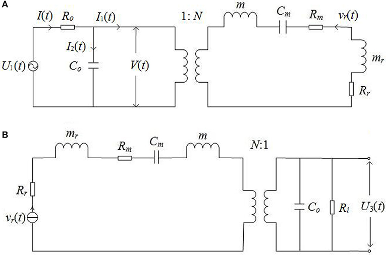
Figure 2. Equivalent circuits of a spherical-shell transducer which is excited by a harmonic sine electric/acoustic signal: (A) source; (B) receiver. U₁(t) is the driving voltage source and R_o is its output resistance; R_i is the input resistance of the measurement circuit; V(t) is the voltage signal at electric-terminals of the source; U₃(t) is the electric-signal at electric-terminals of the receiver; m_r, R_r, C_m, m, C_o, N, and R_m are the radiation mass, radiation resistance, elastic stiffness, mass, clamped capacitance, mechanical–electric conversion coefficient, fraction force resistance of transducer, respectively; and v_r(t) is the vibration velocity at the transducer surface.

FIGURE 3

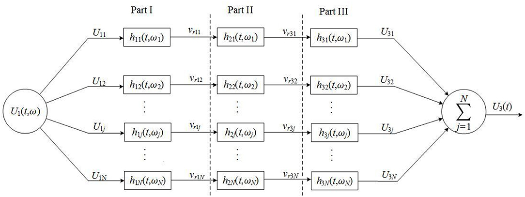
Figure 3. A Schematic representation of a transmission network which shows an acoustic-measurement process. N is the total number of components in frequency spectrum of a driving electric-signal. U_1jis the j^th frequency component in driving electric-signal. v_r1j is the j^th sine frequency component of transducer surface's vibration velocity. v_r3j is the j^th sine frequency component in acoustic-signal arriving at the receiver. U_3j is the j^th frequency component of measured electric-signal created by acoustic-electric conversion of receiver, where j = 1, 2, …, N.

For a spherical thin-shell piezoelectric transducer with harmonic vibration motion, the equations of motion can be solved to establish the corresponding equivalent-circuits as shown in Figure 2.

Applications of residue theorem to the transducer of Figure 2A which is excited by a sine electric-signal, the electric-acoustic impulse response yields potentially the following functional patterns, namely, over-damping, critical-damping and under-damping (oscillatory). And these patterns can be expressed by

$\begin{array}{c}{h}_1(t)=\{\begin{array}{lll}{A}_1\text{exp}\left(-{\alpha }_{1}t\right)+\left[B_1\text{ch}\left(\sqrt{3}Bt\right)+C_1\text{sh}\left(\sqrt{3}Bt\right)\right]\text{exp}\left(-{\beta }_{1}t\right),\hfill & D<0\hfill & \left(1\text{a}\right)\hfill \\ A_2\text{exp}\left(-{\alpha }_{1}t\right)+B_2\text{exp}\left(-{\beta }_{1}t\right)+C_{2}t\text{exp}\left(-{\beta }_{1}t\right),\hfill & D=0\hfill & \left(1\text{b}\right)\hfill \\ A_3\text{exp}\left(-{\alpha }_{1}t\right)+B_3\text{exp}\left(-{\beta }_{1}t\right)\text{cos}\left({\omega }_{1}t+{\phi }_1\right).\hfill & D>0\hfill & \left(1\text{c}\right)\hfill \end{array}\end{array}$

In Equations (1a–c), D is a resultant parameter obtained from the various physical and geometrical parameters of the transducer defined in Supplementary Materials. Practically, the transducer works only with the oscillatory pattern. The derivation of Equations (1a–c) and the various coefficients are given in Supplementary Material Note 1. Similarly, to the transducer in Figure 2B, we have the oscillatory acoustic-electric impulse response

$\begin{array}{rc}{h}_3(t)={Ā}_{3}exp\left[-{\alpha }_{3}t\right]+{\bar{D}}_{3}exp\left[-{\beta }_{3}t\right]cos({\omega }_{3}t+{\phi }_3).& (2)\end{array}$

The derivation of Equation (2) and its various coefficients are presented in Supplementary Material Note 2.

For harmonic vibration of a transducer's surface, two mechanical components (radiation resistance and radiation mass) in the equivalent-circuits shown in either Figures 2A,B are functions of vibration frequency. However, for most cases, either the electric-signal of an exciting source transducer or acoustic-signal arriving at the receiver-transducer is a signal-wavelet with multi-frequency components. Excited by an electric/acoustic signal-wavelet with multi-frequency components, the vibration of the transducer's surface also consists of many sine frequency components.

Because from Fourier transform the electric-signal/acoustic-signal of exciting transducer can be expressed as a linear superposition of sine-wave components with different amplitude, frequency and phase, the electric-acoustic/acoustic-electric excitation process may be represented by a parallel-connected network which consists of many electric-acoustic/acoustic-electric conversion equivalent-circuits as shown by Parts I and III in Figure 3, and each of these equivalent-circuits has its own unique electric-acoustic/acoustic-electric impulse response owing to its distinctive radiation resistance and radiation mass.

A continuous driving electric-signal U₁(t) with amplitude spectrum S(ω)and phase spectrum ϕ(ω) can be decomposed into N frequency components by N-point discrete Fourier transform. Each frequency component can be written as

$\begin{array}{rc}{U}_{1j}(t)=\left|S({\omega }_j)\right|cos\left[{\omega }_{j}t+\varphi ({\omega }_j)\right],& (3)\end{array}$

where j = 1, 2, 3 …… N, |S(ω_j)| and ϕ(ω_j) are the amplitude and the phase of the jth sine frequency component. So, a normalized driving electric-signal is obtained as

$\begin{array}{rc}{U}_1(t)={\displaystyle \sum _{j=1}^N}{U}_{1j}(t)/max\left[\left|{\displaystyle \sum _{j=1}^N}{U}_{1j}(t)\right|\right].& (4)\end{array}$

The output from the jth circuit of Part I in the parallel network (Figure 3) is a convolution of the jth sine frequency component in the driving electric-signal and the jth electric-acoustic impulse response function.

$\begin{array}{rc}{v_{r1j}(t)|}_{{\omega }_j}={\left[U_{1j}{(t)}^{*}{h}_{1j}(t)\right]|}_{{\omega }_j}.& (5)\end{array}$

Then, the normalized vibration speed of the surface of the spherical shell transducer (i.e., radiated acoustic-signal) can be written by

$\begin{array}{cc}{v}_{r1}(t)={\displaystyle \sum _{j=1}^N{v_{r1j}(t)|}_{{\omega }_j}}/\max \left[\left|{\displaystyle \sum _{j=1}^N{v_{r1j}(t)|}_{{\omega }_j}}\right|\right].& (6)\end{array}$

For the jth frequency component of the radiated acoustic-signal, if the propagation medium produces an acoustic impulse response h_2j(t)|_ωj, it would yield the jth frequency component arriving at the receiver.

$\begin{array}{rc}{v}_{r3j}(t,{\omega }_j)={\left[v_{r1j}{(t)}^{*}{h}_{2j}(t)\right]|}_{{\omega }_j,t_{1j}}.& (7)\end{array}$

where, t_1j is the propagation time of the jth sine frequency component from the source to the receiver.

The acoustic-electric conversion of a transducer is an inverse of electric-acoustic conversion. The jth frequency component of an acoustic-signal arriving at the receiver passes the jth circuit (Part III of Figure 3) and is converted to an electric-signal

$\begin{array}{rc}{U}_{3j}(t)={\left[v_{r3j}(t)*h_{3j}(t)\right]|}_{{\omega }_j,t_{1j}}.& (8)\end{array}$

Then, the measured acoustic-signal (i.e., the electric-signal at electric-terminals of the receiver) is a collection of the output from all circuits in Part III of the network (Figure 3), normalized as

$\begin{array}{cc}{U}_3(t)={\displaystyle \sum _{j=1}^N{U}_{3j}(t)}{|}_{{\omega }_j}/\max \left[\left|{\displaystyle \sum _{j=1}^N{U}_{3j}(t)}{|}_{{\omega }_j}\right|\right].& (9)\end{array}$

Now, we can conclude that an acoustic-measurement process can be achieved through the parallel-connected transmission network, as shown in Figure 3.

Transient Process in a Prototype Spherical Shell Transducer

Using piezoelectric material PZT4, we have built two spherical shin-shell transducers polarized in radius direction, whose spherical radius r_b = 7.5 mmand shin-shell thickness l_t = 1.5 mm. The typical physical parameters of PZT4 are ${\epsilon }_{33}^T=130.4186\times {10}^{-10}F/m^2$,$s_{11}^E=12.7\times {10}^{-12}{m}^2/N$, $s_{12}^E=-4.15\times {10}^{-12}{m}^2/N$, $d_{31}=-127\times {10}^{-12}m/V$and ρ = 7.5 × 10³kg/m³[42]. We have also selected water as the medium around the transducer. The density of water ρ_m = 1.000 g/cm³; the propagation velocity of P-wave in water v_m = 1,428.6 m/s.

For a transducer defined in Figure 2, as a source or as a receiver, the calculated parameter D is >0 and the transducer is always in oscillatory mode. Meanwhile, we define a free-mechanical-load transducer as a transducer in vacuum and choose R_r = m_r = R_m = 0. For the cases of mechanical-load, we select the parameter $R_m=0.2\times 4\pi r_b^2{\rho }_m$. And normalized by their corresponding maxima at the free-mechanical-load both the electric-acoustic and the acoustic-electric conversion properties are shown in Figure 4.

FIGURE 4

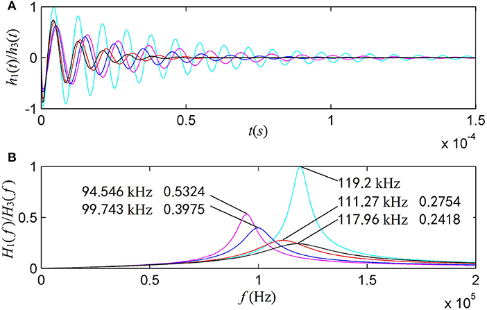
Figure 4. The impulse response and corresponding amplitude spectrum for spherical shell transducer: (A) the impulse response; (B) the amplitude spectrum. The electric-acoustic and acoustic-electric impulse responses and amplitude spectra are normalized by their corresponding maxima for free mechanical-load. The cyan line is the case of free mechanical-load. The other lines are for mechanical-load, where the magenta, blue, red, and black lines stand for the gated sine driving electric-signals with f_s = 0.1, 0.2, 0.5, and 1.5 in unit of f ₁ = 115.0 kHz, respectively.

At the central-frequency 119.2 kHz of the free-loading, both the source and receiver transducers have a maximum transition amplitude which is the largest for all cases. For the mechanical-loaded transducers with harmonic forced-vibrations, a lower forced-vibration frequency corresponds to a lower central-frequency with a larger maximum transition amplitude. With the increased vibration frequency going close to the free-load resonance frequency f ₀, a mechanical-loaded transducer shows a maximum transition-amplitude but it is much smaller than that of the spherical shell transducer free-vibration. These observations confirm that the electric-acoustic/acoustic-electric conversion is dependent not only on the physical and geometrical parameters of a transducer and the physical parameters of the medium around the transducer, but also the forced-harmonic vibration frequency. Understandably, the values of radiation resistance and radiation mass are the function of forced-vibration frequency.

Let's consider a gated sine electric-signal as the source of excitation,

$\begin{array}{rc}{U}_1(t)=\left[H(t)-H(t-t_0)\right]U_{0}sin({\omega }_{s}t).& (10)\end{array}$

where, U₀, ω_s and t₀ are the amplitude, angular frequency, time-window of the driving electric-signal, respectively; and H(·) is Heaviside unit step function. A simple Fourier transform yields the source signal in frequency domain

$\begin{array}{l}{S}_1(\omega )=U_0\{{\omega }_s-({\omega }_s\cos {\omega }_s{t}_0+j\omega \sin {\omega }_s{t}_0)\\ \exp [-j\omega t_0]/({\omega }_s^2-{\omega }^2).& (11)\end{array}$

Now, as an example for the current analysis, we select the source signal parameters U₀ = 1 V, f_s = ω_s/2π = 115.0 kHz and t₀ = 2/f_s. Then, the central frequency of this driving electric-signal is at 110.56 kHz which is slightly smaller than the value of f_s. Figure 5 shows that the theoretical waveform of the driving electric-signal agrees well with the waveform synthesized by discrete Fourier transform, a multidimensional one-way permutation[43]. In turn, it guarantees the accuracy of our following analysis.

FIGURE 5

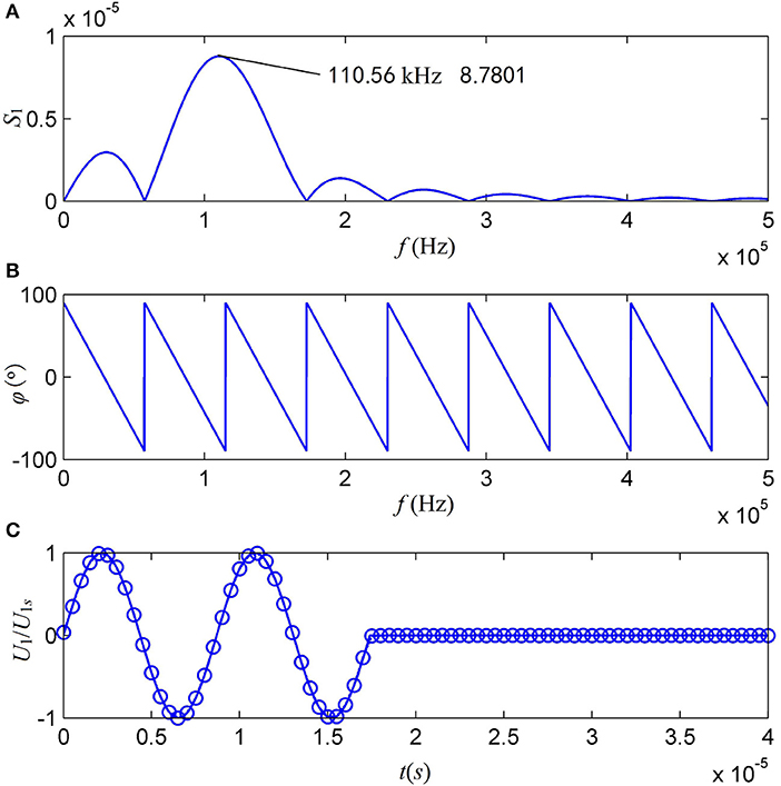
Figure 5. The waveforms of the gated sine driving electric-signal with two cycles and f _s = 115 kHz, where f _s = ω_s/2π. (A) The amplitude spectrum; (B) the phase spectrum; and (C) the waveform. The solid line in (C) is from theoretical calculation and the cycle line is the synthesized waveform from discretized amplitude and phase spectra.

We expanded the gated sine driving electric-signal as a series of sine-waves with different frequency, amplitude and phase. Applying each of these sine-components as an individual excitation source for the parallel circuits of Figure 3, we obtained an output signal from each parallel circuit in this network. The results of calculations from Equation 5 are very revealing (Figure 6). Figures 6A–D are the acoustic-signals radiated from the source transducer when it is excited by several selected sine-components, showing that for each circuit in the network, the transient response has a brief transition period right after the excitation followed by a regular sine-vibration with a corresponding frequency. The cumulative output of all parallel circuits in Part I of Figure 3 forms the vibration velocity on the surface of the spherical shell transducer, which is given by the black-curve in Figure 6E. The corresponding amplitude spectrum is given by the black-curve in Figure 6F, showing that the central frequency of the radiated acoustic-signal is 115.83 kHz which is smaller than the free-load central frequency 119.2 kHz and larger than that of gated sine driving electric-signal at 110.56 kHz. We choose a theoretical model of assumed acoustic-source in previous published literature, Tsang wavelet, as an example to perform comparison with the parallel-connected equivalent-circuit model proposed by us. The expressions of Tsang wavelet in time and frequency domains [25] are

$\begin{array}{rc}x(t)=4\alpha texp\left[-\alpha t\right]sin({\omega }_{0}t)H(t),& (12)\end{array}$

$\begin{array}{rc}X(f)=\frac{8\alpha {\omega }_0(\alpha -j\omega )}{\left[{(\alpha -j\omega )}^2+{({\omega }_0)}^2\right]},& (13)\end{array}$

where α is a damping coefficient, ω₀ = 2πf₀ andω = 2πf.

FIGURE 6

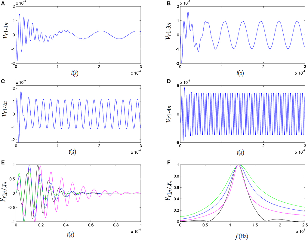
Figure 6. The convolution of the gated sine driving electric-signal with the electric-acoustic impulse response from the parallel connected network of a spherical shin-shell transducer as well as the waveform and amplitude spectrum of Tsang wavelet: (A–D) are the convolutions of selected frequency components of electric driving-signal with corresponding electric-acoustic impulse response at f_i = 0.1f ₁, 0.2f ₁, 0.5f ₁, and 1.5f ₁, where f ₁ = 115 kHz and t₀ = 2/f _1; (E) is the normalized waveforms, which are a cumulative convolution of all frequency components in the network, and those of Tsang wavelet; (F) is the normalized amplitude spectrum of our transducer's transient response model and the amplitude spectra of Tsang wavelet.

Let f₀(= ω₀/2π) be equal to 115.76 kHz and α be equal to 0.3ω₀/π, 0.5ω₀/π and 0.7ω₀/π, the waveforms and amplitude spectra of Tsang wavelet are calculated as shown by magenta, green and blue curves in Figure 6, respectively. The larger the value of α is, the shorter the waveform duration of Tsang wavelet is and the narrower its amplitude spectrum is. There are some apparent differences between the waveform and amplitude spectrum of Tsang wavelet and those of our model (black curves) in Figure 6. The head-wave amplitudes of Tsang wavelet are greater than that of our model, and it has more low/high frequency components compared to our model.

The acoustic-signal radiated from the studied source transducer is spherical. If we assume that water is an ideal elastic medium, then the acoustic-signal propagating inside the water could have potentially geometrical attenuation but not viscous attenuation. Additionally, all frequency components of the acoustic-signal would propagate in the same speed; the shapes of the waveform and frequency spectrum would not change; and the amplitude would decrease with respect to the increased propagation distance only. Under these conditions, we are interested to find only the signals at the electric-terminals of the receiver-transducer. The acoustic impulse response of water can then be written as

$\begin{array}{rc}{h}_2(t)=\delta (t-t_1)/(1+r),& (14)\end{array}$

where, h₂₁(t, ω₁) = … = h_2j(t, ω_j) = …h_2N(t, ω_N) = h₂(t), t₁ and r are the propagation time and distance of the radiated signal in water. To determine the quality of a transducer on electric-acoustic/acoustic-electric conversion, one of the most important piece of information comes from the analysis of the output signal after electric-acoustic transduction. To accomplish this operation, we set a distance from the source-transducer to the receiver-transducer at 0.73 m. Applying the gated-sine driving electric-signal to the source-transducer, we have calculated the cumulative output signals on the receiver-transducer. Figures 7A–D show the convoluted signals at the receiver-transducer (Part III of Figure 3) from a few selected frequency components in the acoustic-signal arriving at the receiver-transducer. Again, the transient response has a brief transition period initial excitation followed by a regular sine-vibration with a corresponding frequency.

FIGURE 7

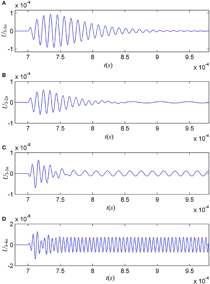
Figure 7. The convoluted signals at the receiver (Part III of Figure 3) from several selected sine frequency components. (A–D) are the cases of f_i = 0.1f ₁, 0.2f ₁, 0.5f ₁, and 1.5f ₁, respectively.

Figure 8 shows the cumulative signals of waveform and amplitude spectrum at the electric-terminals of the transducer, in comparison to the experimental observation from the theoretical model. Comparing the calculated results of the theoretical model with the measured acoustic-signal at the electric-terminals of the receiver-transducer, it shows that the measured signal has a slightly larger time window and its central frequency is 115.76 kHz, which is slightly lower than that (116.47 kHz) obtained from calculation. Meanwhile, comparing to the acoustic-signal radiated by the source-transducer from theoretical calculation, we also can see that the signals at the receiver-transducer's electric-terminals from theoretical calculation and measurement have slightly larger time windows and the widths of their amplitude spectra become slightly narrower. However, the central frequency (115.76 kHz) of the measured acoustic-signal is slightly lower than that of the acoustic-signal radiated by the source transducer (115.83 kHz) from theoretical calculation. We believe that this is caused by so called acoustic-electric filtering effect of the transducer. Through acoustic-electric filtering inside the transducer, the frequency components of the signal far away from the transducer' central frequency (near to 116.67 kHz) are filtered or strongly oppressed.

FIGURE 8

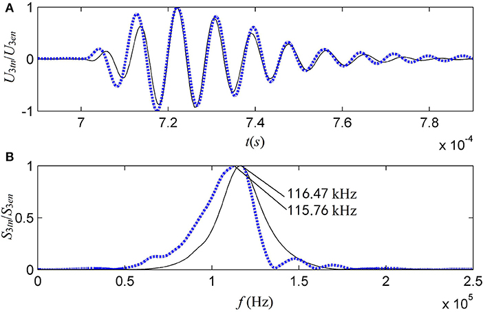
Figure 8. Normalized electric-signals at the receiver-transducer (Part III of Figure 3). The solid lines are from the theoretical model and the dotted-lines are from experimental measurement. (A) Waveform. (B) Amplitude spectrum.

As an alternative test for the newly proposed model in this paper, we have calculated the frequencies corresponding to the main peaks of amplitude spectra of both the acoustic-signal radiated at the source transducer and the electric-signal at the receiver-transducer as a function of gated-sine driving electric-signal's frequency (f_s). These relationships are compared to the data from our experimental measurement, shown in Figure 9.

FIGURE 9

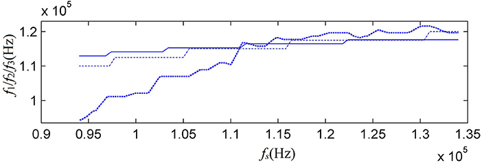
Figure 9. The relationship between the frequency (f_s) of the gated driving sine-electric-signal and the main-peak frequencies of amplitude spectra for radiated and measured acoustic-signals: dash-dot line is the calculated acoustic-signal radiated at the source-transducer's mechanical-terminals; solid line is the calculated electric-signal at receiver-transducer's electric-terminals; and dotted line is the experimentally measured electric-signal at receiver-transducer's electric-terminals.

The above calculated results show that the waveform and frequency spectrum of the radiated acoustic-signal are determined by both the property of the electric-acoustic conversion and that of the driving electric-signal. For a given transducer, the radiated acoustic-signal varies with the driving electric-signal.

Disucussion

To confirm the rationality of the newly proposed transient response model of the transducer, we have developed an experimental measurement system specially, which consists of a mechanical assembly, an electrical hardware module, and a system software module aimed at control and computation and its structure-flowchart is shown Figure 10. The mechanical assembly includes steering-engines, stepping motors, sliding rails, and a silencing tank. The electrical-hardware comprises a computer for graphic interface, an electric-signal waveform generator, a power amplifier and a microcontroller which is used to control the space position and direction of source/receiver, a digitizer with 16–24 bit and 5–15 MHz sampling rate and a desktop. For so high resolution and sampling rate, the system can guarantee accurate measurement of experimental verification.

FIGURE 10

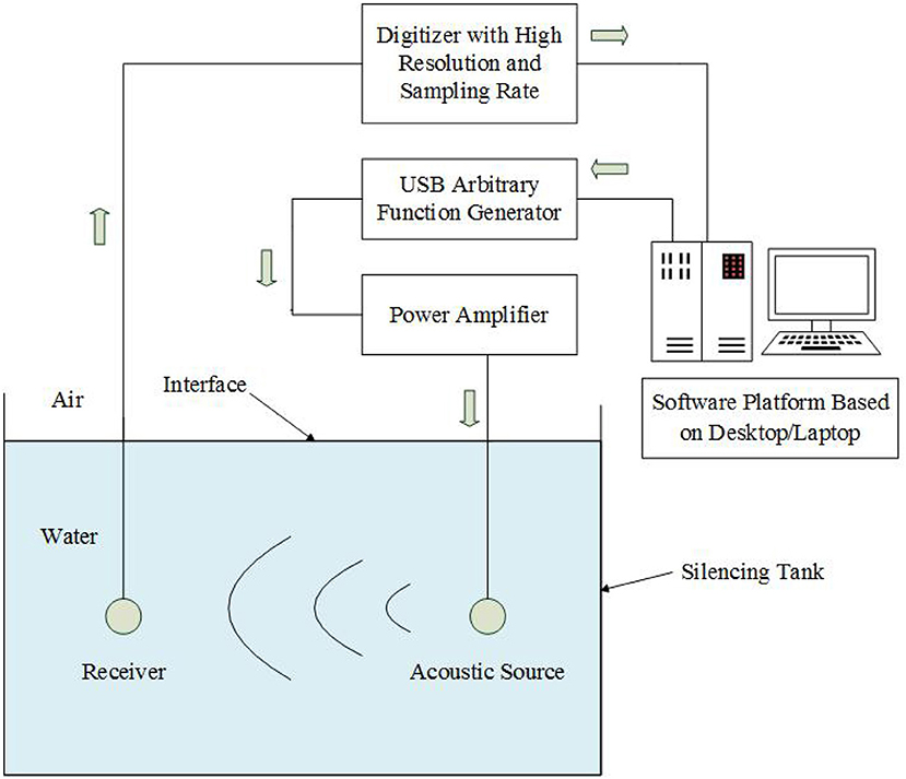
Figure 10. Block diagram of experimental measurement system.

We also specially fabricated two spherical shin-shell transducers with piezoelectric material PZT4, polarized in radius direction, whose inner spherical radius and thickness are 7.5 mm and 1.5 mm, respectively. The physical and mechanical parameters of the two spherical shell transducers are the same as those used in the calculations. We put them in a silencing tank fulled with water for experimental measurement. We also set two transducers in water, separated by a distance of 0.73 m. One transducer was used as source and another one was used as receiver.

During experimental measurement, the desktop sends a command to the waveform generator and make it create a gated sine electric-signal with two cycles and f _s = 115 kHz. By power amplification, the gated sine electric-signal provided excitation to the source transducer to emit acoustic-signal. The radiated acoustic-signal propagated to the receiver through water as the medium and then was converted to the electric-signal which was acquired by the digitizer and provided feed-back to the desktop computer control central. By using this system we obtain the transient responses of a realistic spherical shell PZT transducer polarized in radius direction.

The waveform and amplitude spectrum of the electric-signal at receiver-transducer's electric-terminals were measured and compared to the theoretical calculation based on the newly proposed model, as given in Figure 8. The frequency corresponding to the amplitude spectrum's main-peak varies with the frequency f _s of the gated sine electric-signal. The measured relationship between them was given in Figure 9, also provided a comparison between the theoretical calculations and the experimental observation. From Figure 8 we find that the acoustic-signal waveform (at the receiver's electrical terminals) from the theoretical calculation is very similar to that from experimental measurement and this fact shows that our model of source-transducer's transient-response is more closed to practical case compared to the assumed Tsang wavelet model. The central frequency of the calculated acoustic-signal at the electric-terminals is 116.47 kHz and that of the measured acoustic-signal is 115.76 kHz. The frequency corresponding to amplitude spectrum's main-peak in Figure 8B varies with the frequency f_s of the gated sine electric-signal and the relationship between them is measured as shown as the dotted-curve in Figure 9. It is worth noting that when the frequency of the gated sine electric-signal is far away the central-frequency of the transducer, the value of this main-peak can be smaller than that of sub-peak for the amplitude spectrum curves. So, a good agreement between theoretical calculation and experimental measurement has been achieved.

By the modeling, calculations and experimental measurements, we have a further understanding for the transient responses of the electric-acoustic/acoustic-electric conversions of the piezoelectric transducer. (i) For the spherical shell transducer in theory, there are three states of either electric-acoustic conversion or acoustic-electric conversion: overdamped, critically damped and oscillatory mode. However, only the last mode is of practical application. (ii) The electric-acoustic conversion property of the transducer is reciprocal to its acoustic-electric conversion property. (iii) In the practical application of the transducer, either the driving electric-signal of inputting to the transducer's electric-terminals or the acoustic-signal of inputting to its mechanical-terminals contains a lot of frequency components. Because the two mechanic elements (radiation resistance and radiation mass) in the transducer's equivalent-circuit are functions of the frequency and the equivalent-circuit is established from the harmonic vibration status of the transducer, the acoustic measurement process can be viewed as a signal transmission system with many parallel-connected equivalent-circuits. (iv) The properties of the electric-acoustic/acoustic-electric conversions of the transducer (including its impulse response, amplitude spectrum and central- frequency) are not only determined by the physical and geometrical parameters of the transducer and the physical parameters of the medium around the transducer, but also by the property and type of the driving electric-signal. (v) Except for the property of propagation medium, the properties of the measured acoustic-signal in time and frequency domains also depend on the electric-acoustic/electric-electric conversion property and the properties of driving electric-signal. (vi) Comparing to the assumed acoustic-source models as reported in the literatures, e.g., Tsang wavelet, the new model of the transducer's transient response proposed in this paper is more realistic in practical applications.

Data Availability Statement

The data that support the findings of this study are available from the corresponding author upon reasonable request.

Author Contributions

LF and MZ designed the project and performed theory derivation. YF designed the experiment device. XZ, YZ, HY, ST, and GL performed theoretical calculations. ML, PD, and JM developed the experimental device. QZ and MW performed experimental measurements and analysis.

Conflict of Interest Statement

The authors declare that the research was conducted in the absence of any commercial or financial relationships that could be construed as a potential conflict of interest.

Acknowledgments

This work is supported by Xi'an University of Posts and Telecommunications and by the Physical Sciences Division at The University of Chicago.

Supplementary Material

The Supplementary Material for this article can be found online at: https://www.frontiersin.org/articles/10.3389/fphy.2018.00123/full#supplementary-material

References

1. Wu J, Fedder GK, Carley LR. A low-noise low-offset capacitive sensing amplifier for a 50-$\mu g/\sqrt{Hz}$ monolithic CMOS MEMS accelerometer. IEEE J Solid State Circuits (2004) 39:722–30. doi: 10.1109/JSSC.2004.826329

CrossRef Full Text | Google Scholar

2. Xie J, Lee C, Feng H. Design, fabrication, and characterization of CMOS MEMS-based thermoelectric power generators. J Micromech Syst. (2010) 19:317–24. doi: 10.1109/JMEMS.2010.2041035

CrossRef Full Text | Google Scholar

3. Fa L, Zhao J, Han YL, Li GH, Ding PF, Zhao MS. The influence of rock anisotropy on elliptical-polarization state of inhomogenously refracted P-wave. Sci China Phys Mech Astron. (2016) 59:644301. doi: 10.1007/S11433-015-00441-1

CrossRef Full Text | Google Scholar

4. Fa L, Castagna JP, Suarez-Rivera R, Sun P. An acoustic-logging transmission-network model (continued): addition and multiplication ALTNs. J Acoust Soc Am. (2003) 113:2698–073. doi: 10.1121/1.1562651

PubMed Abstract | CrossRef Full Text | Google Scholar

5. Gubbi J, Buyya R, Palaniswami MS. Internet of Things (IoT): A vision, architectural elements, and future directions. Future Gener Comput Syst. (2013) 29:1645–60. doi: 10.1016/j.future.2013.01.010

CrossRef Full Text | Google Scholar

6. Tadigadapa S, Mateti K. Piezoelectric MEMS sensors: state-of-the-art and perspectives Meas. Sci Technol. (2009) 20:092001. doi: 10.1088/0957-0233/20/9/092001

CrossRef Full Text | Google Scholar

7. Dausch DE, Gilchrist KH, Carlson JB, Hall SD, Castellucci JB, von Ramm OT. In vivo realtime 3-D intracardiac echo using PMUT arrays. IEEE Trans Ultrason Ferroelect Freq Control (2014) 61:1754–64. doi: 10.1109/TUFFC.2014.006452

CrossRef Full Text | Google Scholar

8. Goh AS, Kohn JC, Rootman DB, Lin JL, Goldberg RA. Hyaluronic acid gel distribution pattern in periocular area with high-resolution ultrasound imaging. Aesthetic Surg J. (2014) 34:510–5. doi: 10.1177/1090820X14528206

PubMed Abstract | CrossRef Full Text | Google Scholar

9. Przybyla RJ, Tang HY, Guedes A, Shelton SE, Horsley DA, Boser BE. 3D ultrasonic rangefinder on a chip. IEEE J Solid State Circuits (2015) 50:320–34. doi: 10.1109/JSSC.2014.2364975

CrossRef Full Text | Google Scholar

10. Lu Y, Tang H, Fung S, Wang Q, Tsai J, Daneman M, et al. Ultrasonic fingerprint sensor using a piezoelectric micromachined ultrasonic transducer array integrated with complementary metal oxide semiconductor electronics. Appl Phys Lett. (2015) 106:263503. doi: 10.1063/1.4922915

CrossRef Full Text | Google Scholar

11. He Q, Liu J, Yang B, Wang X, Chen X, Yang C. MEMS-based ultrasonic transducer as the receiver for wireless power supply of the implantable microdevices. Sens Actuators A Phys. (2014) 219:65–72. doi: 10.1016/j.sna.2014.07.008

CrossRef Full Text | Google Scholar

12. Breazeale MA, Adler L, Scott GW. Interaction of ultrasonic waves incident at the Rayleigh angle onto a liquid-solid interface. J Appl Phys. (1977) 48:530–7. doi: 10.1063/1.323677

CrossRef Full Text | Google Scholar

13. Atlar A, Quate CF, Wickramasinghe HK. Phase imaging in reflection with the acoustic microscope. Appl Phys Lett. (1977) 31:791–3. doi: 10.1063/1.89551

CrossRef Full Text | Google Scholar

14. Briers R, Leroy O, Shkerdin G. Bounded beam interaction with thin inclusions. Characterization by phase differences at Rayleigh angle incidence. J Acoust Soc Am. (2000) 108:1622–30. doi: 10.1121/1.1289364

PubMed Abstract | CrossRef Full Text | Google Scholar

15. Ranjith PG, Jasinge D, Song JY, Choi SK. A study of the effect of displacement rate and moisture content on the mechanical properties of concrete: use of acoustic emission. Mech. Mater (2008) 40:453–69. doi: 10.1016/j.mechmat.2007.11.002

CrossRef Full Text | Google Scholar

16. Scruby CB. An introduction to acoustic emission. J Phys E (1987) 20:945–53.

Google Scholar

17. Elfergani HA, Pullin R, Holford KM. Damage assessment of corrosion in prestressed concrete by acoustic emission. Constr Build Mater (2013) 40:925–33. doi: 10.1016/j.conbuildmat.2012.11.071

CrossRef Full Text | Google Scholar

18. Behrens BA, Bouguecha A, Buse C, Wölki K, Santangelo A. Potentials of in situ monitoring of aluminum alloy forging by acoustic emission. Arch Civ Mech Eng. (2016) 16:724–33. doi: 10.1016/j.acme.2016.04.012

CrossRef Full Text | Google Scholar

19. Bhuiyan MSH, Choudhury IA, Dahari M, Nukman Y, Dawal SZ. Application of acoustic emission sensor to investigate the frequency of tool wear and plastic deformation in tool condition monitoring. Measurement (2016) 92:208–17. doi: 10.1016/j.measurement.2016.06.006

CrossRef Full Text | Google Scholar

20. Girard L, Gruber S, Weber S, Beutel J. Environmental controls of frost cracking revealed through in situ acoustic emission measurements in steep bedrock. Geophys Res Lett. (2013) 40:1748–53. doi: 10.1002/grl.50384

CrossRef Full Text | Google Scholar

21. Li D, Du F. Monitoring and evaluating the failure behavior of ice structure using the acoustic emission technique. Cold Reg Sci Technol. (2016) 129:51–9. doi: 10.1016/j.coldregions.2016.06.003

CrossRef Full Text | Google Scholar

22. Moradian Z, Einstein HH, Ballivy G. Detection of cracking levels in brittle rocks by parametric analysis of the acoustic emission signals. Rock Mech Rock Eng. (2015) 49:785–800. doi: 10.1007/s00603-015-0775-1

CrossRef Full Text | Google Scholar

23. Arnau A. Piezoelectric Transducers and Applications. Berlin: Springer (2008).

Google Scholar

24. Ricker N. Wavelet contraction,wavelet expansion,and the control of seismic resolution. Geophysics (1953) 18:769–92. doi: 10.1190/1.1437927

CrossRef Full Text | Google Scholar

25. Tsang L, Rader D. Numerical evaluation of the transient acoustic waveform due to a point source in a fluid-filled borehole. Geophysics (1979) 44:1706–20. doi: 10.1190/1.1440932

CrossRef Full Text | Google Scholar

26. Cheng C, Toksöz MN. Elastic wave propagation in a fluid filled borehole and synthetic acoustic logs. Geophysics (1981) 46:1042–53.

Google Scholar

27. Tubman KM, Cheng CH, Toksoz MN. Synthetic full waveform acoustic logs in cased boreholes. Geophysics (1984) 49:1051–9. doi: 10.1190/1.1441720

CrossRef Full Text | Google Scholar

28. Kurkjian AL. Numerical computation of individual far-field arrivals excited by an acoustic source in a borehole. Geophysics (1985) 50:852–66. doi: 10.1190/1.1441961

CrossRef Full Text | Google Scholar

29. Stephen RA, Cardo-Casas F, Cheng CH. Finite-difference synthetic acoustic logs. Geophysics (1985) 50:1588–609. doi: 10.1190/1.1441849

CrossRef Full Text | Google Scholar

30. Schmitt DP, Bouchou M, Bonnet J. Full-wave synthetic logs in radially semiinfinite saturated porous media. Geophysics (1988) 53:807–23. doi: 10.1190/1.1442516

CrossRef Full Text | Google Scholar

31. Renlie L. Effect of a soft layer on the normal models in a fluid-filled borehole. J Acoust Soc Am. (1993) 94:2963. doi: 10.1121/1.407327

CrossRef Full Text | Google Scholar

32. Renlie L, Raaen AM. Sonic wave propagation in fluid filled borehole surrounded by a formation with trees relief induced anisotropy. Geophysics (1993) 58:1257–69. doi: 10.1190/1.1443509

CrossRef Full Text | Google Scholar

33. Kostek S, Randall CJ. Modeling of a piezoelectric transducer and its application to full waveform acoustic logging. J Acoust Soc Am. (1994) 95:109–22. doi: 10.1121/1.408368

CrossRef Full Text | Google Scholar

34. Richard L, Gibson J. Radiation from seismic sources in cased and cemented boreholes. Geophysics (1994) 59:518–33. doi: 10.1190/1.1443613

CrossRef Full Text | Google Scholar

35. Gibson RL, Peng C. Low- and high-frequency radiation from seismic sources in cased boreholes. Geophysics (1994) 59:1780–5. doi: 10.1190/1.1443565

CrossRef Full Text | Google Scholar

36. Sheriff RE, Geldart LP. Exploration Seismology. New York, NY: Cambridge University Press (1995).

Google Scholar

37. Liu L, Lin WJ, Zhang HL, Wang XM. A numerical investigation of the acoustic mode waves in a deviated borehole penetrating a transversely isotropic formation. Sci China-Phys Mech Astron (2015) 58:08430. doi: 10.1007/s11433-015-5678-3

CrossRef Full Text | Google Scholar

38. Zhang XM, Wang XM, Zhang HL. Leaky modes and the first arrivals in cased boreholes with poorly bonded conditions. Sci China Phys Mech Astron. (2016) 59:624301. doi: 10.1007/s11433-015-5756-6

CrossRef Full Text | Google Scholar

39. Fa L, Xue L, Fa YX, Han YL, Zhang YD, Cheng HS, et al. Acoustic goos-hänchen effect. Sci China Phys Mech Astron. (2017) 60:104311. doi: 10.1007/s11433-017-9052-9

CrossRef Full Text | Google Scholar

40. Piquette JC. Method for transducer suppression. I: theory. J Acoust Soc Am. (1992) 92:1203–13.

Google Scholar

41. Piquette JC. Method for transducer suppression. II: experiment. J Acoust Soc Am. (1992) 92:1214–21.

42. Fa L, Castagna JP, Hovem JM. “Derivation and simulation of source function for acoustic logging.” in Proceedings of the IEEE Ultrasonics Symposium. Lake Tahoe, NV (1999) 1:707–10.

Google Scholar

43. de Castro A. Quantum one-way permutation over the finite field of two elements. Quant Inform Process. (2017) 16:149. doi: 10.1007/s11128-017-1599-6

CrossRef Full Text | Google Scholar