Optical Solitons With M-Truncated and Beta Derivatives in Nonlinear Optics

1. Introduction

Nonlinearity has been potent field of research and its vitality is thought of through a sweer-amplitude wave oscillation analyzed in numerous fields from plasmas and fluids to biological and chemical phenomenon, solid state, to mention a few. Therefore, the most captivating viewpoint in nonlinear physical phenomenon are solitons. The availability of solitonic concepts are due to the philosophical balance of dispersion and nonlinearity [1]. A lot of researches on solitons and associated aspects of solitary wave (SW) solutions for example monopulse water wave which depict the first soliton can be found in Miller and Ross [2], Podlubny [3], Oldham [4], Kiryakova [5], and El-Sayed and Gaber [6]. Moreover, various mathematical insight and modeling can be interpreted through optical solitons for their numerical and analytical structures of the numerous mechanism. These stimulated many engineers and scientists to focus on the establishments of solitons with optical structures with the help of various integration schemes [7–38].

For quite a long time, the effect of memory is an idea that has been of great concern in the locality of modeling. Genuinely, the integer systems are not conveniently addressing this memory effect [39–41]. Many researchers have presented that, one can get to know more on the memory effect through non-integer operators [42–45]. An extension to integer order systems such as conformable [46], beta [47], and M-derivatives [48] have also been introduced and they play a vital role in modeling physical systems. These extension to integer order systems satisfy a lot of characteristics that were not satisfied before and it can be employed to model several physical phenomenon. In this study, we establish new optical solitons for the governing equation with M-truncated and beta derivatives with the aid of two well-known method. The M-truncated and beta derivatives are defined in the following subsections, respectively.

1.1. Truncated M-Fractional Derivative

We define the truncated Mittag-Leffler function of one parameter by

$\begin{array}{ll}{{}_{i}E}_{\beta }(z)={\displaystyle \sum _{k=0}^i\frac{z^k}{\Gamma (\beta k+1)}}.& (1)\end{array}$

Truncated M-fractional derivative (TMD) is a fractional derivative that has been introduced in Sousa and de Oliveira [48]. This derivative has expunged the obstacles with the existing derivatives. It is defined in the following definition.

Definition 1.1. Assume that f : (0, ∞) → ℝ, the TMD of f with order γ exhibited ${{}_{i}T}_M^{\gamma ,\beta }$ is given by

$\begin{array}{ll}{{}_{i}T}_M^{\gamma ,\beta }f(\tau )=\underset{ϵ\to 0}{\lim }\frac{f\left(\tau {+}_i{E}_{\beta }\right(ϵ{\tau }^{-\gamma }\left)\right)-f(\tau )}{ϵ},& (2)\end{array}$

for τ > 0, and _iE_βγ ∈ (0, 1), β > 0 is a truncated Mittag-Leffler function of one parameter, as defined in (1). Note that, if f is γ-differentiable in some open interval (0, a), a > 0, and ${\lim }_{\tau \to 0^{+}}\left(i{T}_M^{\gamma ,\beta }f(\tau )\right)$. Then we attain

$\begin{array}{ll}{{}_{i}T}_M^{\gamma ,\beta }f(0)=\underset{\tau \to 0^{+}}{\lim }\left({{}_{i}T}_M^{\gamma ,\beta }f(\tau )\right)& (3)\end{array}$

Theorem 1.1. Surmise that f : (0, ∞) → ℝ is γ−differentiable for τ₀ > 0, with γ ∈ (0, 1], β > 0, then f is continuous at τ₀.

Theorem 1.2. Let 0 < γ ≤ 1, β > 0, a, b ∈ ℝ, f, g, γ-differentiable, at a point τ > 0. Then

• ${{}_{i}T}_M^{\gamma ,\beta }(af+bg)=a_i{T}_M^{\gamma ,\beta }(f)+b_i{T}_M^{\gamma ,\beta }(f)$, a, b ∈ ℝ

• ${{}_{i}T}_M^{\gamma ,\beta }(t^{\mu })=\mu {\tau }^{\mu -\gamma }$, μ ∈ ℝ

• ${{}_{i}T}_M^{\gamma ,\beta }(fg)=f_i{T}_M^{\gamma ,\beta }(g)+g_i{T}_M^{\gamma ,\beta }(f)$,

• ${{}_{i}T}_M^{\gamma ,\beta }(\frac{f}{g})=\frac{g_i{T}_M^{\gamma ,\beta }(f)-f_i{T}_M^{\gamma ,\beta }(g)}{g^2}$,

• If f is differentiable, then ${{}_{i}T}_M^{\gamma ,\beta }(f)(\tau )=\frac{{\tau }^{1-\gamma }}{\Gamma (\beta +1)}\frac{df}{d\tau }$,

• ${{}_{i}T}_M^{\gamma ,\beta }(fog)(\tau )=f^{\prime }{(g(\tau ))}_i{T}_M^{\gamma ,\beta }g(\tau )$, for f differentiable at g.

1.2. Beta Derivative

The beta derivative can be stated by [49]

$\begin{array}{ll}{{}_0{}^{A}T}_{\eta }^{\gamma }(F(\eta ))=\underset{ϵ\to 0}{\lim }\frac{F\left(\eta +ϵ(\eta +\frac{1}{\Gamma (\gamma )})\right)-F(\eta )}{ϵ}.& (4)\end{array}$

along with the properties as comes next

1.

$\begin{array}{ll}{{}_0{}^{A}T}_{\eta }^{\gamma }(aF(\eta )+bG(\eta ))=a_0^A{T}_{\eta }^{\gamma }F(\eta )+b_0^A{F}_{\eta }^{\gamma }G{(\eta )}_0^A& (5)\end{array}$

2.

$\begin{array}{ll}{T}_{\eta }^{\gamma }(c)=0,& (6)\end{array}$

for any c depicting a constant,

3.

$\begin{array}{ll}{{}_0{}^{A}T}_{\eta }^{\gamma }(F(\eta ).G(\eta ))=G{(\eta )}_0^A{T}_{\eta }^{\gamma }F(\eta )+F{(\eta )}_0^A{T}_{\eta }^{\gamma }G(\eta )& (7)\end{array}$

4.

$\begin{array}{ll}{{}_0{}^{A}T}_{\eta }^{\gamma }\left(\frac{F(\eta )}{G(\eta )}\right)=\frac{G{(\eta )}_0^A{T}_{\eta }^{\gamma }F(\eta )-F{(\eta )}_0^A{T}_{\eta }^{\gamma }G(\eta )}{G^2(\eta )}.& (8)\end{array}$

Considering $ϵ={\left(\eta +\frac{1}{\Gamma (\gamma )}\right)}^{\gamma -1}h$, h → 0 when ϵ → 0, therefore we have

$\begin{array}{ll}{{}_0{}^{A}T}_{\eta }^{\gamma }F(\eta )={\left(\eta +\frac{1}{\Gamma (\gamma )}\right)}^{1-\gamma }\frac{dF(\eta )}{d\eta },& (9)\end{array}$

with

$\begin{array}{ll}\xi =\frac{l}{\gamma }{\left(\eta +\frac{1}{\Gamma (\gamma )}\right)}^{\gamma }& (10)\end{array}$

where l is a constant.

5.

$\begin{array}{ll}{{}_0{}^{A}T}_{\eta }^{\gamma }\left(\frac{F(\tau )}{G(\eta )}\right)=l\frac{dF(\tau )}{d\tau }.& (11)\end{array}$

The arrangements of the paper is as follows: In section 2 the governing equation has been presented. In section 3, applications have been reported, whereas section 4 provides the discussion of the obtained results along with their physical features. Finally, concluding remark is given in section 5.

2. Governing Equation

The CGLE equation [50, 51] in the sense of M-truncated derivative is given by:

$\begin{array}{r}\hfill i_0^E{{D}}_{M,\tau }^{\gamma ,\beta }u+a_0^E{{D}}_{M,\eta }^{2\gamma ,\beta }u+b\mathbb{F}(|u{|}^2)u\\ \hfill =\frac{1}{|u{|}^2{u}^{*}}\{{\delta }_0^E{{D}}_{M,\eta }^{2\gamma ,\beta }(|u{|}^2)|u{|}^2-B{{(}_0^E{{D}}_{M,\eta }^{\gamma ,\beta }u)}^2\}+Au,& (12)\end{array}$

whereas in the sense of beta derivative is given by

$\begin{array}{r}\hfill i_0^E{{D}}_t^{\gamma }u+a_0^E{{D}}_{\eta }^{2\gamma }u+b\mathbb{F}(|u{|}^2)u\\ \hfill =\frac{1}{|u{|}^2{u}^{*}}\{{\delta }_0^E{{D}}_{\eta }^{2\gamma }(|u{|}^2)|u{|}^2-B{{(}_0^E{{D}}_{\eta }^{\gamma }u)}^2\}+Au,& (13)\end{array}$

where ${{}_o{}^E{D}}_{M,\tau }^{\gamma ,\beta }$, ${{}_o{}^E{D}}_{M,\eta }^{\gamma ,\beta }$, and ${{}_o{}^E{D}}_{\tau }^{\gamma }$, ${{}_o{}^E{D}}_{\tau }^{\gamma }$ depicts M-truncated and beta derivatives, respectively. 0 < γ ≤ 1, describing the order of the fractional derivatives and a, b, δ, B, and A are real constants.

In Equations (12) and (13), 𝔽 ∈ ℝ, and the complex function and its smoothness is necessary to be possessed 𝔽(|u|²)u : ℂ → ℂ. Consider ℂ to be a two-dimensional linear space ℝ², and that 𝔽(|u|²)u is k times continuously differentiable, so that

$F(|u{|}^2)u\in {\displaystyle \bigcup _{m,n=1}^{\infty }}{c}^k((-n,n)\times (-m,m);{ℝ}^2).$

2.1. Mathematical Analysis

To solve Equations (12) and (13), the beginning step is as come next

$\begin{array}{ll}u(\eta ,\tau )=u(\xi )e^{i\varphi (\eta ,\tau )},& (14)\end{array}$

the shape of the pulse is represented by u(η, τ) so that in the sense of M-truncated derivatives we have

$\begin{array}{ll}\xi =\frac{\Gamma (\beta +1)}{\gamma }({\eta }^{\gamma }-\upsilon {\tau }^{\gamma })& (15)\end{array}$

and

$\begin{array}{ll}\varphi (\eta ,\tau )=-\frac{\Gamma (\beta +1)}{\gamma }(k{\eta }^{\gamma }-w\upsilon {\tau }^{\gamma })+{\theta }_0(\xi ),& (16)\end{array}$

and in the sense of beta derivative we have

$\begin{array}{ll}\xi =\frac{1}{\gamma }{\left(\eta +\frac{1}{\Gamma (\gamma )}\right)}^{\gamma }-\frac{\upsilon }{\gamma }{\left(\tau +\frac{1}{\Gamma (\gamma )}\right)}^{\gamma }& (17)\end{array}$

and

$\begin{array}{ll}\varphi (\eta ,\tau )=-\frac{k}{\gamma }{\left(\eta +\frac{1}{\Gamma (\gamma )}\right)}^{\gamma }+\frac{w}{\gamma }{\left(\tau +\frac{1}{\Gamma (\gamma )}\right)}^{\gamma }+{\theta }_0(\xi ),& (18)\end{array}$

where w is the wave number of the soliton, k denotes the soliton frequency, υ indicates the speed of the soliton, ϕ(η, τ) is the phase component, θ₀(ξ) depicts an additional phase function depending on ξ. Plugging (15) and (17) into (12) and (13), respectively, and decomposing the real and imaginary parts, one attains

$\begin{array}{ll}wu+a(u^{″}-k^{2}u)+b{F}(u^2)u=2(\delta -2B)\frac{u^{\prime 2}}{u}+2\delta u^{″}+Au,& (19)\end{array}$

and

$\begin{array}{ll}\upsilon =-2ak.& (20)\end{array}$

Equation (20) denotes the soliton velocity. Setting δ = 2B in Equation (19) yields.

$\begin{array}{ll}(a-4B)u^{″}-(w+a{k}^2+A)u+b{F}(u^2)u=0.& (21)\end{array}$

2.2. Kerr Law

This law has got its origin through the reality that a light wave in an optical fiber heads to responses by a nonlinear patterns from non-harmonic motion of electrons bound in molecules, brought externally by an electric field. Although the responses by nonlinear terms are seriously low, over a long distance of propagation, the effects standstill in numerous patterns measuring in terms of light wavelength. This law is given by ${F}(u)=u$, therefore Equation (21) becomes.

$\begin{array}{ll}(a-4B)u^{″}-(w+a{k}^2+A)u+b{u}^3=0.& (22)\end{array}$

3. Applications

This section will utilize the GT and GB sub-ODE methods to provide optical solitons for the governing equation with beta-derivative.

3.1. Application for GTM

According to GTM [52], Equation (22) has possessed the solution as comes next

$\begin{array}{ll}u(\eta ,\tau )=a_0+a_1\Phi (\xi ),& (23)\end{array}$

with a₀ and a₁ depicting an unknown constants and Φ(ξ) holds for the Ricatti equation

$\begin{array}{ll}\Phi {(\xi )}^{\prime }=C+\Phi {(\xi )}^2,& (24)\end{array}$

with μ a non-zero constant. Plugging Equation (23) together with Equation (24) in Equation (22), one reaches

$\begin{array}{ll}\begin{array}{c}{a}_{1}A\Phi (\xi )+a_{0}A+a_0^{3}b-8a_{1}BC\Phi (\xi )+2a{a}_{1}C\Phi (\xi )\\ +a{a}_1{k}^2\Phi (\xi )+a{a}_0{k}^2+a_{0}w{a}_1^{3}b\Phi {(\xi )}^3+3a_0{a}_1^{2}b\Phi {(\xi )}^2\\ +3a_0^2{a}_{1}b\Phi (\xi )-8a_{1}B\Phi {(\xi )}^3+a_1+w\Phi (\xi )+2a{a}_1\Phi {(\xi )}^3=0\end{array}& (25)\end{array}$

Collecting the terms in Φⁱ(i = 0, 1, 2, 3), one attains

$\begin{array}{ll}\hfill \begin{array}{ccc}\hfill a_0(a_0^{2}b+a{k}^2+A+w)& =\hfill & 0,\hfill \\ \hfill a_1(3a_0^{2}b+2aC+a{k}^2+A-8BC+w)& =\hfill & 0,\hfill \\ \hfill 3a_0{a}_1^{2}b& =\hfill & 0,\hfill \\ \hfill a_1(a_1^{2}b+2a-8B)& =\hfill & 0.\hfill \end{array}& (26)\end{array}$

Solving Equation (26), we obtain

Result 1. $C=-\frac{k^2}{2}$, A = −4Bk² − w, a₀ = 0, b ≠ 0, $a_1=\pm \sqrt{\frac{2(4B-a)}{b}}$. If C < 0, we attain

$\begin{array}{ll}u(\eta ,\tau )=-\sqrt{\frac{2(4B-a)}{b}}\sqrt{-C}tanh(\sqrt{-C}\xi )\times e^{i\varphi (\eta ,\tau )},& (27)\end{array}$

$\begin{array}{ll}u(\eta ,\tau )=-\sqrt{\frac{2(4B-a)}{b}}\sqrt{-C}coth(\sqrt{-C}\xi )\times e^{i\varphi (\eta ,\tau )}.& (28)\end{array}$

If C > 0, we acquire

$\begin{array}{ll}u(\eta ,\tau )=\pm \sqrt{\frac{2(4B-a)}{b}}\sqrt{C}tan(\sqrt{C}\xi )\times e^{i\varphi (\eta ,\tau )},& (29)\end{array}$

$\begin{array}{ll}u(\eta ,\tau )=-\sqrt{\frac{2(4B-a)}{b}}\sqrt{C}cot(\sqrt{C}\xi )\times e^{i\varphi (\eta ,\tau )}.& (30)\end{array}$

Result 2. 2C + k² ≠ 0, $a=\frac{-A+8BC-w}{2C+k^2}$, a₀ = 0, b ≠ 0, $a_1=\pm \sqrt{\frac{2(A+4B{k}^2+w)}{2bC+b{k}^2}}$. If C < 0, we have

$\begin{array}{ll}u(\eta ,\tau )=-\sqrt{\frac{2(A+4B{k}^2+w)}{2bC+b{k}^2}}\sqrt{-C}tanh(\sqrt{-C}\xi )\times e^{i\varphi (\eta ,\tau )},& (31)\end{array}$

$\begin{array}{ll}u(\eta ,\tau )=-\sqrt{\frac{2(A+4B{k}^2+w)}{2bC+b{k}^2}}\sqrt{-C}coth(\sqrt{-C}\xi )\times e^{i\varphi (\eta ,\tau )}.& (32)\end{array}$

If C > 0, we attain

$\begin{array}{ll}u(\eta ,\tau )=\sqrt{\frac{2(A+4B{k}^2+w)}{2bC+b{k}^2}}\sqrt{C}tan(\sqrt{C}\xi )\times e^{i\varphi (\eta ,\tau )},& (33)\end{array}$

$\begin{array}{ll}u(\eta ,\tau )=-\sqrt{\frac{2(A+4B{k}^2+w)}{2bC+b{k}^2}}\sqrt{C}cot(\sqrt{C}\xi )\times e^{i\varphi (\eta ,\tau )},& (34)\end{array}$

where ξ and ϕ(η, τ) are defined by (15) and (16) for M-truncated derivative solutions and by (17) and (18) for beta derivative solutions.

3.2. Application for GBM

This section will apply GBM for Equations (12) and (13). According to GB sub-ODE method [53], Equation (22) has possessed the solution as comes next

$\begin{array}{ll}u(\eta ,\tau )=a_0+a_1\Phi (\xi ),& (35)\end{array}$

with a₀ and a₁ representing an unknown constants and Φ(ξ) holds for the Ricatti equation

$\begin{array}{ll}\Phi {(\xi )}^{\prime }+\lambda \Phi (\xi )=\mu \Phi {(\xi )}^2,& (36)\end{array}$

with μ a non-zero constant. Plugging Equation (36) together with Equation (35) in Equation (22), one attains

$\begin{array}{r}\hfill a_{\text{1}}A\Phi (\xi )+a_{0}A+a_0^{3}b+a{a}_1{k}^2\Phi (\xi )+a{a}_1{\lambda }^2\Phi (\xi )+\\ \hfill a_{1}w\Phi (\xi )+a{a}_0{k}^2+a_{0}w-4a_{1}B{\lambda }^2\Phi (\xi )+12a_{1}B\lambda \mu \Phi {(\xi )}^2\\ \hfill -8a_{1}B{\mu }^2\Phi {(\xi )}^3-3a{a}_1\lambda \mu \Phi {(\xi )}^2+2a{a}_1{\mu }^2\Phi {(\xi )}^3\\ \hfill a_1^{3}b\Phi {(\xi )}^3+3a_0{a}_1^{2}b\Phi {(\xi )}^2+3a_0^2{a}_{1}b\Phi (\xi )=0.& (37)\end{array}$

Collecting the terms in Φⁱ(i = 0, 1, 2, 3), one obtains

$\begin{array}{ll}\hfill \begin{array}{ccc}\hfill a_0(a_0^{2}b+a{k}^2+A+w)& =& 0,\\ \hfill a_1(3a_0^{2}b+a{k}^2+a{\lambda }^2+A-4B{\lambda }^2+w)& =& 0,\\ \hfill 3a_1(a_0{a}_{1}b-\lambda \mu (a-4B))& =& 0,\\ \hfill a_1(a_1^{2}b+2{\mu }^2(a-4B))& =& 0.\end{array}& (38)\end{array}$

Solving Equation (38), we reaches

Result 1. $k=\pm \frac{\lambda }{\sqrt{2}}$, A = −2Bλ² − w, b ≠ 0, $a_0=\pm \frac{\sqrt{4B{\lambda }^2-a{\lambda }^2}}{\sqrt{2}\sqrt{b}}$, λ(a − 4B) ≠ 0, $a_1=\mu \sqrt{\frac{2(4B-a)}{b}}$. We obtain

$\begin{array}{ll}\begin{array}{c}\hfill u(\eta ,\tau )=(\frac{\sqrt{4B{\lambda }^2-a{\lambda }^2}}{\sqrt{2}\sqrt{b}}-\frac{\lambda }{2}\sqrt{\frac{2(4B-a)}{b}}\left(tanh(\frac{\lambda }{2}\xi )-1\right))\\ \hfill \times e^{i\varphi (\eta ,\tau )},\end{array}& (39)\end{array}$

or

$\begin{array}{ll}\hfill \begin{array}{c}\hfill u(\eta ,\tau )=(\frac{\sqrt{4B{\lambda }^2-a{\lambda }^2}}{\sqrt{2}\sqrt{b}}-\frac{\lambda }{2}\sqrt{\frac{2(4B-a)}{b}}\left(coth(\frac{\lambda }{2}\xi )-1\right))\\ \hfill \times e^{i\varphi (\eta ,\tau )},\end{array}& (40)\end{array}$

Result 2. 2k² − λ² ≠ 0, $a=-\frac{2(A+2B{\lambda }^2+w)}{2k^2-{\lambda }^2}$, b ≠ 0, $a_0=\pm \sqrt{\frac{{\lambda }^2(A+4B{k}^2+w)}{b(2k^2-{\lambda }^2)}}$, $a_1=-2\mu \sqrt{\frac{\lambda (A+4B{k}^2+w)}{b(2k^2-{\lambda }^2)}}$. We acquire

$\begin{array}{ll}\begin{array}{c}\hfill u(\eta ,\tau )=(\sqrt{\frac{{\lambda }^2(A+4B{k}^2+w)}{b(2k^2-{\lambda }^2)}}+\lambda \sqrt{\frac{\lambda (A+4B{k}^2+w)}{b(2k^2-{\lambda }^2)}}\\ \hfill \times \left(tanh(\frac{\lambda }{2}\xi )-1\right))e^{i\varphi (\eta ,\tau )},\end{array}& (41)\end{array}$

or

$\begin{array}{ll}\begin{array}{c}\hfill u(\eta ,\tau )=(\sqrt{\frac{{\lambda }^2(A+4B{k}^2+w)}{b(2k^2-{\lambda }^2)}}+\lambda \sqrt{\frac{\lambda (A+4B{k}^2+w)}{b(2k^2-{\lambda }^2)}}\\ \hfill \times \left(coth(\frac{\lambda }{2}\xi )-1\right))e^{i\varphi (\eta ,\tau )},\end{array}& (42)\end{array}$

where ξ and ϕ(x, t) are defined by (15) and (16) for M-truncated derivative solutions and by (17) and (18) for beta derivative solutions.

4. Discussion

The M-truncated and beta-derivatives have been successfully utilized to reach optical solitons for the underlying equation. This has been achieved by utilizing two potent integration schemes which are GTM and GBM. Singular-dark, dark and singular-periodic solutions have been reported. The GTM has provided dark optical soliton (DOS) (27) and (31), singular optical soliton (28) and (32), optical singular periodic (29), (30), (33), and (34). The GBM has provided optical dark solitons reported in (39) and (41), optical singular solitons reported in (40) and (42).

Solitary waves (SW) with mitigating intensity than the background can be interpreted by DOS [49]. SW with discontinuous derivative can be depicted by singular solitons [54, 55]. These sorts of SW are potent as a results of efficiency and applicability they possessed optical communications of a long distance. Optical fibers can be considered as a thin lengthy strands of pure-ultra glass so that an electromagnetic radiations can be communicated without any mitigation from one point to the next [56].

5. Conclusion

In this research, we have applied the well-known M-truncated and beta derivatives to reach the optical solitons for the governing equation with Kerr Law nonlinearity. Two techniques which GTM and GBM have been used to attain such solutions. For the successful existence of the solutions, the constraints conditions have been presented. The discussion for the physical features of the obtained solutions are have been reported. The explicit behavior for the obtained results by suitable choice of the parameter values have been presented in the presented Figures 1–3. The effects of the γ, β-M-truncated derivative and γ-beta derivative have influenced the behavior of the solutions. The obtained solutions are new and novel and can be of great potent in explaining physical systems in nonlinear optics.

FIGURE 1

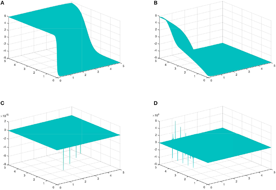
Figure 1. Physical features with suitable values of the parameters. (A) M-truncated with γ = 0.5, β = 0.9 for (27). (B) Beta with γ = 0.5 for (27). (C) M-truncated with γ = 0.5, β = 0.9 for (28). (D) Beta with γ = 0.5, β = 0.9 for (27).

FIGURE 2

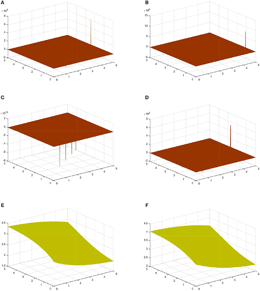
Figure 2. Physical features with suitable values of the parameters. (A) M-truncated with γ = 0.5, β = 0.9 for (29). (B) Beta with γ = 0.5 for (29). (C) M-truncated with γ = 0.5, β = 0.9 for (30). (D) Beta with γ = 0.5, β = 0.9 for (30). (E) M-truncated with γ = 0.85, β = 0.76 for (39). (F) Beta with γ = 0.85 for (39).

FIGURE 3

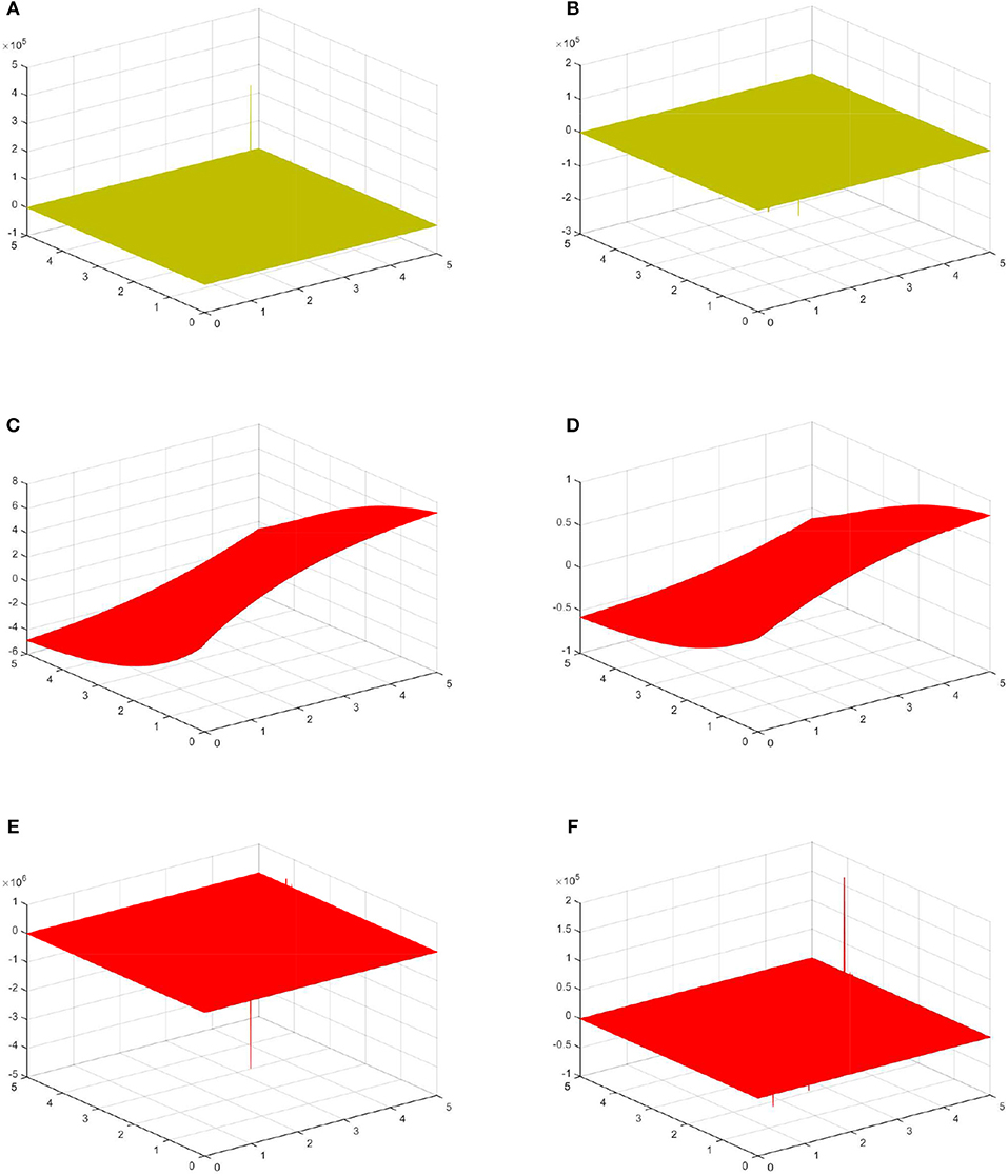
Figure 3. Physical features with suitable values of the parameters. (A) M-truncated with γ = 0.85, β = 0.76 for (40). (B) Beta with γ = 0.85, β = 0.9 for (40). (C) M-truncated with γ = 0.85, β = 0.76 for (41). (D) Beta with γ = 0.85 for (41). (E) M-truncated with γ = 0.85, β = 0.76 for (42). (F) Beta with γ = 0.85, β = 0.9 for (42).

Data Availability

All datasets generated for this study are included in the manuscript and the supplementary files.

Author Contributions

All authors listed have made a substantial, direct and intellectual contribution to the work, and approved it for publication.

Conflict of Interest Statement

The authors declare that the research was conducted in the absence of any commercial or financial relationships that could be construed as a potential conflict of interest.

The handling editor is currently organizing a Research Topic with one of the authors DB, and confirms the absence of any other collaboration.

References

1. Diethelm K. The Analysis of Fractional Differential Equations. Berlin: Springer (2010).

Google Scholar

2. Miller KS, Ross B. An Introduction to the Fractional Calculus and Fractional Differential Equations. New York, NY: Wiley (1993).

3. Podlubny I. Fractional Differential Equations. San Diego, CA: Academic Press (1999).

Google Scholar

4. Oldham KB, Spanier J. The Fractional Calculus. San Diego, CA: Academic Press (1974).

Google Scholar

5. Bas E, Ozarslan R. Real world applications of fractional models by Atangana-Baleanu fractional derivative. Chaos Solitons Fractals. (2018) 116:121–5. doi: 10.1016/j.chaos.2018.09.019

CrossRef Full Text | Google Scholar

6. El-Sayed AMA, Gaber M. The Adomian decomposition method for solving partial differential equations of fractal order in finite domains. Phys Lett A. (2006) 359:175–82. doi: 10.1016/j.physleta.2006.06.024

CrossRef Full Text | Google Scholar

7. Mirzazadeh M, Eslami M, Biswas A. Dispersive optical solitons by Kudryashov's method. Optik. (2014) 125:6874–80. doi: 10.1016/j.ijleo.2014.02.044

CrossRef Full Text | Google Scholar

8. Nazarzadeh A, Eslami M, Mirzazadeh M. Exact solutions of some nonlinear partial differential equations using functional variable method. Pramana. (2013) 81:225–36. doi: 10.1007/s12043-013-0565-9

CrossRef Full Text | Google Scholar

9. Osman MS, Korkmaz A, Rezazadeh H, Mirzazadeh M, Eslami M, Zhou Q. The unified method for conformable time fractional Schrodinger equation with perturbation terms. Chin J Phys. (2018) 56:2500–6. doi: 10.1016/j.cjph.2018.06.009

CrossRef Full Text | Google Scholar

10. Ghanbari B, Yusuf A, Inc M. Dark optical solitons and modulation instability analysis of nonlinear Schrodinger equation with higher order dispersion and cubic-quintic nonlinearity. J Coupled Syst Multiscale Dyn. (2018) 6:217–27. doi: 10.1166/jcsmd.2018.1160

CrossRef Full Text | Google Scholar

11. Qureshi S, Yusuf A, Shaikh AA, Inc M, Baleanu D. Fractional modeling of blood ethanol concentration system with real data application. Chaos (2019) 29:013143. doi: 10.1063/1.5082907

PubMed Abstract | CrossRef Full Text | Google Scholar

12. Qureshi S, Yusuf A. Modeling chickenpox disease with fractional derivatives: from caputo to atangana-baleanu. Chaos Solit Fract. (2019) 122:111–8. doi: 10.1016/j.chaos.2019.03.020

CrossRef Full Text | Google Scholar

13. Qureshi S, Yusuf A. Fractional derivatives applied to MSEIR problems: comparative study with real world data. Eur Phys J Plus. (2019) 134:171. doi: 10.1140/epjp/i2019-12661-7

CrossRef Full Text | Google Scholar

14. Younas B, Younis M, Ahmed MO, Rizvi STR. Exact optical solitons in (n + 1)-dimensions under anti-cubic law of nonlinearity. Optik. (2018) 156:479–86. doi: 10.1016/j.ijleo.2017.11.148

CrossRef Full Text | Google Scholar

15. Tariq KU, Younis M, Rizvi STR. Optical solitons in monomode fibers with higher order nonlinear Schrodinger equation. Optik. (2018) 154:360–71. doi: 10.1016/j.ijleo.2017.10.035

CrossRef Full Text | Google Scholar

16. Ashraf R, Ahmad MO, Younis M, Tariq KU, Rizvi STR. Dipole and combo solitons in DWDM systems. Optik. (2018) 158:1073–9. doi: 10.1016/j.ijleo.2017.12.201

CrossRef Full Text | Google Scholar

17. Inc M, Abdel-Gawad HI, Tantawy M, Yusuf A. On multiple soliton similariton-pair solutions, conservation laws via multiplier and stability analysis for the Whitham-Broer-Kaup equations inweakly dispersive media. Math Meth Appl Sci. (2019) 42:2455–64. doi: 10.1002/mma.5521

CrossRef Full Text

18. Nawaz B, Rizvi STR, Ali K, Younis M. Optical soliton for perturbed nonlinear fractional Schrodinger equation by extended trial function method. Opt Quant Electr. (2018) 50:204. doi: 10.1007/s11082-018-1468-2

CrossRef Full Text | Google Scholar

19. Yusuf A, Inc M, Baleau D. Optical solitons possessing beta derivative of the Chen-Lee-Liu equation in optical fibers. Front. Phys. (2019) 7:34. doi: 10.3389/fphy.2019.00034

CrossRef Full Text | Google Scholar

20. Abdel-Gawad HI, Tantawy M, Inc M, Yusuf A. On multi-fusion solitons induced by inelastic collision for quasi-periodic propagation with nonlinear refractive index and stability analysis. Mod Phys Lett B. (2018) 32:1850353. doi: 10.1142/S0217984918503530

CrossRef Full Text | Google Scholar

21. Ghanbari B, Yusuf A, Inc M, Baleanu D. The new exact solitary wave solutions and stability analysis for the (2+1)-dimensional Zakharov-Kuznetsov equation. Adv Diff Equat. (2019) 2019:49. doi: 10.1186/s13662-019-1964-0

CrossRef Full Text | Google Scholar

22. Eslami M, Neirameh A. New exact solutions for higher order nonlinear Schrodinger equation in optical fibers. Opt Quant Electr. (2018) 50:47. doi: 10.1007/s11082-017-1310-2

CrossRef Full Text | Google Scholar

23. Eslami M, Mirzazadeh M. Optical solitons with Biswas Milovic equation for power law and dual-power law nonlinearities. Nonlin Dyn. (2016) 83:731–8. doi: 10.1007/s11071-015-2361-1

CrossRef Full Text | Google Scholar

24. Eslami M, Rezazadeh H. The first integral method for Wu Zhang system with conformable time-fractional derivative. Calcolo. (2016) 53:475–85. doi: 10.1007/s10092-015-0158-8

CrossRef Full Text | Google Scholar

25. Khodadad FS, Nazari F, Eslami M, Rezazadeh H. Soliton solutions of the conformable fractional Zakharov Kuznetsov equation with dual-power law nonlinearity. Opt Quant Electr. (2017) 49:384. doi: 10.1007/s11082-017-1225-y

CrossRef Full Text | Google Scholar

26. Eslami M, Mirzazadeh M. First integral method to look for exact solutions of a variety of Boussinesq-like equations. Ocean Eng. (2014) 83:133–7. doi: 10.1016/j.oceaneng.2014.02.026

CrossRef Full Text | Google Scholar

27. Biswas A, Mirzazadeh M, Eslami M, Milovic D, Belic M. Solitons in optical metamaterials by functional variable method and first integral approach. Frequenz. (2014) 68:525–30. doi: 10.1515/freq-2014-0050

CrossRef Full Text | Google Scholar

28. Ekici M, Mirzazadeh M, Eslami M. Solitons and other solutions to Boussinesq equation with power law nonlinearity and dual dispersion. Nonlin Dyn. (2016) 84:669–76. doi: 10.1007/s11071-015-2515-1

CrossRef Full Text | Google Scholar

29. Mirzazadeh M, Eslami M, Biswas A. 1-Soliton solution of KdV6 equation. Nonlin Dyn. (2015) 80:387–96. doi: 10.1007/s11071-014-1876-1

CrossRef Full Text | Google Scholar

30. Rezazadeh H, Korkmaz A, Eslami M, Vahidi J, Asghari R. Traveling wave solution of conformable fractional generalized reaction Duffing model by generalized projective Riccati equation method. Opt Quant Electr. (2018) 50:150. doi: 10.1007/s11082-018-1416-1

CrossRef Full Text | Google Scholar

31. Zhou Q, Ekici M, Sonmezoglu A, Mirzazadeh M, Eslami M. Optical solitons with Biswas Milovic equation by extended trial equation method. Nonlin Dyn. (2016) 84:1883-900. doi: 10.1007/s11071-016-2613-8

CrossRef Full Text | Google Scholar

32. Eslami M. Trial solution technique to chiral nonlinear Schrodinger's equation in (1+ 2)-dimensions. Nonlin Dyn. (2016) 85:813–6. doi: 10.1007/s11071-016-2724-2

CrossRef Full Text | Google Scholar

33. Mirzazadeh M, Eslami M, Zerrad E, Mahmood MF, Biswas A, Belic M. Optical solitons in nonlinear directional couplers by sine cosine function method and Bernoulli's equation approach. Nonlin Dyn. (2015) 81:1933–49. doi: 10.1007/s11071-015-2117-y

CrossRef Full Text | Google Scholar

34. Neirameh A, Eslami M. An analytical method for finding exact solitary wave solutions ofthe coupled (2 1)-dimensional Painlev Burgers equation. Sci Iran. (2017) 24:715–26. doi: 10.24200/sci.2017.4056

CrossRef Full Text | Google Scholar

35. Neirameh A, Eslami M. New travelling wave solutions for plasma model of extended K-dV equation. Afrika Matematika. (2019) 30:335–44. doi: 10.1007/s13370-018-00651-2

CrossRef Full Text | Google Scholar

36. Mirzazadeh M, Eslami M, Biswas A. Soliton solutions of the generalized Klein Gordon equation by using $(\frac{G^{\prime }}{G})$ G' G-expansion method. Comput Appl Math. (2014) 33:831–9. doi: 10.1007/s40314-013-0098-3

CrossRef Full Text | Google Scholar

37. Eslami M. Solutions for Space Time Fractional (2+ 1)-Dimensional Dispersive Long Wave Equations. Iran J Sci Technol Trans A. (2017) 41:1027–32. doi: 10.1007/s40995-017-0320-z

CrossRef Full Text | Google Scholar

38. Eslami M, Rezazadeh H, Rezazadeh M, Mosavi SS. Exact solutions to the space time fractional Schrdinger Hirota equation and the space time modified KDV Zakharov Kuznetsov equation. Opt Quant Electron. (2017) 49:279. doi: 10.1007/s11082-017-1112-6

CrossRef Full Text | Google Scholar

39. Podlubny I. Fractional Differential Equations: An Introduction to Fractional Derivatives, Fractional Differential Equations, to Methods of TheirSolution and Some of Their Applications. New York, NY: Academic Press (1998). p. 198.

40. Oldham KB, Spanier J. The Fractional Calculus. New York, NY: Academic Press (1974).

Google Scholar

41. Singh J, Kumar D, Al Qurashi M, Baleanu D. A new fractional model for giving up smoking dynamics. Adv Differ Equ. (2017) 2017:88. doi: 10.1186/s13662-017-1139-9

CrossRef Full Text | Google Scholar

42. Caputo M, Mainardi F. A new dissipation model based on memory mechanism. Pure Appl. Geophys. (1971) 91:134–47. doi: 10.1007/BF00879562

CrossRef Full Text | Google Scholar

43. Bas E, Acay B, Ozarslan R. Fractional models with singular and non-singular kernels for energy efficient buildings. Chaos. (2019) 29:023110. doi: 10.1063/1.5082390

PubMed Abstract | CrossRef Full Text | Google Scholar

44. Atangana A, Baleanu D. New fractional derivatives with nonlocal and non-singular kernel. Theory Appl Heat Transfer Model Therm Sci. (2016) 20:763–9. doi: 10.2298/TSCI160111018A

CrossRef Full Text | Google Scholar

45. Atangana A, Secer A. A note on fractional order derivatives and table of fractional derivatives of some special functions. Abstr Appl Anal. (2013) 2013:279681. doi: 10.1155/2013/279681

CrossRef Full Text | Google Scholar

46. Khalil R, Al Horani M, Yousef A, Sababheh M. A new definition of fractional derivative. J Comput Appl Math. (2014) 264:65–70. doi: 10.1016/j.cam.2014.01.002

CrossRef Full Text | Google Scholar

47. Acay B, Bas E, Abdeljawad T. Non-local fractional calculus from different viewpoint generated by truncated M-derivative. J Comput Appl Math. (2019) 366:112410. doi: 10.1016/j.cam.2019.112410

CrossRef Full Text | Google Scholar

48. Sousa JVDC, de Oliveira EC. A new truncated M-fractional derivative type unifying some fractional derivative types with classical properties. Int J Anal Appl. (2018) 16:83–96.

Google Scholar

49. Scott AC. Encyclopedia of Nonlinear Science. New York, NY: Routledge, Taylor and Francis Group (2005).

Google Scholar

50. Mirzazadeh M, Ekici M, Sonmezoglu A, Eslami M, Zhou Q, Kara AH, et al. Optical solitons with complex Ginzburg-Landau equation. Nonlin Dyn. (2016) 85:1979–2016. doi: 10.1007/s11071-016-2810-5

CrossRef Full Text | Google Scholar

51. Shwetanshumala S. Temporal 1-soliton solution of the complex Ginzburg-Landau equation with power law nonlinearity. Prog Electromagn Res Lett. (2009) 96:1–7. doi: 10.2528/PIER09073108

CrossRef Full Text

52. Tian B, Gao YT. On the generalized Tanh method for the (2+1)-dimensional breaking soliton equation. Modern Phys Lett A. (1995) 10:2937–41. doi: 10.1142/S0217732395003070

CrossRef Full Text | Google Scholar

53. Inc M, Yusuf A, Isa AI, Baleanu D. Dark and singular optical solitons for the conformable space-time nonlinear Schrodinger equation with Kerr and power law nonlinearity. Optik. (2018) 162:65–75. doi: 10.1016/j.ijleo.2018.02.085

CrossRef Full Text | Google Scholar

54. Rosenau P, Hyman JM, Staley M. Multidimensional compactons. Phys Rev Lett. (2007) 98:024101. doi: 10.1103/PhysRevLett.98.024101

PubMed Abstract | CrossRef Full Text | Google Scholar

55. Camassa R, Holm DD. An integrable shallow water equation with peaked solitons. Phys Rev Lett. (1993) 71:1661–4. doi: 10.1103/PhysRevLett.71.1661

PubMed Abstract | CrossRef Full Text | Google Scholar

56. Keiser G. Optical Fiber Communications, 4th Edn. New York, NY: Tata McGraw-Hill (2008).