Numerical Study of Electron Cyclotron Drift Instability: Application to Hall Thruster

Introduction

Hall thrusters (HTs) [1–4] are ExB plasma-based devices used for Space application. In the most common coaxial version, electrons are emitted from an external cathode (working also as ion plume neutralizer), while the anode neutral propellant injector is fixed upstream at the beginning of the channel. A radial (the cylindrical reference system will be used in the rest of the paper) magnetic field lowers the electron mobility along the axial direction leading to a double effect: (1) generate an axial electric field in proximity of the exit plane that accelerates the un-magnetized propellant ions (usually noble gases) without the necessity of any extraction grid; therefore, HTs do not suffer from the limitation of the Child-Langmuir law and are characterized by a relatively high acceleration efficiency; (2) generate an azimuthal closed ExB drift v_de and increase the electron residence time inside the channel in order to guarantee an high level of ionization.

Nevertheless, the measured electron cross-field mobility results hundreds times larger [4] than its classical collisional-induced value

$\begin{array}{ll}{\mu }_{cl}=\frac{\frac{\left|q\right|}{m_e{v}_m}}{1+\frac{{\omega }_{ce}^2}{v_m^2}}.& (1)\end{array}$

Here, m_e and q are the electron mass and charge, while ν_m and ω_ce are the electron collisional and cyclotron frequencies, respectively.

Despite numerous studies on different physical mechanisms involved in HTs, the problem of electron anomalous transport across the magnetic field remains an open issue. Among the different mechanisms proposed [5–9] to explain the electron anomalous transport, the most plausible candidate is the electron ExB drift instability [10, 11] generated by the unbalanced electron Hall current. It results in azimuthal modulations of electron/ion density and azimuthal electric field whose frequency and wavelength of the order of MHz and mm, respectively, have been observed in different experiments [12]. The correlation between electron density n_e and azimuthal electric field E_θ, equivalent to a friction force density [10, 11]

$\begin{array}{ll}{f}_{ei}=q\langle n_e{E}_{\theta }\rangle & (2)\end{array}$

between the rotating electrons and almost immobile ions along the azimuthal direction, gives an extra contribution to the electron cross-field mobility (derived by electron momentum conserving equation taking into account azimuthal instabilities [10])

$\begin{array}{ll}{\mu }_{eff}={\mu }_{cl}\left[1-\frac{{\omega }_{ce}}{v_m}\frac{\langle n_e{E}_{\theta }\rangle }{n_{e0}{E}_{z0}}\right].& (3)\end{array}$

where n_e0 and E_z0 represent the azimuthally averaged electron density and accelerating axial field, respectively.

This instability has been analyzed in detail by different 1D-azimuthal Particle-in-Cell (PIC) [13, 14] models [15–20] assuming fixed axial electric and radial magnetic fields in Cartesian geometry (often used due to the high value of the external diameter to channel with ratio) and using a periodicity length along the azimuthal coordinate always smaller than the real one (Figure 1 represents the corresponding simulation domain).

FIGURE 1

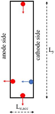
Figure 1. Sketch of the simulation domain used for 1D-azimuthal PIC simulation of HTs. L_y is the size of the azimuthal domain, while L_z,acc represent the distance traveled by electrons and ions before to be re-injected from the opposite side.

In these models steady state solutions are reached only if particle losses along the virtual axial boundaries are included. In fact, particles are still tracked along the axial direction (even if their position is not used to self-consistently calculate the axial electric field) and each electron (resp. ion) leaving the simulation domain on the anode (resp. cathode) side is replaced by a new electron (resp. ion) at the cathode (resp. anode) side loaded with an half-Maxwellian velocity distribution with the initial temperature. This particle re-injection mechanism, necessary to avoid undesirable secular effect and to mimic the axial transport, works like an extra collision: reducing the axial-replacement length L_z,acc is equivalent to increase the collisional frequency in a 1D-azimuthal model. Usually, the value chosen corresponds to the acceleration region, where both the axial electric and radial magnetic fields can be considered uniform. Probably, no replacement can be still used only if one is interested to just characterize the linear stage of the instability occurring in <1 μs. However, in order to represent the following non-linear evolution and saturation, an axial re-placement is essential.

All these studies have confirmed a significant fluctuation amplitude of ExB drift instability characterized during the linear stage by high-frequency (of the order of MHz) and discrete number of short-wavelengths (the dominant one of the order of mm) corresponding to cyclotron harmonics

$\begin{array}{ll}{\lambda }_{ExBEDI,m}=\frac{2\pi }{m}\frac{v_{de}}{{\omega }_{ce}}.& (4)\end{array}$

where m is an integer. An important feature observed is the difference in the ion and electron density fluctuations. While the electron density perturbation has lower amplitude sinusoidal character, the ion density perturbation is characterized by much larger amplitudes and contains shorter wavelengths (non-quasineutral) with λ ≤ λ_De (λ_De being the electron Debye length) producing highly-localized cnoidal structures with sharper crests and flatter troughs more.

The saturation mechanisms of the instability have been identified in the electron heating, deformation of the electron distribution function projected along the azimuthal direction and ion-wave trapping. The non-linear stage evolution of the instability instead has given controversial results: some models [17] show a transition of the mode into the regime of the ion-sound instability typical of un-magnetized plasmas, while other models [18] suggest that the magnetic field remains important in the mechanism of the instability, electron heating, and transport. This discrepancy can be attributed to the intrinsic limitation of missing the axial coordinate. In fact, in [17] a re-injection criterion is used while in [18] the particles are kept throughout the simulation as with an infinite acceleration length.

In all the models, the computed cross-field mobility has very large values (one order of magnitude larger) compared with that measured in HTs. The last point can be related to the fact that the acceleration field E_z0 is externally imposed and kept fixed, while one expects that an increase of the local mobility would yield a decrease of the local electric field, which would reduce the drift velocity and control the possible instabilities leading to the anomalous electron transport.

Recent models [20–25] have added the radial coordinate resolving the direction along the magnetic field and accounting for the sheath boundary conditions. They have shown that the full ion sound regime is not realized, but a more effective regime of discrete cyclotron resonance instabilities occur. The magnetic field remains to be a defining feature of ExB drift instability for HT operational regime. On the contrary, the scaling of wavelength, frequency and amplitude of the azimuthal field obtained within azimuthal-axial models [19, 26–30] is consistent with the ion acoustic like character of the instability

$\begin{array}{ll}{\lambda }_{IAI}\approx 2\sqrt{2}\pi {\lambda }_{De}& (5)\end{array}$

$\begin{array}{ll}\omega \approx \frac{1}{\sqrt{3}}{\omega }_{pi}& (6)\end{array}$

$\begin{array}{ll}\left|E_{\theta }\right|~\frac{T_e}{{\lambda }_{De}}& (7)\end{array}$

(ω_pi and T_e are ion plasma frequency and electron temperature, respectively).

All the azimuthal models show that results are very sensitive to the numerical parameters used. Instabilities require a very good resolution both in space/time and particle number, in order to have the modes well represented and running up to non-linear and saturation regimes. In particular, numerical noise is responsible for the destruction of electron cyclotron resonance and facilitates the transition to an ion acoustic instability. For this reason, in this work, we have preferred to develop a 1D-azimuthal model by using a high-statistical level. In the next section, the model is explained in detail and the effect of the different re-injection methods is presented. Section Reference Case and Effect of Periodicity Length is devoted to the effect of the azimuthal length of the simulation domain on the evolution of the wave spectrum. The scaling of the mobility as a function of plasma density, neutral density, magnetic field, electric field, and ion mass has been conducted in section Parametrical Study and Scaling Laws. Finally, the conclusions have been drawn in the last section Conclusions.

Description of the Model and Numerical Convergence Study

The numerical method used is based on electrostatic 1D-azimuthal Particle in Cell / Monte Carlo Collision (PIC-MCC) methodology [13, 14]. Uniform radial magnetic B₀ and axial electric field E_z0 are kept fixed during the simulation that starts loading the particles (electrons and ions) uniformly along the azimuthal and axial directions of the simulation domain (represented in Figure 1) and with a prescribed velocity distribution. Electrons and ions are both initialized with a shifted-Maxwellian distribution: electrons at a temperature T_e0 and with an azimuthal drift v_de = E_z0/B₀, ions with a temperature T_i0 and an axial drift $v_{id}=\sqrt{2q{E}_{z0}{L}_{z,acc}/M}$ (M is the ion mass) corresponding to the velocity acquired by the ions in the acceleration region. Differently from the other components, the axial component of ion velocity is not updated during the simulation and considered as frozen (approximation well-posed since ions are treated as collisionless). All the physical parameters used are summarized in Table 1.

TABLE 1

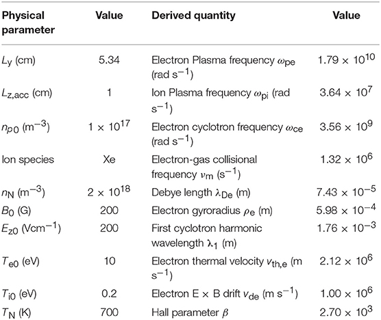
Table 1. Physical parameter used in the test case.

The cartesian approximation is adopted neglecting the effect of the presence of the centrifugal force. From now on we will use y to represent the azimuthal coordinate θ. The time-step used is Δt = 2x10⁻¹² s.

The self-consistent electric field is solved along the ExB direction with a Thomas tridiagonal algorithm modified to implement periodic boundary conditions [31]. The reference zero potential value is put at the boundaries.

Electron-neutral collisions (elastic scattering, electronic excitation, and ionization) are included. In order to keep the averaged plasma density equal to the initial condition selected, we assume that during the ionization event, only the energy loss and scattering is taken into account, while then new electron-ion pair is not produced.

In the present model, we consider the particle re-injection across the axial boundaries. Differently from [17] the re-injected particles are not randomly distributed along the azimuthal direction but they keep their azimuthal positions. They just change their velocity components, exactly like in an inelastic collisional event. This choice is dictated by the fact that, with a random y-location re-injection, a large charge imbalance is artificially created amplified by the fact that the model is one-dimensional. A certain space-charge density (difference between electrons reaching the anode side and ions crossing the cathode one) is created along the ExB direction that generates an artificially high azimuthal electric field. In the 2D-radial-azimuthal extension of the model [25], the random re-injection has much less impact due to the fact that the charge injected is also distributed along the radial dimension. Furthermore, we have verified that results obtained with random azimuthal re-injection are sensitive to the couple of parameters (L_y, L_z,acc) chosen, as already observed in [17]. For small L_y (≤1 cm) or large L_z,acc (>2 cm), the reference potential or the low rate of particles re-injected help to keep the azimuthal electric field low.

Figure 2 shows the temporal evolution of the averaged (over the particle population) electron (blue curve) and ion (red curve) energy when re-injected particles are loaded with random y-position (Figure 2A) and when they keep their own azimuthal position had just before the re-injection (Figure 2B) using L_y = 2.67 cm and L_z,acc = 1 cm. In the first case, both electron and ion energy increase reaching already after 3 μs unphysical values due to the large azimuthal electric field induced by the random re-injection.

FIGURE 2

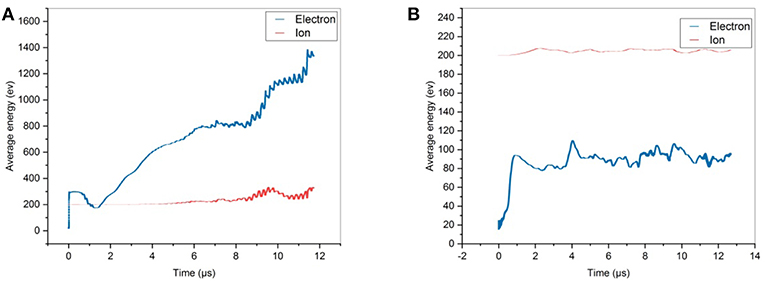
Figure 2. Averaged electron and ion energy with particle re-injection method across the axial boundaries (A) with random azimuthal positions and (B) preserving azimuthal positions. Results correspond to a case using physical parameters reported in Table 1 (but using an azimuthal simulation domain length of L_y = 2.67 cm) with number of particles per cell N_ppc = 500 and mesh nodes N_g = 1,000 (corresponding to a cell size Δy = 0.36λ_De).

Due to the high sensitivity shown by previous models on the numerical parameters used, we have studied the numerical convergence. The global quantities taken as monitoring observables are the electron cross-field mobility and electron density fluctuation level. In case of 1D-azimuthal PIC representation, the mobility can be simply extracted from the averaged axial velocity

$\begin{array}{ll}{\mu }_{PIC}=\frac{{\displaystyle {\sum }_{ip=1}^{N_p}}{v}_{ip,ez}}{N_p{E}_{z0}}& (8)\end{array}$

where v_ip,ez is the axial component of the electron velocity and N_p is the total number of particles used in the simulation. The physical condition used are that summarized in Table 1.

Figure 3A shows the electron cross-field mobility and Figure 3B shows the amplitude of fluctuations in electron density computed as a function of number of particles per cell N_ppc (from 20 to 1,000) for four different numbers of mesh nodes, N_g = 250, 500, 1,000, and 2,000, corresponding to four different values of cell size to Debye length ratio $\frac{\Delta y}{{\lambda }_D}=$ 1.44, 0.72, 0.36, and 0.18. Results correspond to a time larger than 10 μs and the mobility and fluctuation amplitude reported were also time averaged over the last 2 μs. In addition, the time series of electron averaged energy for different N_ppc with N_g = 1,000 and for different N_g with N_ppc = 500 have also been reported in Figures 3C,D, respectively. For N_ppc >500 all the cases give results close to the averaged value of μ_PIC = 3.4 m²V⁻¹s⁻¹ within a deviation <5% and fluctuations in the electron density around 22% of the equilibrium density. The electron heating growth rate does not change if using N_ppc larger than 500 and N_g larger than 1,000. Therefore, for the rest of the work, we have fixed the numerical parameters at N_ppc = 500 and $\frac{\Delta y}{{\lambda }_D}=$ 0.36.

FIGURE 3

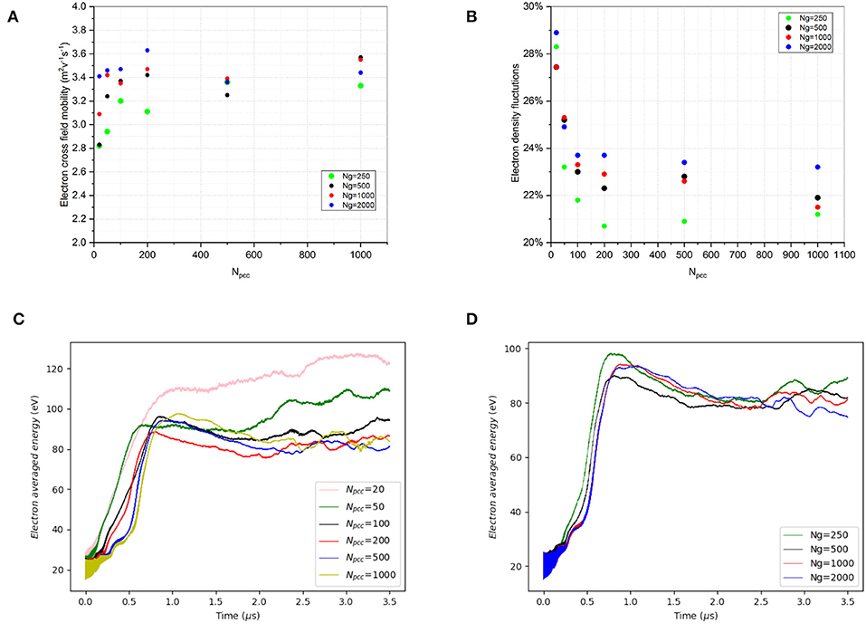
Figure 3. (A) Computed mobility using Equation (8) and (B) amplitude of fluctuations in electron density as a function of the number of particles per cell N_ppc for four different cell size $\frac{\Delta y}{{\lambda }_{De}}=$1.44 (number of mesh nodes N_g = 250), 0.72 (N_g = 500), 0.36 (N_g = 1,000) and 0.18 (N_g = 2,000). Electron averaged energy evolution for different N_ppc using N_g = 1,000 (C) and for different N_g using N_ppc = 500 (D). All the cases correspond to physical parameters reported in Table 1 using azimuthal length of L_y = 2.67 cm.

Reference Case and Effect of Periodicity Length

In this section we present results obtained using physical data reported in Table 1. It is considered as reference case for the physical parametrical scan study reported in the next section Parametrical study and scaling laws.

Figure 4 shows an overview of the simulation run. The history of the global averaged electron / ion energy and electrostatic potential energy density $u_E=\frac{1}{2}{\epsilon }_0{E}_y^2$ are displayed over a total time of 5 μs. In the graph one can identify four stages: (1) the linear growth, a very fast process terminating already after the first microsecond; (2) the first non-linear stage ending at t = 3.5 μs and during which the electron energy appears to saturate; this phase corresponds to a redistribution of the spectral energy toward lower harmonics (see Figure 6B) and to the ion heating; (3) the second non-linear phase when the electron and ion energy rise again; (4) the final quasi-steady state reached after t = 4.5 μs.

FIGURE 4

Figure 4. Electron (red curve), ion (blue curve) averaged energy and electrostatic potential energy density (black curve) in the simulation up to t = 5 μs. Results refer to the reference case using physical parameters reported in Table 1.

Figure 5 show the azimuthal profiles of Figure 5A electron (red curve) and ion (blue curve) density and Figure 5B oscillating electric field at t = 12 μs, after the saturation, in the non-linear regime. Profiles confirm large amplitude coherent mode driven at the fundamental cyclotron harmonic λ₁ = 1.72 mm [Equation (4) with m = 1 gives λ_{ExB−EDI, m = 1} = 1.76 mm] with a marked cnoidal character for the ion density modulation, effect of the localized ion trapping (see end of this section), together with the presence of a large scale envelope.

FIGURE 5

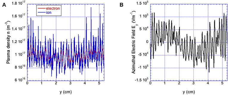
Figure 5. Azimuthal profiles of (A) electron (red curve) ion (blue curve) density and (B) azimuthal electric field at t = 12 μs. Results refer to the reference case using physical parameters reported in Table 1.

Figure 6A shows the time evolution of the azimuthal profile of E_y and Figure 6B shows the time evolution of the corresponding power spectral density (PSD) into wavenumber k_y = 2π/λ components. The instability starts during the linear stage (for t<2 μs) with the growth of the most instable cyclotron harmonics (seven different harmonics are easily distinguishable from the spectrum) whose dominant one has the following characteristics: wavelength k = 3,650 m⁻¹ [corresponding to the first cyclotron harmonic m = 1 of Equation (4)], frequency ω = 4.8 MHz and phase velocity v_ϕ = 8 km/s in the ExB drift direction. However, the values found are also in good agreement with Equation (5), the theoretical estimation of an ion acoustic character found in Lafleur et al. [11] using the wavenumber with the maximum growth. Using an electron temperature of T_e = 60 eV (computed in the non-linear phase, see Figure 7C) Equation (5) gives k_IAI = 3,890 m⁻¹, while Equation (6) gives ω = 3.2 MHz. In the next section Parametrical study and scaling laws, a dedicated study is conducted to distinguish the true character of instability.

FIGURE 6

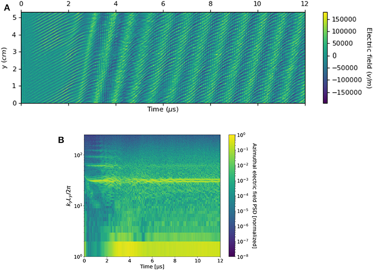
Figure 6. Temporal evolution of (A) the azimuthal profile of the oscillating electric field E_y and of (B) the corresponding distribution of power into wavenumber components S_Ey(k_y).

FIGURE 7

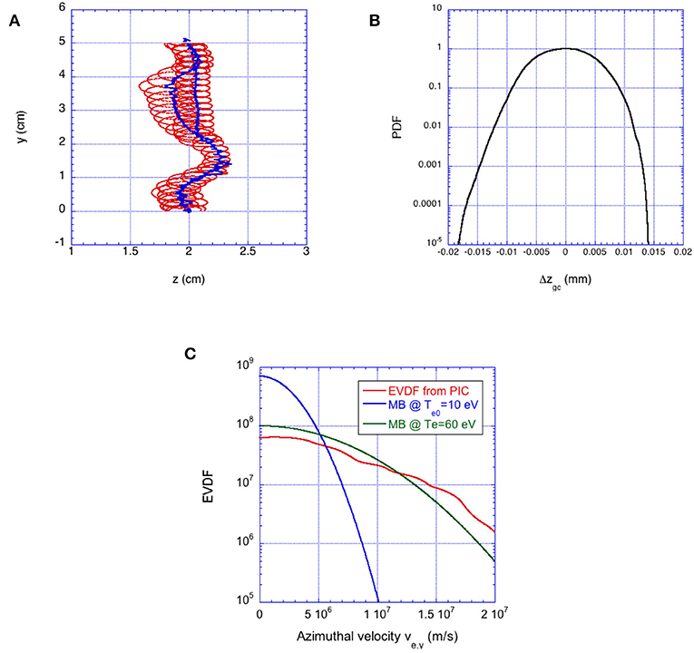
Figure 7. (A) Trajectory of a sampled electron (red curve) and its guiding center (blue curve) during the non-linear phase (total sampling time corresponding to 0.1 μs). (B) Probability distribution function (PDF normalized to the maximum) of the electron guiding centers jump size Δz_gc. (C) Azimuthal velocity distribution function of electrons at t = 12 μs (red curve). The Maxwell distribution functions given as reference have the initial temperature set in the model T_e0 = 10 eV (blue curve) and the equivalent temperature from best fitting the computed distribution (green curve).

For t>2 μs, the highest cyclotronic harmonics are strongly attenuated. The resonance character of the ExB EDI based on the linear treatment and Maxwellian behavior of electron distribution function, disappears by a resonance broadening mechanism [32]. Only the first harmonic remains detectable making the electrons still keeping their magnetization even if much weaker: electrons trajectories are deformed by the azimuthal wave of electric field and slightly elongated in the direction parallel to E_z0 (see Figure 7A). A simple criterion for resonance destruction [18] (corresponding to impose an electron displacement Δz_e larger than the half-wavelength over one cyclotron period):

$\begin{array}{ll}{\left(\frac{{\omega }_{pe}}{{\omega }_{ce}}\right)}^2\frac{|E_k{|}^2}{8\pi }>\frac{{n_{p}T}_e}{k{\rho }_e}& (9)\end{array}$

highlights the dependence on the electron temperature for the different k-modes: the highest wavenumbers are faster damped requiring a smaller electron temperature threshold. Electrons can also move to the right, but in average they diffuse toward the left as evident from the asymmetry of the probability distribution function of the electron guiding centers jump size Δz_{e, gc} reported in Figure 7B.

Figure 7C shows the origin of the resonance broadening, i.e., the deformation of the electron velocity distribution function: its projection along the azimuthal direction at the end of the simulation (red curve) is compared with the initial Maxwellian distribution at T_e0 = 10 eV (blue curve) and with its Maxwellian best fitting (green curve). The latter shows that electrons heat up to a level of T_e = 60 eV due to their continuous trapping and de-trapping induced by the bouncing into the potential well-created by wave field. The electron heating create a strong phase-space mixing of the electron distribution function leading to a marked low-energy range depletion and electron velocity distribution function (EVDF) flattening.

Furthermore, a very low k-number component (much lower than the fundamental cyclotron mode k₁) appears corresponding to wavelengths comparable to the entire simulation domain size (k_yL_y/2π = 1 in Figure 6B). Already previous 1D-azimuthal and 2D-radial-azimuthal models [18, 23, 25] have shown non-linear development of large-scale modes, comparable to the entire azimuthal size of the simulation domain. For this reason, we have investigated the effect of the periodicity length imposed to the model studying different cases with L_y = 0.67, 1.34, 2.68, and 5.36 cm (the latter corresponding to one quarter the real length of the SPT100 HT), using the physical parameters of Table 1 and numerical parameters fixed at the end of section Description of the model and numerical convergence study. The wavenumber spectrum of the oscillating field E_y in the non-linear stage (t = 12 μs) is reported in Figure 8 for the two cases L_y = 0.67 cm (red curve) and L_y = 5.36 cm (blue curve). As evident, both reveals the presence of the same dominant cyclotron harmonic k₁ = 3,650 m⁻¹, but using a larger simulation domain, new low-k modes appear whose amplitude are comparable to that of the dominant cyclotron harmonic. We have verified that the large wavelength mode is not associated with the particle re-injection method by observing that it is still present in the case without re-injection (already at t = 2 μs before the electron energy grows beyond an acceptable value).

FIGURE 8

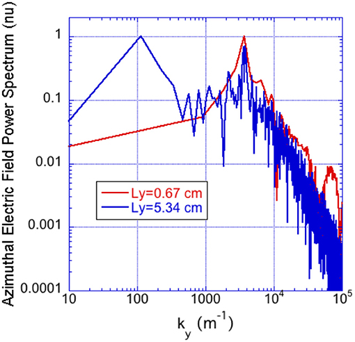
Figure 8. Amplitudes (normalized to the maximum) of E_y spectral components k_y using two different azimuthal domain size. Results correspond to input data reported in Table 1 and using the following numerical parameters N_ppc = 500 and $\frac{\Delta y}{{\lambda }_D}=$ 0.36.

Finally, the instability is observed to stabilize when the amplitude is large enough to trap a significant portion of ions: the confirmation comes from the ion heating and rotation since the free energy dissipates by giving the ion distribution a long tail, rather than driving exponentially growing azimuthal electric field. Figure 9A shows the ion velocity distribution function (IVDF) projected along the azimuthal direction (red curve) and (Figure 9B) the corresponding ion phase space at t = 12 μs. In Figure 9A are also reported for comparison the initial Maxwellian distribution at T_i = 0.2 eV (blue curve) and the Maxwellian best fitting the computed IVDF (green curve). The latter gives a final temperature of T_i = 10 eV, fifty times larger than the initial one. Moreover, the ion rotation occurs with the presence of different ion beams. In particular, two populations are distinguishable, one dominant rotating with a fluid velocity of about 13 km/s and another minor population rotating with 20 km/s. Figure 9B clearly shows the vortex formation typical characteristic of trapping in the azimuthal wave.

FIGURE 9

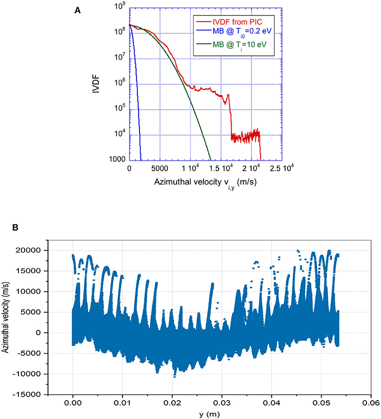
Figure 9. (A) Distribution function of ions and (B) corresponding ion phase space at t = 12 μs (red curve). The Maxwell distribution functions given as reference have the initial temperature set in the model T_i0 = 0.2 eV (blue curve) and the equivalent temperature from best fitting the computed distribution (green curve).

Parametrical Study and Scaling Laws

Since operating parameters (Table 1) are very effective on the ExB EDI and as a consequence, on the global electron cross-field transport, we are interesting to conduct a study of the behavior of the electron cross-field mobility [calculated following Equation (8)] as a function of the most important input data used: neutral density, plasma density, magnetic field, accelerating electric field, and ion mass. In addition, the total cross-field mobility derived by electron momentum conserving equation taking into account azimuthal instabilities, Equation (3), is also used for comparison. The azimuthal correlation between the electron density and azimuthal electric field is computed in the PIC model through a double integral formula by using a time-averaged (over an interval T = 2 μs) value

$\begin{array}{ll}\langle n_e{E}_y\rangle ={\displaystyle {\int }_0^{Ly}}{\displaystyle {\int }_0^T}\frac{dy}{Ly}\frac{dt}{T}{n}_e(y,t)E_y(y,t)& (10)\end{array}$

discretized using the Simpson's 1/3 rule [33].

Figure 10A shows the gas density dependence keeping the other physical parameters fixed to the values reported in Table 1. This study allows knowing the effect of collisions on the mobility since the contribution of instability does not depend on the electron-neutral collisional frequency. At very low gas density, the contribution to the electron cross-field mobility predominantly comes from the instability: its initial value is mostly determined by the second term on the right-hand side of Equation (3). However, we must remember that the particle re-injection technique adopted (see section Description of the model and numerical convergence study) corresponds to an artificial collision always present even in the case of very low gas density. As the gas density increases the collisional contribution becomes stronger (mixed regime) and the cross-field mobility increases reaching its maximum for n_N = 8 × 10²⁰ m⁻³. For much larger gas density the regime is collision-dominated [the first term on the right-hand side of Equation (3) is dominant]: the mobility change behavior decreasing as the gas density increases following the classical collisional dependence Equation (1) (for ν_m ≫ ω_ce) ${\mu }_{\perp }\propto \frac{1}{n_N}$.

FIGURE 10

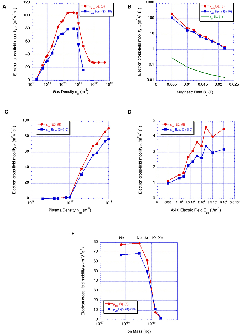
Figure 10. Calculated steady state cross-field mobility as a function of (A) xenon gas density, (B) magnetic field, (C) plasma density, (D) axial electric field and (E) ion mass, using data reported in Table 1.

Figure 10B shows the electron cross-field mobility as a function of the magnetic field imposed. Both estimations follows the classical behavior Equation (1) ${\mu }_{\perp }\propto \frac{1}{B^2}$ (green curve), but the effective collisional frequency ν_{m, eff} results 50 times larger than the real value reported in Table 1. This proof that in HT regime, the electron ExB drift instability does not induce full turbulence Bohm-like behavior ${\mu }_{\perp ,Bohm}\propto \frac{1}{B}$.

Figure 10C shows the electron cross-field mobility as a function of the plasma density studying the pure effect of the instability on the electron transport (the gas density is kept fixed to n_N = 2 × 10¹⁸ m⁻³). In agreement with values found by previous PIC simulations [16, 17], the mobility always increases with the plasma density starting from the pure collisional value assumed at very low plasma density (no instability) given by Equation (1) ${\mu }_{\perp }=1.8x10^{-2}{m}^2{V}^{-1}{s}^{-1}$.

In Figure 10D the behavior of the electron mobility as a function of the applied axial electric field is reported. A larger E_z0 gives larger ExB drift and therefore stronger electron cyclotron instability. As a consequence the mobility shows a continuous growth in the range analyzed.

Figure 10E reports the effect of the ion mass, where the most relevant noble gases (He, Ne, Ar, Kr, and Xe) have been used. The different cases all use the same cross section in order to avoid possible contamination on the mobility due to the different cross sections, and measure in this way the pure ion mass effect. As evident, heavier ions lead to a strong reduction (larger than 10 times) of the electron cross-field mobility. The behavior is in agreement with the kinetic theoretical treatment of [11] that have shown as the onset conditions for instability are reduced and the unstable region is broader for lighter ions.

Finally, the parametrical study has been used to understand the character of the instability after the non-linear evolution. The case study using physical parameters reported in Table 1 leads to very similar wavelengths, whatever is the character of the instability, λ_{ExB EDI} = 1.76 mm and λ_IAI = 1.62 mm. It is not useful to identify the nature of the instability at saturation occurred. However, by observing Equations (4) and (5), one can see that the ExB EDI wavelength scales with the axial electric field and radial magnetic field, while the ion-acoustic wave scales with the electron density and temperature. In Figure 11A we have reported the k-spectrum of the electron density at t = 10 μs for four different electron density, n_p0 = 2 × 10¹⁶, 4 × 10¹⁶, 5 × 10¹⁶, and 8 × 10¹⁶ m⁻³, while Figure 11B shows the dominant wavelength computed in the non-linear phase as a function of magnetic field B₀ (blue circles) and accelerating electric field E_z0 (red circles) using as electron density n_p0 = 1 × 10¹⁷ m⁻³. As evident, the dominant wavelength does not depend on the electron density (i.e., on the Debye length since the electron temperature computed does not change with the density) and perfectly scales according to the electron cyclotron drift instability Equation (4). However, it has to be pointed out that, the missing axial coordinate can play an important role in hindering the ion acoustic like transition since azimuthal-axial models [19, 26–30] have always shown a scaling according to ion acoustic like character of the instability Equation (5).

FIGURE 11

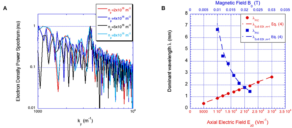
Figure 11. (A) Amplitudes (normalized to the maximum) of n_e spectral components k_y using four different electron density. (B) Dominant wave detected in the non-linear phase as a function of magnetic field B₀ (blue circles using E_z0 = 200 Vcm-1) and accelerating electric field E_z0 (red circles using B₀ = 200 G). Results correspond to input data reported in Table 1 and using the following numerical parameters N_ppc = 500 and $\frac{\Delta y}{{\lambda }_D}=$ 0.36.

Conclusions

In this work, we have presented a numerical study, based on 1D Particle-in-Cell methodology, of the electron ExB drift instability in Hall thruster. It gives correlated fluctuations in electron density and electric field leading to enhanced electron cross-field mobility. The local representation is simplified since it neglects any effects of axial gradients, radial contributions, and assumes a constant axial electric field. Nevertheless, the description allows having a high statistical level, condition necessary to reduce the effect of numerical heating on the linear and non-linear evolution and on saturation of the instability.

Results show that fluctuation spectra remain quantized (electron magnetization signature) predominantly retaining the fundamental cyclotron mode. In addition, using larger azimuthal simulation domains (forcing the periodicity length toward a realistic value), the development of long wavelength envelope comparable to the entire azimuthal extension, appears.

An accurate parametrical study has also been conducted to find the behavior of electron cross-field mobility as a function of the most important operative quantities: gas and plasma density, magnetic field, axial electric field, and ion mass. The electron cross-field transport shows a strong dependence on the plasma density and ion mass. The computed dominant wavelength scales according to the ExB EDI and no transition toward ion acoustic like instability is observed.

Data Availability Statement

The datasets generated for this study are available on request to the corresponding author.

Author Contributions

FT developed the numerical method and led the manuscript preparation. ZA contributed to the code development and to the article preparation. FT, ZA, and MS contributed to the analysis and discussion of the results.

Funding

This work was supported by the Apulia Space Project (grant PON03PE_00067_6).

Conflict of Interest

The authors declare that the research was conducted in the absence of any commercial or financial relationships that could be construed as a potential conflict of interest.

Acknowledgments

The authors would like to thank Pierpaolo Minelli and Guillaume Bogopolsky for their help with the code implementation and result graphics.

References

1. Zhurin VV, Kaufman HR, Robinson RS Physics of closed drift thrusters. Plasma Sour Sci Technol. (1999) 8:R1. doi: 10.1088/0963-0252/8/1/021

CrossRef Full Text | Google Scholar

2. Morozov AI, Savelyev VV. Fundamentals of stationary plasma Thruster theory. In: Kadomtsev BB, Shafranov VD, editors. Reviews of Plasma Physics. Reviews of Plasma Physics, Vol 21. Boston, MA: Springer (2000). p. 203–391. doi: 10.1007/978-1-4615-4309-1_2

CrossRef Full Text | Google Scholar

3. Goebel DM, Katz I. Fundamentals of Electric Propulsion: Hall and Ion Thrusters. Hoboken, NJ: John Wiley & Sons (2008). doi: 10.1002/9780470436448

CrossRef Full Text | Google Scholar

4. Boeuf JP. Tutorial: physics and modeling of Hall thrusters. J Appl Phys. (2017) 121:011101. doi: 10.1063/1.4972269

CrossRef Full Text | Google Scholar

5. Morozov AI, Savelyev VV. Theory of the near-wall Conductivity. Plasma Phys Rep. (2001) 27:570–5. doi: 10.1134/1.1385435

CrossRef Full Text | Google Scholar

6. Janes GS, Lowder RS. Anomalous electron diffusion and ion acceleration in a low-density plasma. Phys Fluids. (1966) 9:1115–23. doi: 10.1063/1.1761810

CrossRef Full Text | Google Scholar

7. Scharfe MK, Thomas CA, Scharfe DB, Gascon N, Cappelli MA, Fernandez E. Shear-based model for electron transport in hybrid Hall thruster simulations. IEEE Trans Plasma Sci. (2008) 36:2058–68. doi: 10.1109/TPS.2008.2004364

CrossRef Full Text | Google Scholar

8. Cappelli MA, Young CV, Cha A, Fernandez E. A zero-equation turbulence model for two-dimensional hybrid Hall thruster simulations. Phys Plasmas. (2015) 22:114505. doi: 10.1063/1.4935891

CrossRef Full Text | Google Scholar

9. Jorns B. Predictive, data-driven model for the anomalous electron collision frequency in a Hall effect thruster. Plasma Sour Sci Technol. (2018) 27:104007. doi: 10.1088/1361-6595/aae472

CrossRef Full Text

10. Lafleur T, Baalrud SD, Chabert P. Theory for the anomalous electron transport in Hall effect thrusters. II. Kinetic model. Phys Plasmas. (2016) 23:053503. doi: 10.1063/1.4948496

CrossRef Full Text | Google Scholar

11. Lafleur T, Baalrud SD, Chabert P. Characteristics and transport effects of the electron drift instability in Hall-effect thrusters. Plasma Sour Sci Technol. (2017) 26:024008. doi: 10.1088/1361-6595/aa56e2

CrossRef Full Text | Google Scholar

12. Tsikata S, Honoré C, Lemoine N, Grésillon DM. Three-dimensional structure of electron density fluctuations in the Hall thruster plasma: ExB mode. Phys Plasmas. (2010) 17:112110. doi: 10.1063/1.3499350

CrossRef Full Text | Google Scholar

13. Hockney RW, Eastwood JW. Computer Simulation Using Particles. New York, NY: IOP Publishing Ltd (1989).

Google Scholar

14. Birdsall CK, Langdon AB. Plasma Physics Via Computer Simulation. New York, NY: Taylor and Francis (2005).

Google Scholar

15. Ducrocq A, Adam JC, Héron A, Laval G. High-frequency electron drift instability in the cross-field configuration of Hall thrusters. Phys Plasmas. (2006) 13:102111. doi: 10.1063/1.2359718

CrossRef Full Text | Google Scholar

16. Boeuf JP. Rotating structures in low temperature magnetized plasmas—insight from particle simulations. Front Phys. (2014) 2:74. doi: 10.3389/fphy.2014.00074

CrossRef Full Text | Google Scholar

17. Lafleur T, Baalrud SD, Chabert P. Theory for the anomalous electron transport in Hall effect thrusters. I. Insights from particle-in-cell simulations. Phys Plasmas. (2016) 23:053502. doi: 10.1063/1.4948495

CrossRef Full Text | Google Scholar

18. Janhunen S, Smolyakov A, Chapurin O, Sydorenko D, Kaganovich I, Raitses Y. Nonlinear structures and anomalous transport in partially magnetized ExB plasmas. Phys Plasmas. (2018) 25:011608. doi: 10.1063/1.5001206

CrossRef Full Text | Google Scholar

19. Katz I, Chaplin H, Lopez Ortega A. Particle-in-cell simulations of Hall thruster acceleration and near plume regions. Phys. Plasmas. (2018) 25:123504. doi: 10.1063/1.5054009

CrossRef Full Text | Google Scholar

20. Hara K. An overview of discharge plasma modeling for Hall effect thrusters. Plasma Sour Sci Technol. (2019) 28:044001. doi: 10.1088/1361-6595/ab0f70

CrossRef Full Text | Google Scholar

21. Héron A, Adam JC Anomalous conductivity in Hall thrusters: Effects of the non-linear coupling of the electron-cyclotron drift instability with secondary electron emission of the walls. Phys Plasmas. (2013) 20:082313. doi: 10.1063/1.4818796

CrossRef Full Text | Google Scholar

22. Croes V, Lafleur T, Bonaventura Z, Bourdon A, Chabert P 2D particle-in-cell simulations of the electron drift instability and associated anomalous electron transport in Hall-effect thrusters. Plasma Sour Sci Technol. (2017) 26:034001. doi: 10.1088/1361-6595/aa550f

CrossRef Full Text | Google Scholar

23. Janhunen S, Smolyakov A, Sydorenko D, Jimenez M, Kaganovich I, Raitses Y. Evolution of the electron cyclotron drift instability in two-dimensions. Phys Plasmas. (2018) 25:082308. doi: 10.1063/1.5033896

CrossRef Full Text | Google Scholar

24. Tavant A, Croes V, Lucken R, Lafleur T, Bourdon A, Chabert P. The effects of secondary electron emission on plasma sheath characteristics and electron transport in an ExB discharge via kinetic simulations. Plasma Sour Sci Technol. (2018) 27:124001. doi: 10.1088/1361-6595/aaeccd

CrossRef Full Text | Google Scholar

25. Taccogna F, Minelli P, Asadi Z, Bogopolsky G. Numerical studies of the ExB electron drift instability in Hall thrusters. Plasma Sour Sci Technol. (2019) 28:064002. doi: 10.1088/1361-6595/ab08af

CrossRef Full Text | Google Scholar

26. Adam JC, Héron A, Laval G. Study of stationary plasma thrusters using two-dimensional fully kinetic simulations. Phys Plasmas. (2004) 11:295. doi: 10.1063/1.1632904

CrossRef Full Text | Google Scholar

27. Coche P, Garrigues L A two-dimensional (azimuthal-axial) particle-in-cell model of a Hall thruster. Phys Plasmas. (2014) 21:023503. doi: 10.1063/1.4864625

CrossRef Full Text | Google Scholar

28. Lafleur T, Chabert P The role of instability-enhanced friction on ‘anomalous' electron and ion transport in Hall-effect thrusters. Plasma Sour Sci Technol. (2018) 27:015003. doi: 10.1088/1361-6595/aa9efe

CrossRef Full Text | Google Scholar

29. Lafleur T, Martorelli R, Chabert P, Bourdon A. Anomalous electron transport in Hall-effect thrusters: comparison between quasi- linear kinetic theory and particle-in-cell simulations. Phys Plasmas. (2018) 25:061202. doi: 10.1063/1.5017626

CrossRef Full Text | Google Scholar

30. Boeuf JP, Garrigues L. ExB electron drift instability in hall thrusters: particle-in-cell simulations vs. theory. Phys Plasmas. (2018) 25:061204. doi: 10.1063/1.5017033

CrossRef Full Text | Google Scholar

31. Napolitano M. A FORTRAN subroutine for the solution of periodic block-tridiagonal systems. Commun Appl Numer Meth. (1985) 1:11–15. doi: 10.1002/cnm.1630010104

CrossRef Full Text | Google Scholar

32. Muschietti L, Lembège B. Microturbulence in the electron cyclotron frequency range at perpendicular supercritical shocks. J Geophys Res. (2013) 118:2267–85. doi: 10.1002/jgra.50224

CrossRef Full Text | Google Scholar

33. Sadiku MNO. Numerical Techniques in Electromagnetics. 2nd ed. Boca Raton, FL: CRC Press (2001).

Google Scholar