Measuring Absolute Cell Volume Using Quantitative-Phase Digital Holographic Microscopy and a Low-Cost, Open-Source, and 3D-Printed Flow Chamber

Introduction

Animal cell membranes are highly permeable to water. Movements of water across the membranes are in large part dictated by osmotic pressure gradients. Consequently, even at constant extracellular osmolarity, volume constancy of any mammalian cell is permanently challenged by its own activity including, for example, movements of different ionic species across the cell membrane or transport of osmotically active substances involved in cell metabolism all of which induce osmotic water movements [1, 2]. On the other hand, a variety of vital cell functions, including enzyme activity, gene expression mechanisms, second messenger cascades, and hormone releases are all extremely dependent on a homeostatic intracellular ionic environment [3, 4]. Therefore, cell volume is one of the critical cell parameters and is closely regulated. Accordingly, cells have developed numerous efficient volume regulatory mechanisms involving multiple ion transport processes including channels, cotransporters, and exchangers which operate to maintain a constant ionic balance and hydrostatic pressure gradient. To do so, osmotically active solutes (mainly inorganic ions such as Na⁺, K⁺, Cl⁻, or organic osmolytes) are gained or lost to regulate the cell volume [5].

Currently, reliable and non-invasive measurements of the absolute cell volume V_c are difficult to achieve [6]. Although current and common flow cytometry techniques offer tremendous high-throughput capability and can be seen as the gold standard, they are dedicated to the measurement of V_c using large samples of isolated cells in suspension [7]. Nevertheless, studying volume homeostasis and its regulatory mechanisms requires the ability to be able to measure V_c within the environmental conditions in which cells grow, migrate, and communicate with one another. In this case, there is no methodological consensus to be able to achieve such V_c measurements. Among the few suitable techniques, dye exclusion microscopy, either based on absorption [8] or fluorescence [9], use the equivalent displacement of stained liquid created by a cell to measure its thickness, but this requires extracellular labels. This thickness measurement is used in conjunction with the projected cell surface (in this instance, measured in the corresponding microscopy image) to calculate V_c.

Alternatively, quantitative-phase imaging (QPI) consists of an ensemble of microscopy techniques offering the possibility of performing label-free, non-invasive, high-resolution, and real-time imaging of transparent microscopic specimens such as living cells in culture [10, 11]. QPI measures the minute phase shift, namely the quantitative-phase signal (QPS), that transparent specimens induce on the diffracted wave-front, as long as the observed sample is a weakly-scattering object, i.e., differing from the surrounding medium only by a slight difference of refractive index [12–17]. The QPS, proportional to the optical path length (OPL), thus depends on both the intracellular refractive index (IRI) and the cell thickness. According to the seminal work of Barer [18], this IRI dependency has allowed the development of QPI as an efficient technique to quantitatively monitor cellular dry mass dynamics, particularly in connection with the cell growth cycle [19–22]. Different QPI approaches based on interferometric principles have also succeeded to detect cell membrane fluctuations at the nanometric scale, especially with respect to red blood cells [23–25].

Despite these fruitful applications in simple cases, the information on the intrinsic mix of cell content and morphology, the QPS, and its variations, remain generally difficult to interpret in cell biology [26]. Measuring the IRI and the cell thickness separately represents thus the key scientific step leading to the calculation of various quantitative cellular biophysical parameters, including V_c [27, 28], the osmotic membrane water permeability [29], the refractive index of transmembrane water and solute flux [29], allowing the study of specific physiological and pathophysiological cellular processes [30–33]. Specifically, V_c is calculated from both the cell thickness and the projected cell surface, as in the case of dye exclusion microscopy.

Optical diffraction tomography makes it possible to obtain, also from the QPS, both the refractive index distribution and the morphology of living cells in 3D [34, 35]. However, this unique 3D capability comes at the price of complex imaging setups and relies heavily on the approximations used in the algorithms of the reconstruction process which requires considerable expertise to be used.

However, less complicated experimental procedures have been developed to extract both the IRI and the corresponding cell thickness from the QPS [26, 36–42], which greatly promotes their application. Conceptually, there are two main classes of such procedures. The first involves the extraction of the IRI by cell thickness evaluation either by shape approximation using geometrical models, direct measurement with complementary imaging modalities or physical confinement in the axial direction using microstructures with a priori known geometry. While the shape approximation and the physical confinement are more suited for suspended rather than adherent cells, the direct measurement with a complementary imaging modality is usually conducted separately, making the observation of dynamic biological processes cumbersome. The second group of procedures solves the IRI and the cell thickness coupling problem by achieving two different QPS measurements resulting in a system of independent linear equations with two unknowns having a unique solution. Among these techniques is the two-liquid decoupling approach which is particularly attractive for adherent cells as it does not require any cell morphology assumptions, nor axial constraining, generally resulting in better physiological environmental conditions than in those in the first class of procedures. Used in conjunction with quantitative-phase digital holographic microscopy (QP-DHM), it provides accurate measurements of the average refractive index ${\overline{n}}_c$ and the mean thickness ${\overline{h}}_c$ of a cellular body [26]. However, this technique has several drawbacks related to its washout process arising from the requirement to sequentially perfuse two different equi-osmolar physiological solutions with different, but a priori, known refractive indices.

Recent developments in affordable and precise 3D printers, as well as the availability of computer aided-design (CAD) software through additive manufacturing, offer a great opportunity to create custom-made and innovative devices that meet the needs of a specific application. For researchers, 3D printing is a versatile and inexpensive technique that allows rapid prototyping, and appreciable improvements of previous versions and variations of a design [43]. Within the context of live-cell imaging, 3D printing is therefore ideal to create microscope accessories tailored to fit the precise needs of QP-DHM, and with QPI in a more general manner.

To our knowledge, the authors have created the first, low-cost, open-source, and 3D-printed flow chamber with tailor-made flow field characteristics that produces an efficient washout process. Within the framework of the two-liquid decoupling approach, such a washout process is characterized by an early stage during which the QPS is temporally unstable, followed by a period of QPS stabilization corresponding to a state where the refractive index of the second solution is distributed in a spatially uniform way, throughout the flow chamber. From a fluid mechanics point of view, the use of a steady-state and a fully-developed laminar flow (which reduces lateral mixing) may be beneficial in this situation.

The design and scientific particularities of this 3D-printed flow chamber will be presented in this paper. First, the mechanical design of the do-it-yourself flow chamber is presented. Second, the optimization of the geometry of the flow chamber to obtain such a flow of fluid (resulting from numerical simulations), will be explained. In addition, the presence of a steady-state and fully-developed laminar flow has been confirmed experimentally for the geometry of the flow chamber. In such a situation, the washout time required to alternate between the two liquids has been extensively experimentally characterized. The rapidity at which the QPS stabilizes (an indication of the homogeneity of the refractive index of the perfusion medium) has been assessed. As a validation to demonstrate how this proposed 3D-printed flow chamber works, it has been used to perform decoupling experiments during the resting state of three common cell types in culture, namely primary neurons, HEK293T, and NIH3T3 cells. Specifically, both ${\overline{n}}_c$ and ${\overline{h}}_c,$ as well as their corresponding V_c, have been systematically calculated for each cell type. Furthermore, the cell viability rate inside the flow chamber has been compared to a control condition to determine its compatibility with live cell imaging. Finally, the changes of these biophysical parameters have been quantitatively evaluated during hypo-osmotic and hyper-osmotic challenges.

Theory and Principles

The cell-phase signal of each (x, y)-pixel of a quantitative-phase image of QP-DHM can be expressed as:

$\begin{array}{ll}\begin{array}{l}{\varphi }_c\left(x,y\right)=\frac{2\pi }{{\lambda }_0}\left({\displaystyle {\int }_0^{h_c\left(x,y\right)}}{n}_c\left(x,y,z\right)dz+n_m\left(H-h_c\left(x,y\right)\right)\right)\\ \end{array}& (1)\end{array}$

$\begin{array}{ll}\begin{array}{l}{\varphi }_c\left(x,y\right)=\frac{2\pi }{{\lambda }_0}\left(\left({\overline{n}}_c\left(x,y\right)-n_m\right)h_c\left(x,y\right)+n_{m}H\right)\\ \end{array}& (2)\end{array}$

where λ₀ is the free-space wavelength of the light source, z is the axial coordinate, h_c(x, y) is the cell thickness corresponding to the OPL of each pixel, n_c(x, y, z) is the 3D distribution of the IRI, ${\overline{n}}_c(x,y)=\frac{1}{h_c(x,y)}{\int }_0^{h_c(x,y)}{n}_c(x,y,z)dz$ is the mean value of the IRI along h_c(x, y) (otherwise known as the integral IRI), n_m is the refractive index of the perfusion medium, and H is the thickness of the flow chamber. Similarly, the phase signal corresponding to the background of a quantitative-phase image can be formulated as:

$\begin{array}{ll}\begin{array}{l}{\varphi }_{bkgd}=\frac{2\pi }{{\lambda }_0}{n}_{m}H\\ \end{array}& (3)\end{array}$

Monitoring and subsequently reusing this background value are important because this compensates for mechanical and thermal instabilities of the setup during the experiment. In addition, by considering limited background regions around the cell under study, effective variations in the chamber height are not an issue [44]. By subtracting Equation (3) from Equation (2), the QPS of each (x, y)-pixel [12] can be expressed as:

$\begin{array}{ll}\begin{array}{l}\Delta {\varphi }_c\left(x,y\right)={\varphi }_c\left(x,y\right)-{\varphi }_{bkgd}=\frac{2\pi }{{\lambda }_0}\left({\overline{n}}_c\left(x,y\right)-n_m\right)h_c\left(x,y\right)\\ \end{array}& (4)\end{array}$

Although temporal dependency is not explicitly indicated in Equation (4), it remains valid for each quantitative-phase image of a time-lapse. The dual dependence expressed by Equation (4) (known as the refractive index-thickness coupling problem [45]) results in a counterintuitive and challenging interpretation of the QPS.

In order to obtain these two contributions independently, a two-liquid decoupling procedure [26] was performed. In this method, two iso-osmotic and iso-tonic perfusion media having two different but a priori known refractive indices (namely n_m1 and n_m2) were sequentially perfused. The extracellular refractive index of the perfusion medium varied from n_m1 to n_m2 with a transient period during which the QPS is not defined, followed by a stabilization period. Meanwhile, a time-lapse of quantitative-phase images was recorded. This two-liquid decoupling approach created a system of two equations with two unknowns that can be solved as:

$\begin{array}{ll}\begin{array}{l}{\overline{n}}_c\left(x,y\right)=\frac{\Delta {\varphi }_{c_2}\left(x,y\right)n_{m_1}-\Delta {\varphi }_{c_1}\left(x,y\right)n_{m_2}}{\Delta {\varphi }_{c_2}\left(x,y\right)-\Delta {\varphi }_{c_1}\left(x,y\right)}\\ \end{array}& (5)\end{array}$

$\begin{array}{ll}\begin{array}{l}{h}_c\left(x,y\right)=\frac{{\lambda }_0}{2\pi }\frac{\Delta {\varphi }_{c_2}\left(x,y\right)-\Delta {\varphi }_{c_1}\left(x,y\right)}{n_{m_1}-n_{m_2}}\\ \end{array}& (6)\end{array}$

where the subscripts 1 and 2 refer to two different QPS stabilized states corresponding to the two different perfusion media [26]. From there, the calculation of ${\overline{n}}_c$ and ${\overline{h}}_c$ can be performed by averaging, for each state i = 1, 2, Δϕ_ci(x, y) over all the segmented pixels contained in a single-cell body, namely ${\Delta \overline{\varphi }}_{c_i}=\Delta {\varphi }_{c_i}(\overline{x},\overline{y})$. Therefore, we obtain:

$\begin{array}{ll}{\overline{n}}_c=\frac{\Delta {\overline{\varphi }}_{c_2}{n}_{m_1}-{\Delta \overline{\varphi }}_{c_1}{n}_{m_2}}{\Delta {\overline{\varphi }}_{c_2}-{\Delta \overline{\varphi }}_{c_1}}& (7)\end{array}$

$\begin{array}{ll}{\overline{h}}_c=\frac{{\lambda }_0}{2\pi }\frac{\Delta {\overline{\varphi }}_{c_2}-{\Delta \overline{\varphi }}_{c_1}}{n_{m_1}-n_{m_2}}& (8)\end{array}$

From the automated segmentation, the projected surface of the cell, S_c, is obtained which makes it possible to calculate the absolute cell volume [29], V_c, as follows:

$\begin{array}{ll}\begin{array}{c}{V}_c={\int }_{S_c}{h}_c\left(x,y\right)ds={\overline{h}}_c{S}_c\cong {\overline{h}}_c{A}_p{N}_c\\ \end{array}& (9)\end{array}$

where A_p is the area of a magnified pixel, and N_c is the number of pixels corresponding to the cell body. However, the following working assumptions must be fulfilled to obtain accurate results. It is assumed that ${\overline{n}}_c$ and ${\overline{h}}_c$ do not exhibit significant variations during the delay caused by the washout process. This notably requires the use of two equi-osmolar perfusion media to avoid any osmotic challenges. Furthermore, in order to minimize the effect of cell changes that take place over time and affecting either ${\overline{n}}_c$ or ${\overline{h}}_c$ (or both), the washout process allowing a return of the extracellular refractive indices over the entire imaging slit, toward the known values of either n_m1 or n_m2, must be as short as possible.

Materials and Methods

Fabrication of the Flow Chamber

The mechanical design of the flow chamber was drawn with SolidWorks (2016, Dassault Systèmes). The flow chamber was 3D-printed with high-strength PETG plastic (Guideline, Taulman3D) using the Ultimaker 2 Extended+ printer. The base and the lid were printed with a 0.4 mm nozzle (Micro Swiss) with light infill. Both the base and the lid each have four circular holes meant for inserting the rare-earth magnets (5862K961, McMaster-Carr). These magnets are glued with fast-adhesive glue (5551T72, McMaster-Carr). The parafilm gasket contained in the base was cut with scissors from a sheet of parafilm (M, BEMIS). The sample holder was printed with a 0.25 mm nozzle (Micro Swiss) with 100 and 30% infill overlap. The 30% infill overlap of the central element generally prevents the internal leaks; however, it must be treated with acetone to ensure complete waterproofness considering the pressure level while the fluid is flowing [46]. Only the top (the roughest surface) of the sample holder shall be exposed to the acetone (270725, Sigma-Aldrich) vapors for the advised 15 min. Following this treatment, a clean 18 mm coverslip is pressed in the groove made for this purpose, resulting in its sealing and fixing. Pressure was applied and held on the coverslip for about 1 min, with the first 10 s being decisive. On each side of the central element, stainless steel microtubes (304F10125X006SL, MicroGroup) are partially inserted and glued with fast adhesive. Cutting the tubes is a delicate process since an inappropriate technique results in it collapsing. A sharp blade (LB, OLFA) is used to roll the microtube while applying some pressure. After several back and forth cycles, the microtubes can be cut without altering their cavity. A detailed step-by-step protocol for the fabrication of the flow chamber can be found in Appendix A.

Mounting the Flow Chamber

The chamber is intended to reduce the handling time and ensure the well-being of the studied cells in keeping with the reality of cellular imaging. First, the parafilm gasket is applied to the base. Then, a small amount of perfusion liquid is injected with a connected syringe in the upside-down sample holder which has a fixed-top window. The 18 mm coverslip containing the cell culture (the bottom coverglass), is next placed upright directly on the bottom mount and wetted with a drop of temperate medium. Then, the filled central element is rotated back and positioned on the base. The chamber is then closed by pressure from only the lid and the magnets. Finally, any air bubbles are quickly purged by gently injecting medium via the syringe fixed to the sample holder.

Computational Fluid Dynamics

Simulations were made with the computational fluid dynamics (CFD) module COMSOL Multiphysics (5.3a, COMSOL) and steady-state solutions were sought. A top-view cross-section was used to define the geometry for the simulation and assuming a 2D representation to be a satisfactory approximation. To ensure closer resemblance with the experimental setup, microtubes were included in the geometry, using their inner diameter as the entrance size. To input a laminar flow at the inlet of the flow chamber, the entrance length was calculated for each flow rate with the expression for the Reynolds number in a circular pipe, resulting in values from 1 to 2 mm. Laminar flow rates were varied from 0.2 to 5.1 mL/min at the inlet. A no-slip boundary condition was used for the edges as well as a no-pressure condition for the outlet of the flow chamber. For all the simulations, the fluid flows from right to left.

Micro-particle Image Velocimetry

The experimental flow inside the imaging slit was monitored with a micro-particle image velocimetry (μPIV) setup composed of a machine vision camera (Grasshopper3, FLIR) and a variable magnification zoom lens system (MVL-7000, NAVITAR). The camera was equipped with a monochrome 2.3-megapixel Sony IMX174 CMOS sensor with a pixel size of 5.86 μm and a maximum acquisition rate of 163 fps. The zoom was a macro lens featuring a variable focal length from 18 to 108 mm. The maximum magnification is ~1.1X at its minimum working distance of 130 mm. A volume of 200 μL was taken from a 1% w/v stock solution of polystyrene microspheres with a 104 μm average diameter (PPB-1000-5, Spherotech). Then, the microspheres were suspended in 10 mL of a 1X PBS solution containing BSA at 1 mg/mL. The solution of suspended microspheres was infused with a perfusion pump (PPS-1100, Scientifica) at equivalent continuous flow rates ranging between 0.2 and 5.1 mL/min. In total, approximately three videos per flow rate, each lasting 3 s, were recorded for all four sample holders. The TrackMate plug-in of ImageJ [47] was used to follow the trajectory of the beads in the μPIV data to obtain the experimental streamlines inside the imaging slit.

Cell Culture

Primary rat neurons were obtained from dissected brain hippocampus from neonatal rats (P0-P1), as described previously [44, 48], then plated on 18-mm borosilicate coverglass coated poly-D-lysine (GG-18-1.5, Neuvitro) and cultured for 2 weeks in Neurobasal media supplemented with B27 (LS21103049, Gibco™) to obtain mature neurons forming effective networks. Two cell lines, NIH3T3 embryonic mouse fibroblast cells (ATCC^® CRL-1658™) and human fetal HEK293T cells (ATCC^® CRL-11268™) were also used in this study. Briefly, NIH3T3 and HEK293T cells were seeded 12–24 h before imaging on 18-mm coverglass coated with matrigel (C354277, Corning™) at a density of 25,000 cells or 50,000 cells per well, respectively. Both cell lines were kept in high-glucose DMEM (10-017-CV, Corning™) supplemented with 10% bovine calf serum (97068-085, VWR) or 5% of premium grade fetal bovine serum (10158-358, VWR), respectively.

Neurons Viability Assay

A total of 10 cell cultures of rat primary neurons were prepared in two experimental groups. The five cultures of the control group were kept in a petri dish (08-772B, Fisher Scientific) and immersed in mannitol-based physiological solution without perfusion for 30 min at room temperature. The five cell cultures of the test group were placed in the flow chamber and were perfused at 2 mL/min with the same physiological solution at room temperature for 30 min. All coverslips were then stained for 3 min with a 0.04% Trypan Blue solution (MT25900CI, Fisher Scientific). Fourteen images at a 20X-magnification randomly positioned along the central line of the imaging slit, and two at a 4X-magnification centered in the imaging slit have been recorded per coverslip with a transmitted light microscope (EVOS FL, Invitrogen). Negatively- and positively-stained cells on each image were identified and manually counted with ImageJ (v1.52p, NIH) to assess the number of living and dead cells. Overall cell viability rates were calculated on the randomly positioned 20X-magnification images as they are representative of the whole cell culture, whereas the 4X-magnification images were meant to quantify cell viability in a position-dependent manner since the edges of the imaging slit are visible. In this case, images were separated into four segments parallel to the length of the imaging slit, and the living and dead cells were then separately counted in each segment.

Quantitative-Phase Digital Holographic Microscopy

A digital holographic microscope (T-1003, Lyncée Tec) based on a Mach-Zehnder interferometer was used. Within the microscope, the beam produced by a 666-nm laser diode is separated into two, forming an object wave and a reference wave. The object wave, scattered by the sample, interferes with the reference wave, producing an off-axis hologram recorded by a digital camera. The microscope objective magnification is 20X with a free working distance of 590 μm, and a NA of 0.70 (HC PL APO, Leica). The camera is equipped with a monochrome 2.3-megapixel Sony IMX174 CMOS sensor with a pixel size of 5.86 μm and capable of recording at 164 fps (acA1920-155um, Basler). The digital holograms were integrated over a period of ~100 μs and acquired at a frequency of 4 Hz. The integration time was adjusted carefully at the beginning of each imaging session to avoid any saturation in the holograms. The off-axis geometry (meaning that holograms are recorded with the object and reference waves having a small angle between their directions of propagation) allows the reconstruction of quantitative-phase images from a single recorded hologram [49]. The reconstruction of the quantitative-phase image from the hologram is numerically computed using proprietary software (Koala, Lyncée Tec) and the resulting field-of-view is 215 μm by 215 μm. The reconstruction algorithm consists of a simulation of the illumination of the recorded hologram by a digital reference wave [50]. This is followed by a numerical correction of the wave-front aberration induced by the optical components, the objective, and the off-axis geometry of the microscope using a reference-conjugated hologram [51]. As for background flattening, it has been performed by means of polynomials [52].

Two-Liquid Decoupling Approach

The two-liquid decoupling approach requires sequentially perfusing two distinct physiological solutions with the same osmolarity and different, but a priori, known refractive indices. Concretely, a small amount of NaCl (25 mM) of an iso-osmotic and isotonic medium with an osmolarity appropriate for the cell under study (i.e., 220 mOsm/kg for neurons or 340 mOsm/kg for HEK293T and NIH3T3 cells) was replaced by either 50 mM of mannitol or 50 mM of Nycodenz to obtain the two different perfusion media [26]. In practice, the refractive index and osmolarity of every physiological solution has been measured with an Abbe refractometer (Abbemat MW, Anton Paar) at 666 nm and a freezing-point osmometer (Micro-Sample model 3320, Advanced Instruments), respectively, prior to the QP-DHM session. The refractive index of the mannitol-based perfusion medium is ~1.3335, whereas for the Nycodenz-based physiological solution, it is 1.3380. Finally, consecutive perfusion of these physiological solutions, using a perfusion gravity system linked to an 8-port manual distribution valve [44], was performed either successively for three times, or before and after the cells were submitted to an osmotic challenge. For all the physiological solutions, the flow rate of the perfusion was set to 2 mL/min.

Osmotic Challenges

Three different cell types, primary hippocampal neurons, NIH3T3 cells, and HEK293T cells mounted in at least four different sample holders, were submitted to hypo-osmotic or hyper-osmotic challenges. In these experiments, the primary neurons were perfused with HEPES-buffered physiological solution with an osmolarity similar to Neurobasal + B27^® medium containing (in mM) 75 NaCl, 5.4 KCl, 1.8 CaCl₂, 0.8 MgCl₂, 0.9 NaH₂PO₄, 10 HEPES, 5 dextrose (D-glucose), 50 mannitol, or Nycodenz (pH 7.4; 225-230 mOsm). The other cell cultures (HEK293T and NIH3T3) were maintained in DMEM which has a higher osmolarity (330 mOsm), and thus were perfused with an appropriate iso-osmotic solution (in mM) 135 NaCl, 3 KCl, 5 dextrose, 10 HEPES, 3 CaCl₂, and 1.8 MgCl₂, 50 mannitol or Nycodenz (pH 7.4; 330–335 mOsm). The hypo-osmotic media were prepared by removing 25 mM of NaCl from the iso-osmotic solutions, and the hyper-osmotic media by adding 25 mM of NaCl to the iso-osmotic solutions, resulting in refractive index alterations of −0.0003 and 0.0003, respectively, from their iso-osmotic counterpart. All cells were perfused with the adequate mannitol iso-osmotic medium and the QP-DHM recording started when the QPS was stable, typically after 2 min. Usually, the baseline was recorded for ~1 min, and then replaced by the Nycodenz iso-osmotic solution required for decoupling the resting state of the cells for ~30 s. The cells were then submitted to the osmotic challenge by either perfusing for ~5 min with either the hypo-osmotic or the hyper-osmotic solution containing Nycodenz. Finally, after the osmotic challenge was completed, a second decoupling sequence was performed by changing the medium for the mannitol-based solution but having the same osmolarity as that used for the challenge, for ~1 min.

Post-processing of Quantitative-Phase Images

Rectifications are commonly applied during the numerical reconstruction of the holograms to correct phase aberrations and image distortions. However, some irregularities may nevertheless persist in the quantitative-phase images. The reference-conjugated hologram and polynomials (both determined at the beginning of the experiment) gradually degrade and lose some of their effectiveness over time. Therefore, a spline smoothing method was used to iteratively determine an illumination function that when subtracted from the quantitative-phase image, effectively offsets the background fluctuations. This correction was individually applied to each quantitative-phase image in a time series as shown in reference [44]. Thereafter, a global threshold-based segmentation strategy, implementing a minimum cross-entropy algorithm, was used to classify each pixel of the quantitative-phase image as either belonging to the background or to the foreground. In addition, an intensity-based method was used to distinguish between individual objects in the foreground that are touching one another and therefore not properly delineated as two entities by the segmentation alone. Finally, the segmented cells were numerically labeled throughout the time-lapse of quantitative-phase images to perform a cell-by-cell analysis.

Results and Discussion

As previously mentioned, an effective and accurate two-liquid decoupling approach is required to obtain a rapid and homogeneous return of the extracellular refractive index toward the known values of either n_m1 or n_m2 over the entire imaging slit of the flow chamber. Correspondingly, it is well-known in fluid mechanics that a flow system in which the pipe diameter changes abruptly from one size to another gives rise to what is referred to as vena contracta. The loss coefficient for a sudden size variation is a function of the geometry, with a sharp-edged change having more losses. Accordingly, the flow is said to separate from the sharp corner. The separated flow location is then the host of a swirl that traps the liquid and creates a counter-current flow, or an eddy. The size of such an eddy is flow rate dependent; in a faster flow, it spans a larger zone. In the context of the two-liquid decoupling approach (where two different physiological solutions are sequentially perfused), these dead volumes and unstirred layers are detrimental to obtaining a fast-homogeneous return of the extracellular refractive index toward either n_m1 or n_m2. Most available perfusion chambers have abrupt size expansions, e.g., a square-edged entrance and exit. A concrete example is the junctions between the microtubes for the perfusion and the imaging slit. These locations give rise to important losses causing separated flows containing eddies even at very low flow rates as confirmed by the CFD simulation shown in Figure 1. This simulation corresponds to a flow rate of 2 mL/min at the entrance of a rectangular imaging slit with a square-edged entrance and exit of same size as the one developed and described hereafter. Thus, a rectangular imaging slit with a square-edged entrance and exit does not allow for a fast and homogeneous washout. However, from a fluid mechanics point of view, obtaining a steady-state and fully-developed laminar flow is expected to be beneficial. Therefore, the geometry of the flow chamber has been optimized to provide such a flow field.

FIGURE 1

Figure 1. Separated flow and eddies. Flow simulation of a 2 mL/min flow rate through a rectangular imaging slit without diffusers. Streamlines are shown in black and are overlaid on the velocity field with values indicated by the color bar. The formation of a vena contracta and eddies are made evident with the separation of the flow. The flow direction is specified with the black arrow.

Mechanical Design

The exploded view of the proposed flow chamber is shown in Figure 2A. The flow chamber was 3D-printed with a plastic filament intended for medical and clinical applications since the raw material itself is biocompatible. The raw material is listed with the Food and Drug Administration and has complied with specific biocompatibility tests, namely ISO 10993, including cell cytotoxicity [43]. The sample holder contains the channel for the flow and is encapsulated by two 18-mm coverslips. The top coverglass acts as an observation window while the bottom coverslip mounts the cell culture. The parafilm gasket is placed underneath the bottom coverglass to ensure waterproofness. Stainless steel microtubes with 0.4-mm internal diameters and 0.8-mm outer diameters, are partially inserted up to the entrance of the channel in the central element to convey the perfusion medium. The base plate holds the sample holder. The entire chamber is closed using the lid and four rare-earth magnets. For sizing purposes, a mounted flow chamber (top) and a sample holder (bottom) are shown in Figure 2B.

FIGURE 2

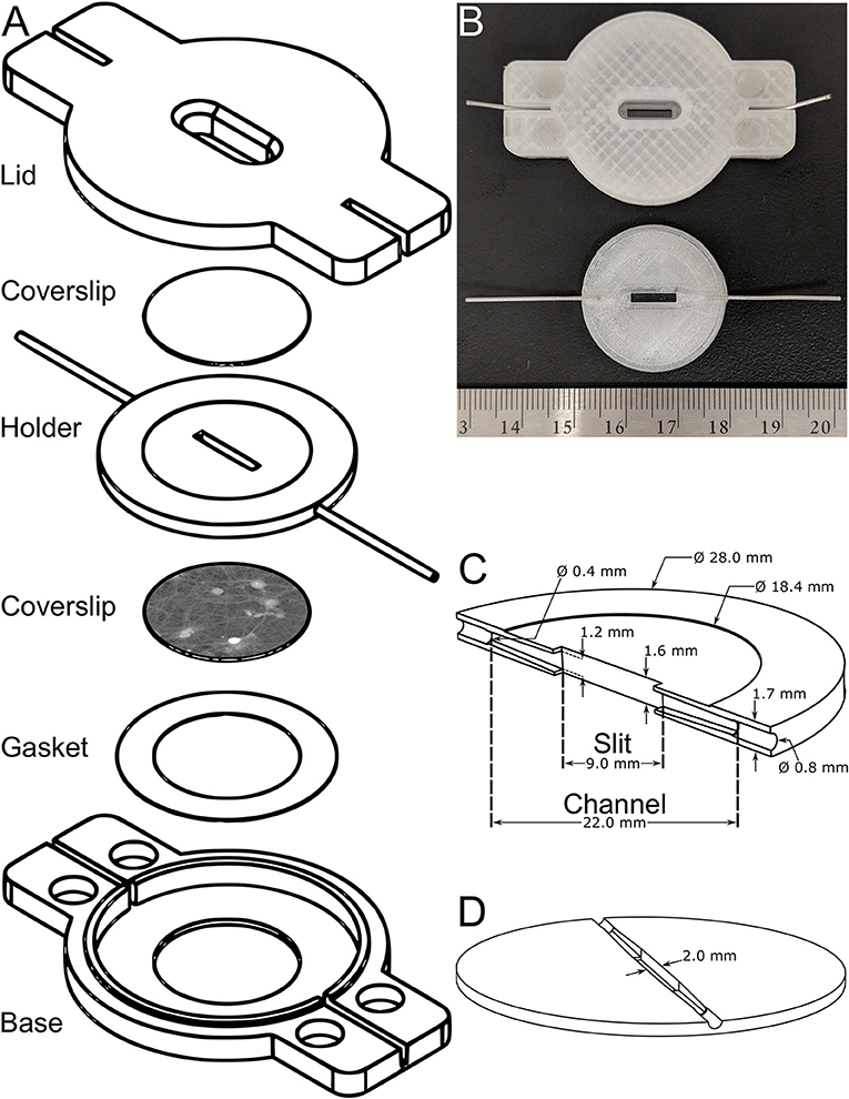
Figure 2. Mechanical design. (A) An exploded CAD-model view representing the flow chamber and detailing its constituents. (B) Photograph showing the assembled flow chamber (top) and a sample holder (bottom) as well as a ruler, for sizing purposes. (C,D) CAD models of the sample holder showing, respectively, a vertical and horizontal cross-section of the channel highlighting the diffusers where the outlet of the stainless steel microtubes will be attached to the imaging slit.

The central element, as shown in Figures 2C,D and being, respectively, a vertical and horizontal cross-section of the channel, is the key component of the flow chamber and is described in more detail in this paragraph. The channel changes smoothly from a circular cross-section of 0.4 mm in diameter (at the outlet of the stainless steel microtubes), to a rectangular cross-section 1.2-mm high and 2.0-mm wide at the level of the imaging slit using pyramidal diffusers. The opening and closing angles of these pyramidal diffusers, highlighted in Figures 2C,D, have been optimized and this aspect will be discussed in Section Steady-State and Fully-Developed Laminar Flow. The 9.0-mm long imaging slit has an area of 18.0 mm² and an internal volume of 28.8 μl. The internal volume has been voluntarily minimized to enable fast washouts. Concretely, the area of the imaging slit is ~400 times that of a typical field of view for a microscope objective having a 20x-magnification. The thickness of the sample holder cannot be further reduced because the microtubes are inserted into it. Based on a daily usage in the laboratory, the lifetime of the central element is ~3 months after which leaks may occur or a degradation of the fluidic performances may be experienced. While the lid and base outlast the lifetime of the sample holder, the gasket is designed for single use. The fabrication cost of the entire flow chamber is 12 USD, of which 0.86 USD is for the plastic itself. Printing all flow chamber parts takes ~4 h. Gluing the tubes to the sample holder and the magnets to the mounts takes 15 min. The acetone treatment takes ~30 min to complete. It is advised to wait at least 2 h after the treatment to test its water tightness. The entire process takes ~7 h, 6 of which are spent waiting. The design files of the do-it-yourself flow chamber will be shared with the scientific community through an open-source model for rapid dissemination and maximum impact. The technical drawings will be available on the web page of the authors' research group upon publication.

Steady-State and Fully-Developed Laminar Flow

A simple way to reduce the losses mentioned above is to round off the entrance and exit regions of the imaging slit which connects it to the channels. A geometry such as this, shaped to decelerate the fluid, is called a diffuser. There is an optimum angle for which the loss coefficient is minimum, which is usually around 10°. The relatively small value of this angle for minimal losses results in a long diffuser and is an indication of the fact that it is difficult to efficiently decelerate a fluid [53]. Thus, 6.5-mm long pyramidal diffusers with a total opening and closing angle of 11.45° have been added at the ends of the imaging slit as shown in Figures 2C,D. Such an angle, close to the optimal one, was chosen to have both minimal losses and an imaging slit of a size compatible with the resolution of the 3D printer. To evaluate the proposed design, CFD simulations have been computed for 16 flow rate values ranging from 0.2 to 5.1 mL/min. As an indication, the results shown in Figures 3A–C, are zoomed in on the imaging slit and the fluid flows from right to left. For synthesis purposes, only 3 of the 16 flow rates are illustrated. The field of streamlines (the black solid lines) for 1.0, 2.0, and 2.8 mL/min, superimposed on their respective velocity distributions and color coded, are shown in Figures 3A–C (top). The simulations show that fluid flows in constant-velocity parallel layers along a path parallel to the wall of the imaging slit. Adjacent layers exhibit slightly different speeds according to a velocity gradient perpendicular to the streamlines. This behavior is typical of a steady-state and fully-developed laminar flow. However, at a relatively high flow rate of 2.8 mL/min, there is a small region at the entrance where separated flow appears. For the specific application presented here, it has been noted that the Reynolds number is not a sufficiently sensitive metric to predict the presence of vortices and backward flows. As an example, at a flow rate of 5.1 mL/min, the flow chamber is completely filled with eddies, has revealed by the streamlines. But, the maximum corresponding Reynolds number is 12, well below the threshold value of 2100 from which the flow supposedly stops to be laminar, and this by a factor of ~200 (data not shown). Therefore, it is inappropriate to optimize the geometry and the sizing of the flow chamber based on this measure.

FIGURE 3

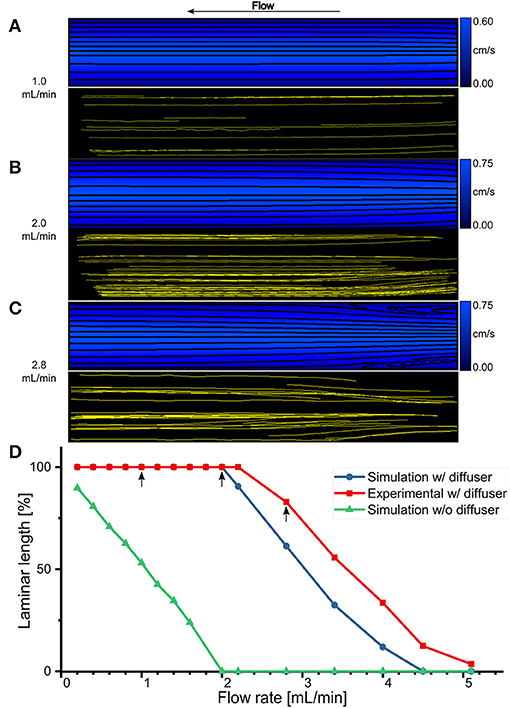
Figure 3. Steady-state and fully-developed laminar flow. (A–C) Comparison of CFD flow simulation (top) and experimental μPIV (bottom) for the imaging slit of the flow chamber with pyramidal diffusers at three different flow rates: 1.0, 2.0, and 2.8 mL/min, respectively. (D) Laminar length for an imaging slit without diffuser (green line, triangles) were obtained solely with simulations. Laminar length within the imaging slit with diffusers as a function of flow rate obtained with CFD simulations (blue line, circles) and experimental μPIV (red line, squares). Arrow indicates the flow rates shown in (A–C).

To experimentally confirm the validity of the design, μPIV experiments have been conducted using the same 16 values of flow rates as for the CFD simulations as shown in Figures 3A–C (bottom). Again, only the same three flow rates are represented. Each yellow solid line corresponds to the trajectory of a single particle inside the imaging slit flow field, therefore providing an experimental way to obtain the streamlines inside the actual flow chamber. The experimentally retrieved streamlines correspond reasonably well with those resulting from the numerical simulations. For the flow rates of 1.0 and 2.0 mL/min, the streamlines are relatively straight and parallel while for a high flow rate of 2.8 mL/min the two areas of separated flow at the entrance are observed. This stresses that the actual flow of fluid inside the imaging slit is steady-state, fully-developed, and laminar.

Since the regions of separated flow contain an eddy that traps the liquid and creates a counter-current flow, they are detrimental to obtaining a washout process characterized by a rapid stabilization of the refractive index values around n_m1 or n_m2. To quantify the extent of this phenomenon, the reattachment length L_r (defined as the distance from the entrance of the imaging slit at which the flow resumes in the positive flow direction all over the cross-section) has been measured. In order to obtain a metric that represents the laminar length L_l expressed as a percentage of the total length L_t of the imaging slit, and therefore free from separated flow regions, L_l is defined as follows: L_l = 100(L_t − L_r)/L_t. For the design having pyramidal diffusers, L_l has been measured on both the simulated (blue line, circles) and experimental data (red line, squares), and for all the studied flow rates, as shown in Figure 3D. An arrow demonstrates the three flow rates shown in Figures 3A–C. The analysis shows that the imaging slit is entirely usable, L_l = 100%, for flows up to 2 mL/min after which L_l decreases monotonically. For comparison purposes, an L_l based on CFD simulations for a rectangular imaging slit with a square-edged entrance and exit, having the same size than the proposed design comprising pyramidal diffusers, is plotted in Figure 3D. In this case, L_l is already 90% at 0.2 mL/min, and it decreases, monotonically as a function of the flow rate. It is important to note that the rectangular design contains separated flows throughout its length, L_l = 0%, at the typical flow rate for cellular imaging of 2 mL/min. At this flow rate, the proposed design comprising pyramidal diffusers is still entirely laminar.

Neurons Viability

Another important aspect of the flow chamber design is its compatibility with live cell imaging. A cell viability assay has been performed on neurons; this cell type is known to be very sensitive to environmental conditions. As shown in Figure 4A, the percentage of living neurons in the control group is 84.74 ± 2.26% while the viability in the test group is 81.71 ± 4.91%. Both viability rates are close, but the slight trend is likely to result from the additional manipulation of assembling the chamber i.e., risking a brief exposure to the air when the cells are momentarily removed from their physiological solution and again when closing the chamber. Nevertheless, this extra step is required with all perfusion chambers whether homemade or commercial in nature. However, this slight decrease in viability rate does not preclude imaging healthy cell cultures. Since neurons are more sensitive to environmental conditions than most other cell types, higher viability rates are expected for HEK293T and NIH3T3 cells. Furthermore, cells lying in the different segments of the imaging slit, as seen on Figure 4B, exhibit similar viability rates, namely 80.74 ± 7.28%, 83.68 ± 5.37%, 85.59 ± 4.17%, and 81.97 ± 7.74%, from segment one through four, respectively. Therefore, there is no significant variation in cell viability between the distinct regions of the imaging slit. Cells close to the edges of the imaging slit are not preferentially damaged nor do they obtain any benefit with respect to their viability.

FIGURE 4

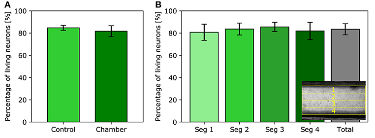
Figure 4. Neurons viability assay. (A) Average percentage of living neurons observed in the control experiment and in the imaging slit of the flow chamber. (B) Average percentage of living neurons in each segment of the imaging slit. Inset: top-view visualization of the separation of the four segments; lines one and four are positioned near the edges of the imaging slit.

Quantitative-Phase Signal Stabilization Time

The acquisition protocol of the two-liquid decoupling approach, repeated twice, is illustrated in Figure 5. Rectangles on the top illustrates the perfusion sequence of the various equi-osmolar solutions, namely mannitol- and Nycodenz-based. The black solid line represents the mean cellular QPS of the HEK293T cell delineated by the green contour line, ${\Delta \overline{\varphi }}_c$, obtained through automated segmentation, shown as insets. The ${\Delta \overline{\varphi }}_c$ is sensitive to the alternate flow at 2 mL/min of the first physiological solution having a refractive index of n_m1 followed by the second perfusion medium having a refractive index of n_m2. For each of the two-liquid perfusion sequences, ${\Delta \overline{\varphi }}_c$ exhibits a transient state during which its value is not defined, followed by an evolution period toward a plateau. The time to obtain a stabilized ${\Delta \overline{\varphi }}_c$ (namely the QPS stabilization time) reflects the time to obtain a complete washout of the flow chamber. Since the refractive index of Nycodenz is higher than that of mannitol, n_m2 > n_m1, the Nycodenz phase plateaus (71.0 and 70.5°) are lower than the mannitol plateaus (86.6 and 85.6°). Accordingly, this highlights the fact that the perfusion medium bathing the cells is an active parameter of the quantitative-phase image formation process, as described by Equation (4). Coherently, the quantitative-phase images (shown as insets in Figure 5) corresponding to the Nycodenz phase plateaus, are darker than the mannitol plateaus especially in the cytoplasmic region, as confirmed by the color bars expressed in degrees. These quantitative-phase images correspond to the time-points defined by the arrowheads.

FIGURE 5

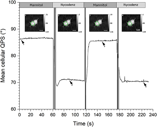
Figure 5. QPS stabilization time. Graph showing the mean cellular QPS of one HEK293T cell during the two-solution decoupling approach. The QPS is averaged over the cell body delineated by the green contour line, shown in the insets. The quantitative-phase images correspond to the time-points as defined by the respective arrowheads. Rectangles across the top illustrate the perfusion sequence of the mannitol- (dark gray) and Nycodenz-based (light gray) solutions. The mean cellular QPS as well as the color bars of the insets are expressed in degrees and the scale bars are 5 μm.

Experimentally, the typical ${\Delta \overline{\varphi }}_c$ fluctuations (on the scale of a few seconds), for which the automated segmentation algorithm is stable, are ~0.2°. Such phase fluctuations, although dependent on the coherent noise, result mainly from the natural cell micro-movements and deformations namely the cell-mediated noise [44]. Considering these cell body phase fluctuations, the typical time to obtain an appropriate ${\Delta \overline{\varphi }}_c$ stabilization, to perform a two-liquid decoupling procedure with the 3D-printed flow chamber, is ~10.09 ± 3.46 and 12.79 ± 3.57 s from mannitol to Nycodenz, and vice versa, respectively. This determination results from an extensive analysis of 37 turnovers, randomly positioned over the entire imaging slit of the four different sample holders. Compared to the originally reported ${\Delta \overline{\varphi }}_c$ stabilization time of 30–60 s for the mannitol-Nycodenz transition, this represents a reduction by at least a factor of three to six [16, 25]. The fabrication parameter having the most restrictive tolerance to obtain the reported performances on the washout process is the concentric alignment of the axes of the channels to insert the microtubes. This tolerance is met by the micrometric resolution of the 3D printer described in this paper. Although QP-DHM has coherent noise originating from the degree coherence of the light source required to perform off-axis interferometry, from experimental observations, there are no significant speckles originating specifically from the potential remaining roughness of the internal walls of the imaging slit.

Keeping the QPS stabilization time as short as possible is important considering that even more significant cell changes, including important cell position and shape modifications involving thickness and/or refractive index, are very likely to take place over time causing important artifacts on ${\overline{n}}_c$, ${\overline{h}}_c$ and V_c measurements. In general, the Nycodenz-mannitol QPS stabilization times are longer by a factor of ~1.3. In addition, the variability in the QPS stabilization time for a given pair of liquid is governed (for now) by the reproducibility of the fabrication process and aging of the sample holder. The rapidity of the QPS stabilization time is an indication of the homogeneity of the refractive index of the perfusion medium inside the imaging slit.

Thus, the presence of a steady-state and fully-developed laminar flow improves the washout process of the solutions resulting in a faster QPS stabilization time corresponding to the restauration of the known values n_m1or n_m2 of the two perfusion solutions. This makes the a priori knowledge of the refractive indices of the perfusion media a more reliable approximation than the one in situ. Moreover, a flow chamber with such a homogenous flow of fluid is well-suited to perform pharmacological experiments.

Measurements of the Whole-Cell Refractive Index and Absolute Cell Volume

As previously mentioned, the decoupling procedure measures the integral IRI over the OPL of each pixel ${\overline{n}}_c(x,y)$ and the corresponding cell thickness h_c(x, y) separately from Δϕ_c(x, y). Thanks to the mean value theorem for integrals, ${\int }_0^{h_c(x,y)}{n}_c(x,y,z)dz={\overline{n}}_c(x,y)h_c(x,y)$, such a cell thickness measurement remains valid even if ${\overline{n}}_c(x,y)$ exhibits some variations along the OPL of each pixel, as long as the observed sample is a weakly-scattering object such as a living cell, i.e., one that does not significantly deviate optical rays from their incident direction. However, as mentioned above, during the washout processes, both cell-mediated noise as well as coherent noise (contributing to the major part of the phase fluctuations), preclude the possibility to obtain a precise value for h_c(x, y) and ${\overline{n}}_c(x,y)$ measurements at the level of individual pixels. Nonetheless, the spatial phase averaging over a cell body [44] significantly decreases both effects leading to the precise measurement of ${\overline{n}}_c$ and ${\overline{h}}_c$, and consequently of V_c according to Equations (7)–(9). These biophysical parameters, along with their respective errors obtained by the technique of partial derivatives, were calculated for populations of three cell types in culture including primary neurons, HEK293T cells, and NIH3T3 cells.

The fluctuations of the mean cellular QPS ${\Delta \overline{\varphi }}_c$ represent the main factor limiting the precision of ${\overline{n}}_c$ and ${\overline{h}}_c$ measurements. Typical ${\Delta \overline{\varphi }}_c$ fluctuations of 0.2°, as seen in Figure 5, used in conjunction with the technique of partial derivatives on Equations (7)–(8) lead to values of $\delta {\overline{n}}_c$ = 0.0003 and ${\delta \overline{h}}_c$ = 70 nm. Such a high precision on ${\overline{n}}_c$ and ${\overline{h}}_c$ measurements comes at the price of losing the spatial resolution of these two biophysical parameters. Interestingly, $\delta {\overline{n}}_c$ and ${\delta \overline{h}}_c$, shown in Figure 6A, do not exhibit a significant decrease as a function of S_c. This is consistent with the fact that the main effect of the spatial averaging on the cell-mediated noise is already reached for surfaces ranging from 100 to 400 μm² [44]. Typically, across all the cells of the populations of the three cell types studied, the precisions at the single-cell level of ${\overline{n}}_c$ and ${\overline{h}}_c$ are 0.0006 and 100 nm, respectively. The measurements of V_c as a function of S_c are shown in Figure 7A. It is observed that the precision of V_c is drastically affected by S_c. This is detailed in Figure 6B presenting the absolute and relative errors of V_c as a function of S_c obtained with the technique of partial derivatives on Equation (9). While δV_c increases for large cellular surfaces, the relative error $\frac{\delta V_c}{V_c}$ decreases. According to Equation (9) and given the fact that ${\delta \overline{h}}_c$ does not significantly depend on S_c as shown in Figure 6A, it turns out that the influence of S_c on V_c should come from our capacity of measuring S_c with precision. This is consistently illustrated in Figure 6C showing the behavior of both δS_c and $\frac{\delta S_c}{S_c}$ as a function of S_c. Considering the SNR of ${\Delta \overline{\varphi }}_c$, it is understood that the precision of S_c is mainly limited by the lateral resolution of the quantitative-phase images dictated by the NA of the microscope objective, which is 0.7 in this case. Therefore, the decrease of $\frac{\delta S_c}{S_c}$ as a function of S_c reflects the ratio between the cell perimeter and its surface. The tendency of a behavior inversely proportional to the radius of the cell surface comes from the presence of a significant number of nearly round cells which is specially the case for the smallest cells of our populations. Figure 7B shows ${\overline{n}}_c$ as a function of V_c. Interestingly, this highlights the fact that cells with smaller V_c tend to have a higher ${\overline{n}}_c$. This observation is consistent with a ratio between the solid and the cytosolic portion, which is higher for smaller cells [54].

FIGURE 6

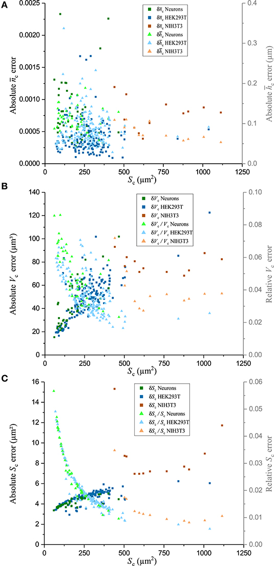
Figure 6. Error of biophysical measurements. Absolute and relative errors of numerous biophysical measurements as a function of S_c for three cell types in culture, including primary neurons, and HEK293T and NIH3T3 cells. Data points plotted with darker squares are in relation to the left axis and data points plotted with lighter shade triangles are in relation to the right axis. (A) Plots of the absolute ${\overline{n}}_c$ error (left) and absolute ${\overline{h}}_c$ error (right), (B) absolute (left) and relative (right) V_c error, and (C) absolute (left) and relative (right) S_c error.

FIGURE 7

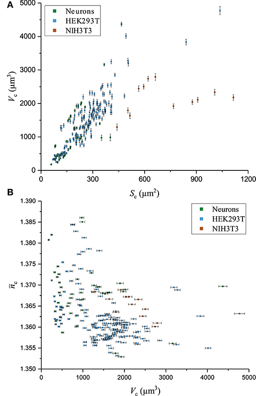
Figure 7. Biophysical parameters. Various biophysical measurements for three cell types in culture, including primary neurons, and HEK293T and NIH3T3 cells. (A) Graph of V_c as a function of S_c, (B) Scatter of ${\overline{n}}_c$ as a function of V_c.

Table 1 shows the means and the standard deviations of the distributions of a set of biophysical parameters measured over populations of the three different cell types studied. Mean values and standard deviations, for cell populations, of whole-cell refractive index $\overline{n}$ and average cell thickness $\overline{h}$ of 1.3672 ± 0.0070 and 5.87 ± 2.38 μm for neurons (n = 64), 1.3637 ± 0.0086 and 5.27 ± 1.46 μm for HEK293T cells (n = 202), 1.3660 ± 0.0038 and 3.01 ± 0.96 μm for NIH3T3 cells (n = 14) were obtained, respectively, for resting state. Mean values and standard deviations, for cell populations, of absolute cell volumes V of 1,210 ± 890, 1,460 ± 840, and 2,200 ± 480 μm³ were obtained for the populations of neurons, and HEK293T and NIH3T3 cells, respectively. The standard deviations reported in Table 1 relate to the spread of the distribution of the different biophysical parameters, reflecting the heterogeneity across the cell populations of a given cell type and not the precision of a single-cell measurement. Interestingly, in the conditions of cell culture used here, NIH3T3 cells are thinner by a factor of two, but have greater V because of their larger S_c. In addition, it seems that the distribution of $\overline{n}$ is rather narrow while for V it is much broader. It is interesting to note that the absolute values of the cell biophysical parameters presented here are consistent with existing literature, even when considering various measurement techniques [26, 29, 36, 55].

TABLE 1

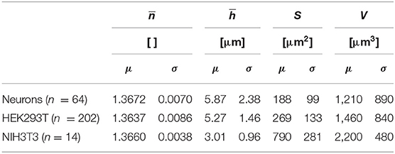
Table 1. Measured biophysical parameters on populations of primary neurons, HEK293T, and NIH3T3 cells during their resting state.

Osmotic Challenges

The membranes of animal cells are highly permeable to water. Water movement across membranes is in large part dictated by osmotic pressure gradients. During a hypo-osmotic challenge, a net water influx occurs, causing a cellular swelling. On the contrary, in a hyper-osmotic challenge, there is a water efflux, leading to cell shrinkage. Changing the osmolarity of the extracellular medium to perform osmotic challenges implies the use of at least two solutions, a number that is doubled in the case of assessing both ${\overline{n}}_c$ as well as V_c through the two-liquid decoupling approach. Therefore, these experiments offer an excellent paradigm to confirm the efficiency and performance of the proposed flow chamber.

The responses of two cell types in culture (namely the neurons and HEK293T cells), to osmotic challenges, have been studied. First, a typical response of the mean cellular QPS (black solid line) for a HEK293T cell during a hypo-osmotic challenge is shown in Figure 8. The mean cellular QPS results from an averaging performed over the cell body delineated by the green contour lines, ${\Delta \overline{\varphi }}_c$, as shown in insets. These quantitative-phase images correspond to the time-points defined by the arrowheads. Rectangles on the top illustrate the perfusion sequence of the various perfusion solutions, namely the iso-osmotic mannitol (blue), iso-osmotic Nycodenz (red), hypo-osmotic Nycodenz (light red), and hypo-osmotic mannitol (light blue). As described in Section Two-Liquid Decoupling Approach, the strength and duration of the hypo-osmotic stress are 50 mOsm and 5 min, respectively. The vertical gray dashed line illustrates the onset of the hypo-osmotic challenge.

FIGURE 8

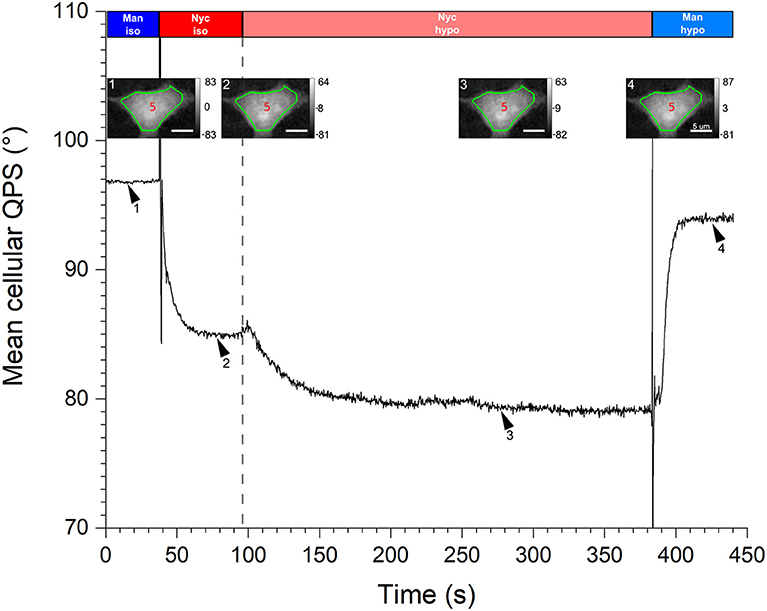
Figure 8. Hypo-osmotic challenge. A graph of the mean cellular QPS of one HEK293T cell during a hypo-osmotic challenge is shown. The QPS is averaged over the cell body delineated by the green contour line, shown in the insets. The quantitative-phase images correspond to the time-points defined by the respective arrowheads. Rectangles across the top illustrate the perfusion sequence of the various solutions, namely the iso-osmotic mannitol (blue), iso-osmotic Nycodenz (red), hypo-osmotic Nycodenz (light red), and hypo-osmotic mannitol (light blue). The vertical gray dashed line indicates the onset of the hypo-osmotic challenge. The mean cellular QPS as well as the color bars of the insets are expressed in degrees and the scale bars are 5 μm.

As discussed in Section Quantitative-Phase Signal Stabilization Time, the first two plateaus of ${\Delta \overline{\varphi }}_c$ are used to obtain the ${\overline{n}}_c$ and ${\overline{h}}_c$ values during the cell resting state; in this specific case their values are 1.3737 ± 0.0007 and 4.50 ± 0.12 μm, respectively. This given ${\overline{h}}_c$, used in conjunction with the corresponding S_c of 247 ± 5 μm², translate to a V_c of 1,110 ± 30 μm³. As soon as the hypo-osmotic Nycodenz solution is perfused, ${\Delta \overline{\varphi }}_c$ is rapidly decreased to finally reach a stabilized state after around 60 s of challenge, corresponding to an equilibrium between intra- and extra-cellular osmotic pressures. Next, the perfusion of the hypo-osmotic mannitol medium leads to the fourth ${\Delta \overline{\varphi }}_c$ plateau. These last two plateaus of ${\Delta \overline{\varphi }}_c$ are used to calculate ${\overline{n}}_c$ = 1.3670 ± 0.0006 and ${\overline{h}}_c$ = 5.26 ± 0.11 μm values corresponding to the new steady-state induced by the hypo-osmotic challenge, namely a cellular swelling. For this particular cell, the hypo-osmotic challenge effectively mediated a decrease of ${\overline{n}}_c$, given by ${\Delta \overline{n}}_c={\overline{n}}_{c_{hypo}}-{\overline{n}}_c$ = −0.007 ± 0.001, and an increase of ${\overline{h}}_c$, corresponding to ${\Delta \overline{h}}_c={\overline{h}}_{c_{hypo}}-{\overline{h}}_c$ = 0.8 ± 0.2 μm. The hypo-osmotic challenge caused a cell volume increase of ΔV_c = V_chypo−V_c = 190 ± 70 μm³ and a swelling factor β = V_chypo/V_c = 1.17 ± 0.06.

For a hyper-osmotic challenge, the experiment is virtually the same as in Figure 8 except that the two last perfusion media were different, namely hyper-osmotic Nycodenz and hyper-osmotic mannitol. Similarly, biophysical data are obtained from the values of the different plateaus of ${\Delta \overline{\varphi }}_c$. In summary, Table 2 shows the hypo-osmotic and hyper-osmotic induced changes of a set of biophysical parameters expressed as the mean value and standard deviation calculated over population of two cell types in culture, including neurons (n = 16 and n = 9, respectively) and HEK293T cells (n = 16 and n = 25, respectively). Here also, the standard deviations reported in Table 2 relate to the range of the values of the different biophysical parameters, reflecting the heterogeneity across the cell population of a given cell type and not the precision of a single-cell measurement.

TABLE 2

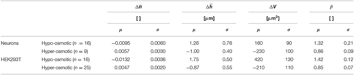
Table 2. Measured variations of biophysical parameters induced by osmotic challenges on populations of primary neurons and HEK293T cells.

The data presented in Table 2 suggests that the biophysical parameter $\Delta \overline{n}$ is sufficient to quantify water movements over a cell population. The hypo-osmotic challenge induces a decrease of $\overline{n}$ at the level of a population of cells. This reduction is consistent with a hypo-osmotic water influx, resulting in a dilution of the intracellular protein concentration—the cellular component that largely determines the value of ${\overline{n}}_c$. The contradictory fall of ${\Delta \overline{\varphi }}_c$ results from a lateral dilution of the dry mass concentration. The explanation is also valid for the case of a hyper-osmotic challenge. In addition, both the $\Delta \overline{n}$ and the ΔV as well as the β values obtained here are consistent with the existing literature [26, 27, 29]. The measurements of these biophysical data for both osmotic conditions reinforce our understanding of the cellular mechanisms of these phenomena.

Conclusion

In conclusion, a low-cost, open-source, and do-it-yourself 3D-printed flow chamber optimized to efficiently perform dissociated measurements of ${\overline{n}}_c$ and ${\overline{h}}_c$, resulting in accurate calculations of the critical cell parameter V_c with QP-DHM and with QPI in a more general manner, has been developed. The flow chamber has been 3D-printed with a plastic filament for which the raw material itself is biocompatible. The entire flow chamber costs <12 USD to fabricate, of which a mere 0.86 USD is for the plastic itself. The compatibility of the flow chamber with live cell imaging has been demonstrated by quantifying its cell viability rate when compared to a control condition. The assay revealed similar cell viability rates in both conditions, namely 81.71 ± 4.91% for the flow chamber and 84.74 ± 2.26% for the control condition. The geometry of the flow chamber has been customized to have a steady-state and fully-developed laminar flow which optimizes the washout process. The presence of such a flow of fluid inside the imaging slit has been verified both numerically and experimentally. Specifically, following the two-liquid decoupling sequence, a state where the refractive index of the solution is homogeneously distributed over the entire imaging slit can be rapidly obtained. This can be assessed by experimentally measuring the time to obtain a stabilized QPS. The mean QPS stabilization time of 37 turnovers resulting from four different sample holders has been quantified and found to be 10.09 ± 3.46 and 12.79 ± 3.57 s, depending on the given sequence of liquids used. Such a washout optimization has permitted to measure with high reliability the important cell biophysical parameters including ${\overline{n}}_c$, ${\overline{h}}_c$, and V_c and results in a faster stabilization time, thereby resulting in reduced cell changes and the resulting artifacts. For a typical cell body having a V_c of 1,250 μm³ and a S_c of 300 μm², ${\overline{n}}_c$, ${\overline{h}}_c$, and V_c values are usually measured with a precision of 0.0006, 100 nm, and 50 μm³, respectively. Furthermore, the variations of ${\overline{n}}_c$, ${\overline{h}}_c$, and V_c have been quantitatively calculated during hypo-osmotic and hyper-osmotic challenges. Hypo-osmotic challenges of 50 mOsm on cell populations have shown globally a dilution of $\overline{n}$, on an average of −0.0115, as well as an increase of $\overline{h}$, typically of 1.50 μm, and a gain of V, characteristically of 290 μm³. As expected, changes in the opposite directions, reflecting a reversible process, have been observed in the case of hyper-osmotic challenges. Finally, the design files of the do-it-yourself flow chamber will be shared with the scientific community through an open-source model for rapid dissemination and maximum impact.

Data Availability Statement

The raw data supporting the conclusions of this manuscript will be made available by the authors, without undue reservation, to any qualified researcher.

Author Contributions

EB and PM designed the study, wrote the paper with help from SL, ÉR-P and PL, and co-supervised the research. SL, ÉR-P, and PL conducted experiments. SL and PL processed the data. ÉR-P analyzed the data.

Funding

This work was supported by the Natural Sciences and Engineering Research Council of Canada (NSERC) (RGPIN-2018-06198), the Canada Excellence Research Chairs (CERC) program and the Canada Foundation for Innovation (CFI) (36689, 34265).

Conflict of Interest

PM declares the presence of a potential conflict of interest as a co-founder of Lyncée Tec, a company that commercializes digital holographic microscopes. However, the study has been performed independently of Lyncée Tec in academic laboratories.

The remaining authors declare that the research was conducted in the absence of any commercial or financial relationships that could be construed as a potential conflict of interest.

Acknowledgments

The authors would like to acknowledge the contribution all former interns and staff members, namely Gabriel Anctil, Vincent Roy, Alyson Bernatchez, Valerie Watters, Anne-Sophie Poulin-Girard, Chloé Martel, Jean-Michel Mugnes, and Jean-Xavier Giroux for their contribution in the development of the flow chamber and post-processing of quantitative-phase images. The authors would also like to acknowledge the services of CMC Microsystems which facilitated this research.

References

1. Lang F, Busch GL, Ritter M, Völkl H, Waldegger S, Gulbins E, et al. Functional significance of cell volume regulatory mechanisms. Physiol Rev. (1998) 78:247–306. doi: 10.1152/physrev.1998.78.1.247

PubMed Abstract | CrossRef Full Text | Google Scholar

2. Hoffmann EK, Lambert IH, Pedersen SF. Physiology of cell volume regulation in vertebrates. Physiol Rev. (2009) 89:193–277. doi: 10.1152/physrev.00037.2007

PubMed Abstract | CrossRef Full Text | Google Scholar

3. Waldegger S, Lang F. Cell volume and gene expression. J Membr Biol. (1998) 162:95–100. doi: 10.1007/s002329900346

PubMed Abstract | CrossRef Full Text | Google Scholar

4. Lang F, Ritter M, Gamper N, Huber S, Fillon S, Tanneur V, et al. Cell volume in the regulation of cell proliferation and apoptotic cell death. Cell Physiol Biochem. (2000) 10:417–28. doi: 10.1159/000016367

PubMed Abstract | CrossRef Full Text | Google Scholar

5. McManus ML, Churchwell KB, Strange K. Regulation of cell volume in health and disease. N Engl J Med. (1995) 333:1260–7. doi: 10.1056/NEJM199511093331906

PubMed Abstract | CrossRef Full Text | Google Scholar

6. Model MA. Methods for cell volume measurement. Cytom A. (2018) 93:281–96. doi: 10.1002/cyto.a.23152

PubMed Abstract | CrossRef Full Text | Google Scholar

7. Tzur A, Moore JK, Jorgensen P, Shapiro HM, Kirschner MW. Optimizing optical flow cytometry for cell volume-based sorting and analysis. PLoS ONE. (2011) 6:1–9. doi: 10.1371/journal.pone.0016053

PubMed Abstract | CrossRef Full Text | Google Scholar

8. Gregg JL, McGuire KM, Focht DC, Model MA. Measurement of the thickness and volume of adherent cells using transmission-through-dye microscopy. Pflugers Arch Eur J Physiol. (2010) 460:1097–104. doi: 10.1007/s00424-010-0869-2

PubMed Abstract | CrossRef Full Text | Google Scholar

9. Gray ML, Hoffman RA, Hansen WP. A new method for cell volume measurement based on volume exclusion of a fluorescent dye. Cytometry. (1983) 3:428–34. doi: 10.1002/cyto.990030607

PubMed Abstract | CrossRef Full Text | Google Scholar

10. Marquet P, Depeursinge C, Magistretti PJ. Exploring neural cell dynamics with digital holographic microscopy. Annu Rev Biomed Eng. (2013) 15:407–31. doi: 10.1146/annurev-bioeng-071812-152356

PubMed Abstract | CrossRef Full Text | Google Scholar

11. Park Y, Depeursinge C, Popescu G. Quantitative phase imaging in biomedicine. Nat Photonics. (2018) 12:578–89. doi: 10.1038/s41566-018-0253-x

CrossRef Full Text | Google Scholar

12. Marquet P, Rappaz B, Magistretti PJ, Cuche E, Emery Y, Colomb T, et al. Digital holographic microscopy: a noninvasive contrast imaging technique allowing quantitative visualization of living cells with subwavelength axial accuracy. Opt Lett. (2005) 30:468–70. doi: 10.1364/OL.30.000468

PubMed Abstract | CrossRef Full Text | Google Scholar

13. Popescu G, Ikeda T, Dasari RR, Feld MS. Diffraction phase microscopy for quantifying cell structure and dynamics. Opt Lett. (2006) 31:775–7. doi: 10.1364/OL.31.000775

PubMed Abstract | CrossRef Full Text | Google Scholar

14. Kemper B, von Bally G. Digital holographic microscopy for live cell applications and technical inspection. Appl Opt. (2008) 47:A52–61. doi: 10.1364/AO.47.000A52

PubMed Abstract | CrossRef Full Text | Google Scholar

15. Bon P, Maucort G, Wattellier B, Monneret S. Quadriwave lateral shearing interferometry for quantitative phase microscopy of living cells. Opt Express. (2009) 17:13080–94. doi: 10.1364/OE.17.013080

PubMed Abstract | CrossRef Full Text | Google Scholar

16. Moon I, Jaferzadeh K, Ahmadzadeh E, Javidi B. Automated quantitative analysis of multiple cardiomyocytes at the single-cell level with three-dimensional holographic imaging informatics. J Biophotonics. (2018) 11:e201800116. doi: 10.1002/jbio.201800116

PubMed Abstract | CrossRef Full Text | Google Scholar

17. Chmelik R, Krizova A, Kollarova V, Vesely P, Collakova J, Slaba M, et al. Coherence-controlled holographic microscopy enabled recognition of necrosis as the mechanism of cancer cells death after exposure to cytopathic turbid emulsion. J Biomed Opt. (2015) 20:111213. doi: 10.1117/1.JBO.20.11.111213

PubMed Abstract | CrossRef Full Text | Google Scholar

18. Barer R. Refractometry and interferometry of living cells. J Opt Soc Am. (1957) 47:545. doi: 10.1364/JOSA.47.000545

PubMed Abstract | CrossRef Full Text | Google Scholar

19. Zicha D, Dunn GA. An image processing system for cell behaviour studies in subconfluent cultures. J Microsc. (1995) 179:11–21. doi: 10.1111/j.1365-2818.1995.tb03609.x

CrossRef Full Text | Google Scholar

20. Popescu G, Park Y, Lue N, Best-Popescu C, Deflores L, Dasari RR, et al. Optical imaging of cell mass and growth dynamics. Am J Physiol Physiol. (2008) 295:C538–44. doi: 10.1152/ajpcell.00121.2008

PubMed Abstract | CrossRef Full Text | Google Scholar

21. Rappaz B, Cano E, Colomb T, Kühn J, Depeursinge C, Simanis V, et al. Noninvasive characterization of the fission yeast cell cycle by monitoring dry mass with digital holographic microscopy. J Biomed Opt. (2009) 14:034049. doi: 10.1117/1.3147385

PubMed Abstract | CrossRef Full Text | Google Scholar

22. Fu D, Choi W, Sung Y, Yaqoob Z, Dasari RR, Feld M. Quantitative dispersion microscopy. Biomed Opt Express. (2010) 1:347–53. doi: 10.1364/BOE.1.000347

PubMed Abstract | CrossRef Full Text | Google Scholar

23. Rappaz B, Barbul A, Hoffmann A, Boss D, Korenstein R, Depeursinge C, et al. Spatial analysis of erythrocyte membrane fluctuations by digital holographic microscopy. Blood Cell Mol Dis. (2009) 42:228–32. doi: 10.1016/j.bcmd.2009.01.018

PubMed Abstract | CrossRef Full Text | Google Scholar

24. Boss D, Hoffmann A, Rappaz B, Depeursinge C, Magistretti PJ, Van de Ville D, et al. Spatially-resolved eigenmode decomposition of red blood cells membrane fluctuations questions the role of ATP in flickering. PLoS ONE. (2012) 7:e40667. doi: 10.1371/journal.pone.0040667

PubMed Abstract | CrossRef Full Text | Google Scholar

25. Javidi B, Markman A, Rawat S, O'Connor T, Anand A, Andemariam B. Sickle cell disease diagnosis based on spatio-temporal cell dynamics analysis using 3D printed shearing digital holographic microscopy. Opt Express. (2018) 26:13614–27. doi: 10.1364/OE.26.013614

PubMed Abstract | CrossRef Full Text | Google Scholar

26. Rappaz B, Marquet P, Cuche E, Emery Y, Depeursinge C, Magistretti PJ. Measurement of the integral refractive index and dynamic cell morphometry of living cells with digital holographic microscopy. Opt Express. (2005) 13:9361–73. doi: 10.1364/OPEX.13.009361

PubMed Abstract | CrossRef Full Text | Google Scholar

27. Curl CL, Bellair CJ, Harris PJ, Allman BE, Roberts A, Nugent KA, et al. Single cell volume measurement by quantitative phase microscopy (QPM): a case study of erythrocyte morphology. Cell Physiol Biochem. (2006) 17:193–200. doi: 10.1159/000094124

PubMed Abstract | CrossRef Full Text | Google Scholar

28. Rappaz B, Barbul A, Emery Y, Korenstein R, Depeursinge C, Magistretti PJ, et al. Comparative study of human erythrocytes by digital holographic microscopy, confocal microscopy, and impedance volume analyzer. Cytom A. (2008) 73:895–903. doi: 10.1002/cyto.a.20605

PubMed Abstract | CrossRef Full Text | Google Scholar

29. Boss D, Kühn J, Jourdain P, Depeursinge C, Magistretti PJ, Marquet P. Measurement of absolute cell volume, osmotic membrane water permeability, and refractive index of transmembrane water and solute flux by digital holographic microscopy. J Biomed Opt. (2013) 18:036007. doi: 10.1117/1.JBO.18.3.036007

PubMed Abstract | CrossRef Full Text | Google Scholar

30. Jourdain P, Allaman I, Rothenfusser K, Fiumelli H, Marquet P, Magistretti PJ. L-Lactate protects neurons against excitotoxicity: implication of an ATP-mediated signaling cascade. Sci Rep. (2016) 6:21250. doi: 10.1038/srep21250

PubMed Abstract | CrossRef Full Text | Google Scholar

31. Jourdain P, Becq F, Lengacher S, Boinot C, Magistretti PJ, Marquet P. The human CFTR protein expressed in CHO cells activates aquaporin-3 in a cAMP-dependent pathway: study by digital holographic microscopy. J Cell Sci. (2014) 127:546–56. doi: 10.1242/jcs.133629

PubMed Abstract | CrossRef Full Text | Google Scholar

32. Jourdain P, Boss D, Rappaz B, Moratal C, Hernandez MC, Depeursinge C, et al. Simultaneous optical recording in multiple cells by digital holographic microscopy of chloride current associated to activation of the ligand-gated chloride channel GABAA receptor. PLoS ONE. (2012) 7:e51041. doi: 10.1371/journal.pone.0051041

CrossRef Full Text | Google Scholar

33. Jourdain P, Pavillon N, Moratal C, Boss D, Rappaz B, Depeursinge C, et al. Determination of transmembrane water fluxes in neurons elicited by glutamate ionotropic receptors and by the cotransporters KCC2 and NKCC1: a digital holographic microscopy study. J Neurosci. (2011) 31:11846–54. doi: 10.1523/JNEUROSCI.0286-11.2011

PubMed Abstract | CrossRef Full Text | Google Scholar

34. Cotte Y, Toy F, Jourdain P, Pavillon N, Boss D, Magistretti P, et al. Marker-free phase nanoscopy. Nat Photonics. (2013) 7:113–7. doi: 10.1038/nphoton.2012.329

CrossRef Full Text | Google Scholar

35. Yang SA, Yoon J, Kim K, Park YK. Measurements of morphological and biophysical alterations in individual neuron cells associated with early neurotoxic effects in Parkinson's disease. Cytom A. (2017) 91:510–8. doi: 10.1002/cyto.a.23110

PubMed Abstract | CrossRef Full Text | Google Scholar

36. Curl CL, Bellair CJ, Harris T, Allman BE, Harris PJ, Stewart AG, et al. Refractive index measurement in viable cells using quantitative phase-amplitude microscopy and confocal microscopy. Cytom A. (2005) 65:88–92. doi: 10.1002/cyto.a.20134

PubMed Abstract | CrossRef Full Text | Google Scholar

37. Kemper B, Carl D, Schnekenburger J, Bredebusch I, Schafer M, Domschke W, et al. Investigation of living pancreas tumor cells by digital holographic microscopy. J Biomed Opt. (2006) 11:034005. doi: 10.1117/1.2204609

PubMed Abstract | CrossRef Full Text | Google Scholar

38. Lue N, Popescu G, Ikeda T, Dasari RR, Badizadegan K, Feld MS. Live cell refractometry using microfluidic devices. Opt Lett. (2006) 31:2759–61. doi: 10.1364/OL.31.002759

PubMed Abstract | CrossRef Full Text | Google Scholar

39. Kemper B, Kosmeier S, Langehanenberg P, von Bally G, Bredebusch I, Domschke W, et al. Integral refractive index determination of living suspension cells by multifocus digital holographic phase contrast microscopy. J Biomed Opt. (2007) 12:054009. doi: 10.1117/1.2798639

PubMed Abstract | CrossRef Full Text | Google Scholar

40. Rappaz B, Charrière F, Depeursinge C, Magistretti PJ, Marquet P. Simultaneous cell morphometry and refractive index measurement with dual-wavelength digital holographic microscopy and dye-enhanced dispersion of perfusion medium. Opt Lett. (2008) 33:744–6. doi: 10.1364/OL.33.000744

PubMed Abstract | CrossRef Full Text | Google Scholar

41. Przibilla S, Dartmann S, Vollmer A, Ketelhut S, Greve B, von Bally G, et al. Sensing dynamic cytoplasm refractive index changes of adherent cells with quantitative phase microscopy using incorporated microspheres as optical probes. J Biomed Opt. (2012) 17:0970011. doi: 10.1117/1.JBO.17.9.097001

PubMed Abstract | CrossRef Full Text | Google Scholar

42. Dardikman G, Nygate YN, Barnea I, Turko NA, Singh G, Javidi B, et al. Integral refractive index imaging of flowing cell nuclei using quantitative phase microscopy combined with fluorescence microscopy. Biomed Opt Express. (2018) 9:88–92. doi: 10.1364/BOE.9.001177

PubMed Abstract | CrossRef Full Text | Google Scholar

43. Przybytek A, Gubanska I, Kucinska-Lipka J, Janik H. Polyurethanes as a potential medical-grade filament for use in fused deposition modeling 3D printers – a brief review. Fibres Text East Eur. (2018) 6:120–5. doi: 10.5604/01.3001.0012.5168

CrossRef Full Text | Google Scholar

44. Lévesque SA, Mugnes JM, Bélanger E, Marquet P. Sample and substrate preparation for exploring living neurons in culture with quantitative-phase imaging. Methods. (2018) 136:90–107. doi: 10.1016/j.ymeth.2018.02.001

PubMed Abstract | CrossRef Full Text | Google Scholar

45. Dardikman G, Shaked NT. Review on methods of solving the refractive index–thickness coupling problem in digital holographic microscopy of biological cells. Opt Commun. (2018) 422:8–16. doi: 10.1016/j.optcom.2017.11.084

CrossRef Full Text | Google Scholar

46. Bélanger E, Lévesque SA, Anctil G, Poulin-Girard A-S, Marquet P. Low-cost production and sealing procedure of mechanical parts of a versatile 3D-printed perfusion chamber for digital holographic microscopy of primary neurons in culture. In: Proceedings SPIE 10074, Quantitative Phase Imaging III. San Francisco, CA (2017). p. 100741S. doi: 10.1117/12.2253036

CrossRef Full Text | Google Scholar

47. Tinevez JY, Perry N, Schindelin J, Hoopes GM, Reynolds GD, Laplantine E, et al. TrackMate: an open and extensible platform for single-particle tracking. Methods. (2017) 115:80–90. doi: 10.1016/j.ymeth.2016.09.016

PubMed Abstract | CrossRef Full Text | Google Scholar

48. Nault F, De Koninck P. Dissociated hippocampal cultures. In: Doering LC, editor. Protocols 799 for Neural Cell Culture. Totowa, NJ: Humana Press (2009). p. 137–59. doi: 10.1007/978-1-60761-292-6_8

CrossRef Full Text | Google Scholar

49. Cuche E, Marquet P, Depeursinge C. Simultaneous amplitude-contrast and quantitative phase-contrast microscopy by numerical reconstruction of Fresnel off-axis holograms. Appl Opt. (1999) 38:6994–7001. doi: 10.1364/AO.38.006994

PubMed Abstract | CrossRef Full Text | Google Scholar

50. Cuche E, Marquet P, Depeursinge C. Spatial filtering for zero-order and twin-image elimination in digital off-axis holography. Appl Opt. (2000) 39:4070–5. doi: 10.1364/AO.39.004070

PubMed Abstract | CrossRef Full Text | Google Scholar

51. Colomb T, Kühn J, Charrière F, Depeursinge C, Marquet P, Aspert N. Total aberrations compensation in digital holographic microscopy with a reference conjugated hologram. Opt Express. (2006) 14:4300–6. doi: 10.1364/OE.14.004300

PubMed Abstract | CrossRef Full Text | Google Scholar

52. Colomb T, Cuche E, Charrière F, Kühn J, Aspert N, Montfort F, et al. Automatic procedure for aberration compensation in digital holographic microscopy and applications to specimen shape compensation. Appl Opt. (2006) 45:851–63. doi: 10.1364/AO.45.000851

PubMed Abstract | CrossRef Full Text | Google Scholar

53. Munson BR, Young DF, Okiishi TH, Huebsch WW. Fundamentals of Fluid Mechanics. 6th ed. Hoboken, NJ: Wiley (2009).

Google Scholar

54. Olsen H, Kinne-Saffran E, Kinne RKH, Wehner F, Tinel H. Cell volume regulation: osmolytes, osmolyte transport, and signal transduction. Rev Physiol Biochem Pharmacol. (2003) 148:1–80. doi: 10.1007/s10254-003-0009-x

PubMed Abstract | CrossRef Full Text | Google Scholar

55. Liu PY, Chin LK, Ser W, Chen HF, Hsieh CM, Lee CH, et al. Cell refractive index for cell biology and disease diagnosis: past, present and future. Lab Chip. (2016) 16:634–44. doi: 10.1039/C5LC01445J

PubMed Abstract | CrossRef Full Text | Google Scholar

Appendix A

Flow Chamber Fabrication Protocol

Fabrication of the Lid and Base

• Slice .stl files produced with SolidWorks of the lid and base in Cura, flat face down on the print bed.

◦ Use 0.4 mm nozzle and 30% infill

• Print with Taulman3D Guideline and remove from print bed.

• Glue magnets in the 4 slots of both parts.

◦ Make sure all magnets placed in the lid have inverted polarities to those placed in the base.

• Wait for the glue to dry.

Fabrication of the Sample Holder

• Slice sample holder .stl file produced with SolidWorks in Cura, flat face down on the print bed.

◦ Use 0.25 mm nozzle and full infill

◦ Use custom settings to increase infill overlap percentage to 30%

■ This setting can be added via: Preferences - > Settings - > Infill

◦ Reduce print speed to 30 mm/s

◦ Add brim for better adhesion to the print bed

• Change nozzle on printer to 0.25 mm and precisely calibrate the glass print bed.

• Print with Taulman3D Guideline using their recommendation for nozzle and bed temperatures.

• Wait for the bed to cool almost completely to remove.

• Cut micro-tubes to have two segments of ~2.5 cm.

◦ With small gage wire, verify the openings of the microtube segments.

• Glue micro-tubes in slots on each side of the sample holder.

◦ To prevent closing the tubes with the glue, pass small gage wire through them during the procedure.

• Wait for glue to dry.

• Treat with acetone as described in the reference of the main text.

• Press top coverslip on the sample holder directly after acetone treatment.

◦ The top of the holder can be distinguished by its small round indentation.

◦ This coverslip might break or fall during extensive use and should be replaced. This replacement can be greased upon the surface around the slit.

• Mount the flow chamber and test water tightness. The steps to mount the chamber are described in the next section (use clean coverslip instead of cell culture).

Mounting the Chamber With Cell Cultures

• Position the holder with the flattest face upwards.

• Slowly fill the channel with cell or perfusion medium. This will prevent the cells from dying when the coverslip is added.

• Place coverslip with cells on the sample holder.

• Clean off excess cell medium.

• Press the parafilm gasket onto the coverslip and holder, and make sure it sticks to the surface.

• Place sample holder in the base.

Place the lid slowly to avoid breaking the coverslips with the force of the magnets.