Investigation of Electromagnetic Wave Structures for a Coupled Model in Anti-ferromagnetic Spin Ladder Medium

1. Introduction

The theory of solitons is an attractive and exciting area of research. It is interlinked with many branches of mathematics and engineering [1–9]. Its aspects are charming and amazing because soliton travels with a steady speed and maintains its shape while propagating. It arises by balancing dispersive and non-linear terms. Solitons are discussed in different fields, and for references see [10–18].

The magnetic moments of molecules and atoms, normally linked to the spins of electrons, adjusted in an ordinary pattern with neighboring spins spell in reverse directions. This is like ferrimagnetism and ferromagnetism, a manifestation of ordered magnetism. Theoretical and mathematical theories argue that the spin ladder system is an excellent medium through which the interaction between different spins can be mapped to an approximate Heisinberg-type coupling with a coupling parameter that is inversely proportional to the distance between two separated spins. The dynamics of electromagnetic solitons with the coupled model in an anti-ferromagnetic spin ladder medium is of great interest among researchers due to its variety of applications. The spin ladder systems are a great source with which to develop significant interest in both experimental and theoretical points of view. Anti-ferromagnets test different ideas that involve a strong correlated system [6–9]. Spin ladders have many applications in different fields of quark physics, superconductors, and ultra-cold atoms, etc. The study of anti-ferromagnetic is still in its early stages. In anti-ferromagnets, the staggered magnetization variable M contributes the first derivative in this manner, i.e., (∇M). This is because, in the case of anti-ferromagnets, we have taken limits in specified intervals for two different sublattices individually. The parent cuprate insulators are the best example of anti-ferromagnets with isotropic and predominantly nearest-neighbor coupling. They satisfied the theory that gives an ordered ground state for $(s=\frac{1}{2}AF)$ by showing simple long range anti-ferromagnetic order at low temperature [19–26].

In this article, a coupled generalized derivative non-linear Schrödinger that describes the dynamical behavior of electromagnetic waves in a spin ladder antiferromagnetic medium system is considered and under investigation. The Heisenberg model was studied in Chen et al. [15] and Xu et al. [16] and considered with an anisotropic spin ladder and two ferromagnetic lattices. This lattices consist of N spins and are directed in the same direction? For more details see also Kavitha et al. [26]. The system is read as

$\begin{array}{l}i\frac{\partial q_j}{\partial t}+\frac{{\partial }^2{q}_j}{\partial x^2}+i{\alpha }_1\frac{\partial }{\partial x}(|q_j{|}^2{q}_j)-{\alpha }_2\frac{{\partial }^3{q}_j}{\partial x^3}+{\alpha }_3\frac{\partial }{\partial x}(q_n-q_j)\\ +{\alpha }_4\frac{{\partial }^3{q}_n}{\partial x^3}-{\alpha }_5\frac{\partial q_j}{\partial x}=0,& (1.1)\end{array}$

where q_j for j = 1, 2, and n = 3 − j, are the wave profiles, and α_k for k = 1, 2, ⋯ , 5, represent the real coefficients and are defined by ${\alpha }_1=\frac{1+g}{2g{M}_0^2}\alpha$, ${\alpha }_2=\frac{i{j}_a{\alpha }^3}{g\gamma }$, ${\alpha }_3=\frac{i{j}_b\alpha }{g\gamma }$, ${\alpha }_4=\frac{i{j}_c{\alpha }^3}{g\gamma }$ and ${\alpha }_5=\frac{iA}{g\gamma }\alpha$. Where j_a is ferromagnetic spin exchange interaction, j_b is antiferromagnetic coupling, j_c is the exchange coupling, and A represents the single-ion uniaxial anisotropy. The last equation is reduced to generalized coupled derivative non-linear Schrodinger system by considering α_m = 0, for m = 2, ⋯ , 5. In the following section, the considered model is analyzed.

2. The Modified Direct Algebraic Method

The section studies, MDAM [27] to investigate the wave structures of NLPDs. Thus, we consider NLPDs in following form:

$\begin{array}{l}H(q,q_t,q_x,q_{tx},q_{xx},\cdots )=0,\end{array}$

where q is a profile of wave structure and H is called a polynomial of q and its partial derivatives along with non-linear terms.

To extract wave structures, the method is followed by using the steps as discussed under.

Step 1: First, the NPDEs is converted into non-linear ODEs using the following transformation.

$\begin{array}{l}q(x,t)=U(\xi ),\text{and }\xi =B(x-wt),\end{array}$

where B and w are arbitrary parameters. It allows us to reduce the above equation in an ODE of U and have the form

$\begin{array}{l}Q(U,U^{\prime },U^{″},U^{‴},\cdots )=0.\end{array}$

Step 2: It is supposed that the solution of above equation satisfies the following ansatze:

$\begin{array}{l}U(\xi )=A_0+{\displaystyle \sum _{j=0}^m}{(A_j{\phi }^j+B_j{\phi }^{-j})}^i,\\ {\phi }^{\prime }=\gamma +{\phi }^2,\end{array}$

where γ is a parameter and its value is determined, $\phi =\phi (\xi ),{\phi }^{\prime }=\frac{d\phi }{d\xi }$.

Step 3: The homogeneous balance technique is followed where the highest order derivative is balanced with non-linear terms, to find the value of m, and where m ∈ Z₊.

Step 4: The use of the above equation and collecting the terms of the same order of φ^j together. Equate each term of φ^j to zero, which produce the system of algebraic equations.

Step 5: The solution of the system of algebraic equations along with the following wave structures are general solutions.

(i) If γ < 0

$\begin{array}{l}\phi =-\sqrt{-\gamma }tanh(\sqrt{-\gamma }\xi ),or\phi =-\sqrt{-\gamma }coth(\sqrt{-\gamma }\xi ),\end{array}$

it depends on condition.

(ii) If γ > 0

$\begin{array}{l}\phi =\sqrt{\gamma }tan(\sqrt{\gamma }\xi ),or\phi =-\sqrt{\gamma }cot(\sqrt{\gamma }\xi ),\end{array}$

it depends on condition.

(iii) If γ = 0

$\begin{array}{l}\phi =\frac{-1}{\xi }.\end{array}$

In the following section, the exact wave structures of Equation (1.1) can be obtained.

3. Analytical Analysis

We consider the complex transformation $q_j(x,t)=U_j(\xi )\times e^{i\varphi }$, where ξ = B(x − νt) and ϕ = −kx + wt + θ. It reduces the partial differential equation to an ordinary differential equation. After some mathematical work, the following real part of Equation (1.1) is obtained.

$\begin{array}{l}-\omega U_j+B^2{U}_j^{″}-k^2{U}_j+k{\alpha }_1{U}_j^3+3{\alpha }_{2}B{k}^2{U}_j^{\prime }-B^3{\alpha }_2{U}_j^{‴}\\ +B{\alpha }_3{U}_n^{\prime }-B{\alpha }_3{U}_j^{\prime }-3B{k}^2{\alpha }_4{U}_n^{\prime }+B^3{\alpha }_4{U}_n^{″}-{\alpha }_{5}B{U}_j^{\prime }=0.& (3.2)\end{array}$

The imaginary part equation gives the constraint condition

$\nu =2k=\pm 2\sqrt{\frac{{\alpha }_3+{\alpha }_5}{{\alpha }_2}}$

for α₂(α₃ + α₅) > 0. To find the solution of Equation (1.1), let us consider the $U(\xi )=a_0+\sum _{i=1}^m(a_i{Z}^i+b_i{Z}^{-i})$ form of the solution (see also [18]), where Z′ = γ + Z², $a_i^{\prime }$s, $b_i^{\prime }$s, and γ are the real parameters. The parameters are to be determined later. It is also noted that Z = Z(ξ), and so does $Z^{\prime }=\frac{dZ}{d\xi }$.

To investigate the electromagnetic waves of the system, we find the solution of Equation (3.2) by finding the homogenous balance m = 1 between the non-linear term and highest order derivatives present in this equation. We have the following value of U after substituting the homogenous balance:

$\begin{array}{ll}U=a_0+a_{1}Z+b_1{Z}^{-1},& (3.3)\end{array}$

where a₀, a₁ and b₁ are real parameters. To calculate real parameters, we put U and required derivatives in Equation (3.2). After simplification and by equating the coefficients of same power of Z, the system of equations is obtained. To get the values of parameters and the solutions against these different parameters, we solve this system by using Maple. Thus, different cases along with solutions are discussed below.

For case 1: The values of parameters are

$\begin{array}{r}{a}_0=0,a_1=0,b_1=r\sqrt{\frac{-2B{\alpha }_2}{{\alpha }_1({\alpha }_3+{\alpha }_5)}},\\ B=-\left(\frac{\omega {\alpha }_2^2+{\alpha }_1^2{({\alpha }_3+{\alpha }_5)}^2}{2{\alpha }_1^2{\alpha }_2^{2}r}\right)\end{array}$

and the corresponding dark and singular wave structures can be obtained for different values of γ. The constraint condition, for the existence of these solutions, is given by

$\begin{array}{l}{\gamma }^{2}b(b^2\delta +2{\gamma }^2)<0.\end{array}$

For γ < 0, one may have the following wave structures of Equation (1.1)

$\begin{array}{l}{q}_{j_1}=q_1=-\sqrt{\frac{2rB{\alpha }_2}{{\alpha }_1({\alpha }_3+{\alpha }_5)}}coth\left(i\sqrt{r}\xi \right)\times e^{i\varphi }\end{array}$

and

$\begin{array}{l}{q}_{j_2}=q_2=-\sqrt{\frac{2rB{\alpha }_2}{{\alpha }_1({\alpha }_3+{\alpha }_5)}}tanh\left(i\sqrt{r}\xi \right)\times e^{i\varphi }.\end{array}$

The following two cases are obtained from the above solution and considered as the diagonal components of the spin ladder.

$\begin{array}{l}{q}_{j_2,1}=\left[-\sqrt{\frac{2rB{\alpha }_2}{{\alpha }_1({\alpha }_3+{\alpha }_5)}}tanh\left(i\sqrt{r}B(x-\nu t)\right)\right]\\ cos\left(-(\frac{{\alpha }_3+{\alpha }_5}{{\alpha }_2})x+wt+\theta \right),\end{array}$

and

$\begin{array}{l}{q}_{j_2,1}=\left[-\sqrt{\frac{2rB{\alpha }_2}{{\alpha }_1({\alpha }_3+{\alpha }_5)}}tanh\left(i\sqrt{r}B(x-\nu t)\right)\right]\\ sin\left(-(\frac{{\alpha }_3+{\alpha }_5}{{\alpha }_2})x+wt+\theta \right).\end{array}$

For γ > 0, one may have the following periodic solutions.

$\begin{array}{l}{q}_{j_3}=q_3=i\sqrt{\frac{2rB{\alpha }_2}{{\alpha }_1({\alpha }_3+{\alpha }_5)}}cot(\sqrt{r}\xi )\times e^{i\varphi },\end{array}$

and

$\begin{array}{l}{q}_{j_4}=q_4=-i\sqrt{\frac{2rB{\alpha }_2}{{\alpha }_1({\alpha }_3+{\alpha }_5)}}tan(\sqrt{r}\xi )\times e^{i\varphi }.\end{array}$

For γ = 0, one may have the following periodic solutions

$\begin{array}{l}{q}_{j_5}=q_5=-ir\xi \sqrt{\frac{2B{\alpha }_2}{{\alpha }_1({\alpha }_3+{\alpha }_5)}}\times e^{i\varphi },\end{array}$

where,

$\begin{array}{l}\xi =-\frac{\omega {\alpha }_2^2+{\alpha }_1^2{({\alpha }_3+{\alpha }_5)}^2}{2{\alpha }_1^2{\alpha }_2^{2}r}\left(x-vt\right).\end{array}$

The graphical representations and contour plots of the solutions for q₁ to q₄ are shown in Figure 1 for different values of parameters α₁ = 1, r = 1.25, B = 5, k = 0.1, ξ = 0.01, θ = 0.2, and b = 0.5.

FIGURE 1

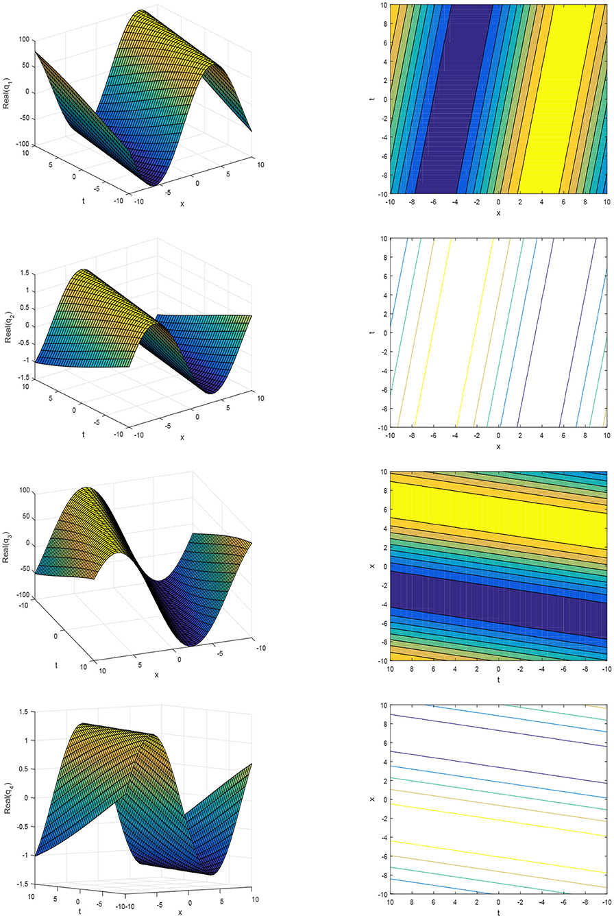
Figure 1. The 3D plots and contour plots of the real part of solution q₁(x, t) to q₄(x, t) for different parameters.

For case 2: The values of the parameters are

$\begin{array}{l}{a}_0=0,a_1=\sqrt{\frac{-2B{\alpha }_2}{{\alpha }_1({\alpha }_3+{\alpha }_5)}},b_1=0,B=-\frac{1}{2{\alpha }_2}({\alpha }_3+{\alpha }_5){\alpha }_1{a}_1^2\end{array}$

and the corresponding combined dark-singular wave structures are constructed.

For γ < 0, the following type of exact solutions of Equation (1.1) is written:

$\begin{array}{l}{q}_{j_6}=q_6=\sqrt{\frac{2rB{\alpha }_2}{{\alpha }_1({\alpha }_3+{\alpha }_5)}}tanh(i\sqrt{r}\xi )\times e^{i\varphi },\\ \end{array}$

The following two cases are obtained from the above solution and considered as the diagonal components of the spin ladder.

$\begin{array}{l}{q}_{6,1}=\left[\sqrt{\frac{2rB{\alpha }_2}{{\alpha }_1({\alpha }_3+{\alpha }_5)}}tanh(i\sqrt{r}B(x-\nu t))\right]\\ cos\left(-\left(\frac{{\alpha }_3+{\alpha }_5}{{\alpha }_2}\right)x+wt+\theta \right)\\ q_{6,1}=\left[\sqrt{\frac{2rB{\alpha }_2}{{\alpha }_1({\alpha }_3+{\alpha }_5)}}tanh(i\sqrt{r}B(x-\nu t))\right]\\ sin\left(-\left(\frac{{\alpha }_3+{\alpha }_5}{{\alpha }_2}\right)x+wt+\theta \right)\\ \end{array}$

and we also have

$\begin{array}{l}{q}_{j_7}=q_7=\sqrt{\frac{2rB{\alpha }_2}{{\alpha }_1({\alpha }_3+{\alpha }_5)}}coth(i\sqrt{r}\xi )\times e^{i\varphi }.\end{array}$

For γ > 0, one may have the following periodic solutions

$\begin{array}{l}{q}_{j_8}=q_8=i\sqrt{\frac{2rB{\alpha }_2}{{\alpha }_1({\alpha }_3+{\alpha }_5)}}tan(\sqrt{r}\xi )\times e^{i\varphi },\end{array}$

and

$\begin{array}{l}{q}_{j_9}=q_9=-i\sqrt{\frac{2rB{\alpha }_2}{{\alpha }_1({\alpha }_3+{\alpha }_5)}}cot(\sqrt{r}\xi )\times e^{i\varphi }.\end{array}$

For γ = 0, one may have the following periodic solutions

$\begin{array}{l}{q}_{j_{10}}=q_{10}=-\frac{i}{\xi }\sqrt{\frac{2B{\alpha }_2}{{\alpha }_1({\alpha }_3+{\alpha }_5)}}\times e^{i\varphi },\end{array}$

where,

$\begin{array}{l}\xi =-\frac{1}{2{\alpha }_2}({\alpha }_3+{\alpha }_5){\alpha }_1{a}_1^2(x-vt).\\ \end{array}$

The pattern of the solutions for q₆ to q₉ are shown in Figure 2 for the values of parameters α₁ = 0.007, α₂ = 0.98, α₃ = 0.01, r = 0.76, B = 0.98, k = 0.98, ξ = 0.01, θ = 0.2, and b = 1.5.

FIGURE 2

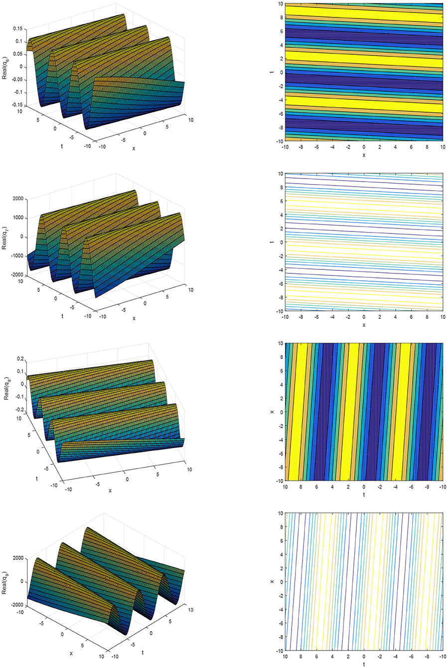
Figure 2. The 3D plots and contour plots of the real part of solution q₆(x, t) to q₉(x, t) for different parameters.

For case 3: The values of parameters are

$\begin{array}{l}{a}_0=b_1\sqrt{\frac{2}{r}},a_1=0,b_1=r\sqrt{\frac{-2B{\alpha }_2}{{\alpha }_1({\alpha }_3+{\alpha }_5)}},\\ B=-\frac{({\alpha }_3+{\alpha }_5){\alpha }_1{b}_1^2}{2r^2{\alpha }_2}\end{array}$

and the corresponding dark and singular wave structures can be obtained.

For γ < 0, the following forms of the exact solutions to Equation (1.1) are obtained.

$\begin{array}{l}{q}_{j_{11}}=q_{11}=[\sqrt{\frac{2b_1^2}{r}}-\sqrt{\frac{2rB{\alpha }_2}{{\alpha }_1({\alpha }_3+{\alpha }_5)}}coth(i\sqrt{r}\xi )]\times e^{i\varphi },\end{array}$

and

$\begin{array}{l}{q}_{j_{12}}=q_{12}=[\sqrt{\frac{2b_1^2}{r}}-\sqrt{\frac{2rB{\alpha }_2}{{\alpha }_1({\alpha }_3+{\alpha }_5)}}tanh(i\sqrt{r}\xi )]\times e^{i\varphi }.\end{array}$

The following two cases are obtained from the above solution and considered as the diagonal components of the spin ladder.

$\begin{array}{l}{q}_{12,1}=\left[\sqrt{\frac{2b_1^2}{r}}-\sqrt{\frac{2rB{\alpha }_2}{{\alpha }_1({\alpha }_3+{\alpha }_5)}}tanh(i\sqrt{r}B(x-\nu t))\right]\\ cos\left(-(\frac{{\alpha }_3+{\alpha }_5}{{\alpha }_2})x+wt+\theta \right)\\ q_{12,1}=\left[\sqrt{\frac{2b_1^2}{r}}-\sqrt{\frac{2rB{\alpha }_2}{{\alpha }_1({\alpha }_3+{\alpha }_5)}}tanh(i\sqrt{r}B(x-\nu t))\right]\\ sin\left(-(\frac{{\alpha }_3+{\alpha }_5}{{\alpha }_2})x+wt+\theta \right).\end{array}$

For γ > 0, one may have the following periodic solutions

$\begin{array}{l}{q}_{j_{13}}=q_{13}=\left[\sqrt{\frac{2b_1^2}{r}}+i\sqrt{\frac{2rB{\alpha }_2}{{\alpha }_1({\alpha }_3+{\alpha }_5)}}cot(\sqrt{r}\xi )\right]\times e^{i\varphi },\end{array}$

and

$\begin{array}{l}{q}_{j_{14}}=q_{14}=\left[\sqrt{\frac{2b_1^2}{r}}-i\sqrt{\frac{2rB{\alpha }_2}{{\alpha }_1({\alpha }_3+{\alpha }_5)}}tan(\sqrt{r}\xi )\right]\times e^{i\varphi },.\end{array}$

For γ = 0, one may have the following periodic solutions

$\begin{array}{l}{q}_{j_{15}}=q_{15}=\left[\sqrt{\frac{2b_1^2}{r}}-ir\xi \sqrt{\frac{2B{\alpha }_2}{{\alpha }_1({\alpha }_3+{\alpha }_5)}}\right]\times e^{i\varphi },\end{array}$

where,

$\begin{array}{l}\xi =-\frac{({\alpha }_3+{\alpha }_5){\alpha }_1{b}_1^2}{2r^2{\alpha }_2}(x-vt)\\ \varphi =\frac{2B{r}^2}{{\alpha }_1{b}_1^2}x+(\frac{5({\alpha }_3+{\alpha }_5){\alpha }_1{b}_1^2}{r{\alpha }_2}-{(\frac{{\alpha }_3+{\alpha }_5}{{\alpha }_2})}^2)t+\theta .\end{array}$

The pattern of the solutions for q₁₁ to q₁₄ are shown in Figure 3 for the values of parameters α₁ = 2, r = 1.5, B = 3.9, k = 0.98, ξ = 0.01, θ = 0.2, and b = 0.25.

FIGURE 3

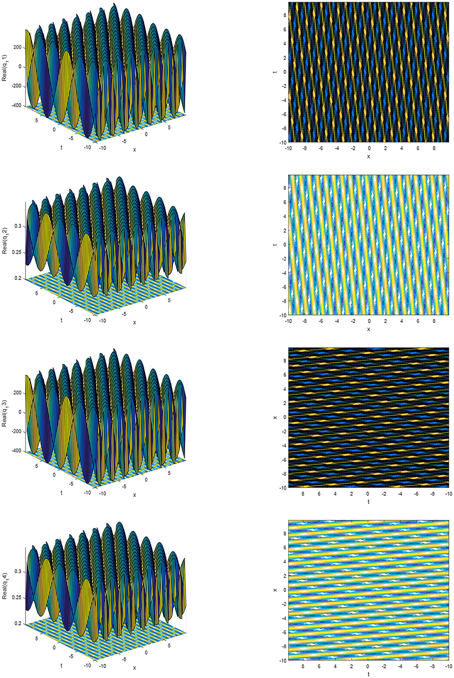
Figure 3. The 3D plots and contour plots of the real part of solution q₁₁(x, t) to q₁₄(x, t) for different parameters.

For case 4: The values of parameters are

$\begin{array}{l}{a}_0=0,a_1=0,b_1=r\sqrt{\frac{-2B{\alpha }_2}{{\alpha }_1({\alpha }_3+{\alpha }_5)}},B=-\frac{b_1^2({\alpha }_3+{\alpha }_5){\alpha }_1}{2{\alpha }_2{r}^2}\end{array}$

and the corresponding dark and singular wave structures can be obtained.

For γ < 0, the following exact solutions to Equation (1.1) are obtained.

$\begin{array}{l}{q}_{j_{16}}=q_{16}=-\sqrt{\frac{2rB{\alpha }_2}{{\alpha }_1({\alpha }_3+{\alpha }_5)}}coth(i\sqrt{r}\xi )\times e^{i\varphi }\end{array}$

and

$\begin{array}{l}{q}_{j_{17}}=q_{17}=-\sqrt{\frac{2rB{\alpha }_2}{{\alpha }_1({\alpha }_3+{\alpha }_5)}}tanh(i\sqrt{r}\xi )\times e^{i\varphi }.\end{array}$

The following two cases are obtained from the above solution and are considered the diagonal components of the spin ladder.

$\begin{array}{l}{q}_{17,1}=\left[-\sqrt{\frac{2rB{\alpha }_2}{{\alpha }_1({\alpha }_3+{\alpha }_5)}}tanh(i\sqrt{r}B(x-\nu t))\right]\\ cos\left(-(\frac{{\alpha }_3+{\alpha }_5}{{\alpha }_2})x+wt+\theta \right)\\ q_{17,1}=\left[-\sqrt{\frac{2rB{\alpha }_2}{{\alpha }_1({\alpha }_3+{\alpha }_5)}}tanh(i\sqrt{r}B(x-\nu t))\right]\\ sin\left(-(\frac{{\alpha }_3+{\alpha }_5}{{\alpha }_2})x+wt+\theta \right)\end{array}$

For γ > 0, one may have the following periodic solutions

$\begin{array}{l}{q}_{j_{18}}=q_{18}=i\sqrt{\frac{2rB{\alpha }_2}{{\alpha }_1({\alpha }_3+{\alpha }_5)}}cot(\sqrt{r}\xi )\times e^{i\varphi },\end{array}$

and

$\begin{array}{l}{q}_{j_{19}}=q_{19}=-i\sqrt{\frac{2rB{\alpha }_2}{{\alpha }_1({\alpha }_3+{\alpha }_5)}}tan(\sqrt{r}\xi )\times e^{i\varphi }.\end{array}$

For γ = 0, one may have the following periodic solutions

$\begin{array}{l}{q}_{j_{20}}=q_{20}=-ir\xi \sqrt{\frac{2B{\alpha }_2}{{\alpha }_1({\alpha }_3+{\alpha }_5)}}\times e^{i\varphi },\end{array}$

where

$\begin{array}{l}\xi =-\frac{b_1^2({\alpha }_3+{\alpha }_5){\alpha }_1}{2{\alpha }_2{r}^2}\left(x-vt\right).\end{array}$

The pattern of the solutions for q₁₆ to q₁₉ are shown in Figure 4 for the values of parameters α₁ = 0.002, r = 0.5, B = 0.9, k = 0.98, ξ = 0.01, θ = 0.2, and b = 0.25.

FIGURE 4

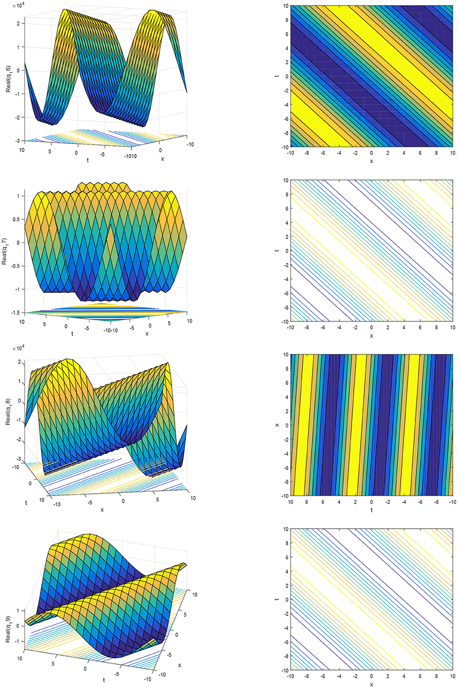
Figure 4. The 3D plots and contourplots of the real part of solution q₁₆(x, t) to q₁₉(x, t), for different parameters.

For case 5: The values of parameters are

$\begin{array}{l}{a}_0=0,b_1=r\sqrt{\frac{-2B{\alpha }_2}{{\alpha }_1({\alpha }_3+{\alpha }_5)}},\\ a_1=\frac{\omega {\alpha }_2^2+{({\alpha }_3+{\alpha }_5)}^2-2{\alpha }_2^{2}Br}{3b_1{\alpha }_1{\alpha }_2({\alpha }_3+{\alpha }_5)},\\ B=\frac{\omega {\alpha }_2^2+{({\alpha }_3+{\alpha }_5)}^2-3a_1{b}_1{\alpha }_1{\alpha }_2({\alpha }_3+{\alpha }_5)}{2r{\alpha }_2^2}\end{array}$

and the corresponding dark and singular wave structures are obtained.

For γ < 0, one can obtain the following exact solutions to Equation (1.1).

$\begin{array}{l}{q}_{j_{21}}=q_{21}=[-\frac{\omega {\alpha }_2^2+{({\alpha }_3+{\alpha }_5)}^2-2{\alpha }_2^{2}Br}{3b_1{\alpha }_1{\alpha }_2({\alpha }_3+{\alpha }_5)}i\sqrt{r}tanh(i\sqrt{r}\xi )\\ -\sqrt{\frac{2Br{\alpha }_2}{{\alpha }_1({\alpha }_3+{\alpha }_5)}}coth(i\sqrt{r}\xi )]\times e^{i\varphi }.\end{array}$

The following two cases are obtained from the above solution and considered as the diagonal components of the spin ladder.

$\begin{array}{l}{q}_{21,1}=[-\frac{\omega {\alpha }_2^2+{({\alpha }_3+{\alpha }_5)}^2-2{\alpha }_2^{2}Br}{3b_1{\alpha }_1{\alpha }_2({\alpha }_3+{\alpha }_5)}i\sqrt{r}tanh(i\sqrt{r}B(x-\nu t)\\ -\sqrt{\frac{2rB{\alpha }_2}{{\alpha }_1({\alpha }_3+{\alpha }_5)}}coth(i\sqrt{r}B(x-\nu t))]cos(-(\frac{{\alpha }_3+{\alpha }_5}{{\alpha }_2})x\\ +wt+\theta )\\ q_{21,1}=[-\frac{\omega {\alpha }_2^2+{({\alpha }_3+{\alpha }_5)}^2-2{\alpha }_2^{2}Br}{3b_1{\alpha }_1{\alpha }_2({\alpha }_3+{\alpha }_5)}i\sqrt{r}tanh(i\sqrt{r}B(x-\nu t)\\ -\sqrt{\frac{2rB{\alpha }_2}{{\alpha }_1({\alpha }_3+{\alpha }_5)}}coth(i\sqrt{r}B(x-\nu t))]sin(-(\frac{{\alpha }_3+{\alpha }_5}{{\alpha }_2})x\\ +wt+\theta ),\end{array}$

and

$\begin{array}{l}{q}_{j_{22}}=q_{22}=[-\frac{\omega {\alpha }_2^2+{({\alpha }_3+{\alpha }_5)}^2-2{\alpha }_2^{2}Br}{3b_1{\alpha }_1{\alpha }_2({\alpha }_3+{\alpha }_5)}i\sqrt{r}coth(i\sqrt{r}\xi )\\ -\sqrt{\frac{2Br{\alpha }_2}{{\alpha }_1({\alpha }_3+{\alpha }_5)}}tanh(i\sqrt{r}\xi )]\times e^{i\varphi }.\end{array}$

For γ > 0, one may have the following periodic solutions

$\begin{array}{l}{q}_{j_{23}}=q_{23}=[\frac{\omega {\alpha }_2^2+{({\alpha }_3+{\alpha }_5)}^2-2{\alpha }_2^{2}Br}{3b_1{\alpha }_1{\alpha }_2({\alpha }_3+{\alpha }_5)}\sqrt{r}tan(\sqrt{r}\xi )\\ +\sqrt{\frac{-2Br{\alpha }_2}{{\alpha }_1({\alpha }_3+{\alpha }_5)}}cot(\sqrt{r}\xi )]\times e^{i\varphi }\\ q_{j_{24}}=q_{24}=[-\frac{\omega {\alpha }_2^2+{({\alpha }_3+{\alpha }_5)}^2-2{\alpha }_2^{2}Br}{3b_1{\alpha }_1{\alpha }_2({\alpha }_3+{\alpha }_5)}\sqrt{r}cot(\sqrt{r}\xi )\\ -\sqrt{\frac{-2Br{\alpha }_2}{{\alpha }_1({\alpha }_3+{\alpha }_5)}}tan(\sqrt{r}\xi )]\times e^{i\varphi }\end{array}$

For γ = 0, one may have the following periodic solutions

$\begin{array}{l}{q}_{j_{25}}=q_{25}=[-\frac{\omega {\alpha }_2^2+{({\alpha }_3+{\alpha }_5)}^2-2{\alpha }_2^{2}Br}{3b_1{\alpha }_1{\alpha }_2({\alpha }_3+{\alpha }_5)}(\frac{1}{\xi })\\ -r\xi \sqrt{\frac{-2B{\alpha }_2}{{\alpha }_1({\alpha }_3+{\alpha }_5)}}]\times e^{i\varphi }\end{array}$

where

$\begin{array}{l}\xi =\frac{\omega {\alpha }_2^2+{({\alpha }_3+{\alpha }_5)}^2-3a_1{b}_1{\alpha }_1{\alpha }_2({\alpha }_3+{\alpha }_5)}{2r{\alpha }_2^2}\left(x-vt\right).\end{array}$

These are the new solitons and periodic wave structures.

4. Conclusions

The article gives single and combined electromagnetic wave structures for the coupled non-linear Schrödinger equations along with the coefficients of ferromagnetic spin exchange interaction, antiferromagnetic coupling, exchange coupling, and single-ion uniaxial anisotropy. The model under investigation describes the dynamic behavior of electromagnetic waves in a spin ladder antiferromagnetic medium. First the complex transformation is used and then modified extended direct algebraic method is utilized to find dark, singular, and dark-singular wave structures. Some other solutions (singular periodic) are also fall out during the analytical analysis. The constraint conditions for the existence of wave structures for different parameters are also observed. Moreover, the 3D plots and corresponding contour plots of the real part of solutions are drawn by choosing suitable parameters.

It is also observed that the method used is effective, powerful, reliable, and much more practical in obtaining the exact wave structures for non-linear phenomena that arise in fields like telecommunication engineering, mathematical biology, mathematical physics, an ocean engineering and vice versa.

Data Availability Statement

The original contributions presented in the study are included in the article/supplementary materials, further inquiries can be directed to the corresponding author/s.

Author Contributions

MY, SR, and DB contributed to conception and design of the study. MY and UY performed the analytical analysis. NA and MI established the results. NA and UY draw the graphs using mathematical. MI and UY wrote the first draft of manuscript. MY, SR, NA, and DB wrote sections of the manuscript. All authors contributed to manuscript revision, read, and approved the submitted version.

Conflict of Interest

The authors declare that the research was conducted in the absence of any commercial or financial relationships that could be construed as a potential conflict of interest.

References

1. Esbensen BK, Bache M, Bang O, Krolikowski W. Anomalous interaction of nonlocal solitons in media with competing nonlinearities. Phys Rev A. (2012) 86:033838. doi: 10.1103/PhysRevA.86.033838

CrossRef Full Text | Google Scholar

2. Chen W, Shen M, Kong Q, Shi J, Wang Q, Krolikowski W. Interactions of nonlocal dark solitons under competing cubic-quintic nonlinearities. Opt Lett. (2014) 39:1764. doi: 10.1364/OL.39.001764

PubMed Abstract | CrossRef Full Text | Google Scholar

3. Krolikowski W, Bang O, Nikolov NI, Neshev D, Wyller J, Rasmussen JJ, et al. Modulational instability solitons and beam propagation in spatially nonlocal nonlinear media. J Opt B Quantum Semiclass Opt. (2004) 6:288. doi: 10.1088/1464-4266/6/5/017

PubMed Abstract | CrossRef Full Text | Google Scholar

4. Krolikowski W, Bang O, Rasmussen JJ, Wyller J. Modulational instability in nonlocal nonlinear Kerr media. Phys Rev E. (2001) 64:016612. doi: 10.1103/PhysRevE.64.016612

PubMed Abstract | CrossRef Full Text | Google Scholar

5. Wyller J, Krolikowski W, Bang O, Rasmussen JJ. Generic features of modulational instability in nonlocal Kerr media. Phys Rev E. (2002) 66:066615. doi: 10.1103/PhysRevE.66.066615

PubMed Abstract | CrossRef Full Text | Google Scholar

6. Bang O, Krolikowski W, Wyller J, Rasmussen JJ. Collapse arrest and soliton stabilization in nonlocal nonlinear media. Phys Rev E. (2002) 66:046619. doi: 10.1103/PhysRevE.66.046619

PubMed Abstract | CrossRef Full Text | Google Scholar

7. Kartashov YV, Vysloukh VA, Torner L. Tunable soliton self-bending in optical lattices with nonlocal nonlinearity. Phys Rev Lett. (2004) 93:153903. doi: 10.1103/PhysRevLett.93.153903

PubMed Abstract | CrossRef Full Text | Google Scholar

8. Xu Z, Kartashov YV, Torner L. Soliton mobility in nonlocal optical lattices. Phys Rev Lett. (2005) 95:113901. doi: 10.1103/PhysRevLett.95.113901

PubMed Abstract | CrossRef Full Text | Google Scholar

9. Rotschild C, Cohen O, Manela O, Segev M, Carmon T. Solitons in nonlinear media with an infinite range of nonlocality: first observation of coherent elliptic solitons and of vortex-ring solitons. Phys Rev Lett. (2005) 95:213904. doi: 10.1103/PhysRevLett.95.213904

PubMed Abstract | CrossRef Full Text | Google Scholar

10. Islam W, Younis M. Weakly nonlocal single and combined solitons in nonlinear optics with cubic quintic nonlinearities. J Nano Optoelectron. (2017) 12:1008–12. doi: 10.1166/jno.2017.2096

CrossRef Full Text | Google Scholar

11. Younis M, Bilal M, Rehman S, Younas U, Rizvi STR. Investigation of optical solitons in birefringent polarization preserving fibers with four-wave mixing effect. Int J Mod Phys B. (2020) 34:2050113. doi: 10.1142/S0217979220501131

CrossRef Full Text | Google Scholar

12. Ali S, Younis M. Rogue wave solutions and modulation instability with variable coefficient and harmonic potential. Front Phys. (2020) 7:255. doi: 10.3389/fphy.2019.00255

CrossRef Full Text | Google Scholar

13. Younas B, Younis M. Chirped solitons in optical monomode fibres modelled with Chen-Lee-Liu equation. Pramana J Phys. (2020) 94:3. doi: 10.1007/s12043-019-1872-6

CrossRef Full Text | Google Scholar

14. Chen SJ, Yin YH, Ma WX, Lu X. Abundant exact solutions and interaction phenomena of the (2 + 1)-dimensional YTSF equation. Anal Math Phys. (2019) 9:2329–44. doi: 10.1007/s13324-019-00338-2

CrossRef Full Text | Google Scholar

15. Chen SJ, Ma WX, Lu X. Backlund transformation, exact solutions and interaction behaviour of the (3+1)-dimensional Hirota-Satsuma-Ito-like equation. Commun Nonlin Sci. (2020) 83:105135. doi: 10.1016/j.cnsns.2019.105135

CrossRef Full Text | Google Scholar

16. Xu HN, Ruan WY, Zhang Y, Lu X. Multi-exponential wave solutions to two extended Jimbo-Miwa equations and the resonance behavior. Appl Math Lett. (2020) 99:105976. doi: 10.1016/j.aml.2019.07.007

CrossRef Full Text | Google Scholar

17. Usman MS, Baleanu D, Tariq KUH, Kaplan M, Younis M, Rizvi STR. Different types of progressive wave solutions via the 2D-chiral nonlinear Schrödinger equation. Front Phys. (2020) 8:215. doi: 10.3389/fphy.2020.00215

CrossRef Full Text | Google Scholar

18. Osman MS, Tariq KU, Bekir A, Elmoasry A, Elazab NS, Younis M, et al. Investigation of soliton solutions with different wave structures to the (2 + 1)-dimensional Heisenberg ferromagnetic spin chain equation. Commun Theor Phys. (2020) 72:035002. doi: 10.1088/1572-9494/ab6181

CrossRef Full Text | Google Scholar

19. Shen M, Lin YY, Jeng CC, Lee RK. Vortex pairs in nonlocal nonlinear media. J Opt. (2012) 14:065204. doi: 10.1088/2040-8978/14/6/065204

CrossRef Full Text | Google Scholar

20. Buccoliero D, Desyatnikov AS, Krolikowski W, Kivshar YS. Laguerre and Hermite soliton clusters in nonlocal nonlinear media. Phys Rev Lett. (2007) 98:053901. doi: 10.1103/PhysRevLett.98.053901

PubMed Abstract | CrossRef Full Text | Google Scholar

21. Alfassi B, Rotschild C, Manela O, Segev M, Christodoulides DN. Nonlocal surface-wave solitons. Phys Rev Lett. (2007) 98:213901. doi: 10.1103/PhysRevLett.98.213901

PubMed Abstract | CrossRef Full Text | Google Scholar

22. Shen M, Wang Q, Shi J, Chen Y, Wang X. Nonlocal incoherent white-light solitons in logarithmically nonlinear media. Phys Rev E. (2005) 72:026604. doi: 10.1103/PhysRevE.72.026604

PubMed Abstract | CrossRef Full Text | Google Scholar

23. Rotschild C, Schwartz T, Cohen O, Segev M. Incoherent solitons in effectively instantaneous nonlocal nonlinear media. Nat Photonics. (2008) 2:371. doi: 10.1038/nphoton.2008.81

CrossRef Full Text | Google Scholar

24. Shen M, Ding H, Kong Q, Ruan L, Pang S, Shi J, et al. Self-trapping of two-dimensional vector dipole soliton in nonlocal media. Phys Rev A. (2010) 82:043815. doi: 10.1103/PhysRevA.82.043815

CrossRef Full Text | Google Scholar

25. Alberucci A, Peccianti M, Assanto G, Dyadyusha A, Kaczmarek M. Two-color vector solitons in nonlocal media. Phys Rev Lett. (2006) 97:153903. doi: 10.1103/PhysRevLett.97.153903

PubMed Abstract | CrossRef Full Text | Google Scholar

26. Kavitha L, Parasuraman E, Gopi D, Bhuvaneswari S. Propagation of electromagnetic solitons in an antiferromagnetic spinladder medium. J Electromagnet Wave. (2016) 30:740–66. doi: 10.1080/09205071.2015.1137500

CrossRef Full Text | Google Scholar

27. Younis M, Rehman HU, Iftikhar M. Travelling wave solutions to some nonlinear evolution equations. Appl Math Comput. (2014) 249:81–8. doi: 10.1016/j.amc.2014.09.104

PubMed Abstract | CrossRef Full Text | Google Scholar